A Design Method of Reference Model for near Time Optimal Model-Following Servo Controller: A Case Study for Multi-Zone Heating System with Input Saturation

(1)

A Design Method of Reference Model for near Time

Optimal Model-Following Servo Controller: A Case

Study for Multi-Zone Heating System with Input

Saturation

Kazuhiro Mimura1_{, Tetsuo Shiotsuki}2,*

1_{System R&D Department, KELK Ltd., Kanagawa, Japan}

2_{Department of Robotics and Mechatronics, Tokyo Denki University, Tokyo, Japan}

Abstract

This paper proposes a design method of reference model for model-following servo (MFS) control which overcomes the difficulty of control input saturation. One typical application of MFS control is heating and/or cooling plate control of semiconductor wafer fabrication. The control object is inherently MIMO (Multi Input Multi Output) system with interaction and input saturation and requires both temperature uniformity and faster response. MFS control is a well-known effective technique for tracking control of MIMO system with interaction and disturbances. However input saturation obstacles the accomplishment of the control requirements In order to overcome this difficulty we introduce a new design method of reference model and input signal based on master-slave step response tests and near time optimal simulations. Experimental results indicate the effectiveness of the proposed reference model design method which realizes both faster response and better uniformity.

Keywords

Reference Model, Model-Following Servo Control, Optimal Control, Time Optimal Control

1. Introduction

Many of the industrial processes are MIMO system with interaction. One typical application is heating and/or cooling plate for semiconductor wafer fabrication. The plate usually consists of multiple zones and each zone temperature should be controlled accurately. The requirements to the temperature control are

(1) The temperature should reach the set-point variable (SV) as quick as possible to realize high throughput. (2) Temperature uniformity or temperature gradient is kept constant both transient and steady state response.

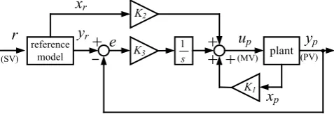
In spite of these requirements, temperature control is very challenging due to the interactions between the neighbour zones and many studies have been conducted [1-3]. Model-following servo (MFS) control [4, 5] is suitable for the MIMO system with interaction because, 1) it has the advantage of the optimal control such as stability and robustness, 2) we need not consider decoupling design explicitly. As shown in Figure 1, the MFS control consists

* Corresponding author:

[email protected] (Tetsuo Shiotsuki) Published online at http://journal.sapub.org/control

of plant, reference model, integrator, state feedback gain K1 from the plant, feedforward gain K2 from the reference model, and gain K3 for the integrator. A low order system that has a desired dynamics is usually chosen as a reference model. The process variable, yp, follows the step response of the reference model, yr.

Figure 1. The structure of the model following servo control

For the multi-zone heating system, if we use same reference model, all process variables (PV) follow the same reference trajectory, which realizes the above requirement (2). Control systems in real world however usually contain constraint such as actuator saturation. Applying MFS control to such system worsens its control performance. We have to find low order system as a reference model that satisfies desired response speed without saturating manipulated variable (MV). However, in order to satisfy the above requirement (1) the MV should be maximum

reference

model s plant

1

K1

K2

K3

+

- ++ +

xr

xp

yp

up

r yr _e

(2)

(saturated). As a result, some of the PVs can not follow reference trajectory and temperature uniformity worsens. Although the MFS control has been studied for long time [6-12], no studies show the negative effect of saturation on MFS control for MIMO system. Other than the MFS control, reference governor [13, 15] and model predictive control [16, 17] are able to consider constraint explicitly. The reference governor reshapes the reference signal so that its state and/or MV always stay within the constraints. It is very effective method since we can design reference governor and feedback controller independently. However this method only guarantees constraint fulfilment but not response speed specification. In order to guarantee both constraint fulfilment and response speed, two different optimization problems must be solved iteratively [14]. Model predictive control is a powerful control method that can easily handle dead-time system, non-minimum phase system, and system with constraints. However it requires several parameter tunings such as the number of the step of the each horizon and weight for the cost functions.

In this paper we propose a simple yet practical design method of reference model for the MFS control. It is suitable for the MIMO system with interaction and input saturation. The method provides ideal reference model that enables near time optimal response and uniformity of PVs. This paper consists of five sections. In section 2, we explain disadvantage of conventional MFS control by showing some experimental results. In section 3, proposed design method is explained. In section 4, the effectiveness of our proposed method is shown by an experimental result. And section 5 concludes this study.

2. Disadvantage of Conventional MFS

Control

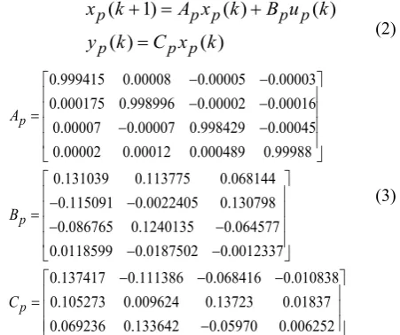
Figure 2 illustrates test plant for the temperature control of an aluminium plate which size is 400 x 150 x t4. Three Peltier modules for heating and cooling are allocated unsymmetrically in a longitudinal direction of the plate. Plate temperatures are measured by three Type-K thermocouples. Each of them is allocated near the Peltier module. Zone number is assigned as zone 1, 2, and 3 from the left.

We designed conventional MFS controller for this test plant. In order to obtain a plant model we conducted step response experiment for one zone at a time. Each response data is approximated by a first order plus dead time model. Whole test plant model is expressed by transfer function matrix as shown in eq. (1).

2 9 110

31 2 47

100 42 2

38.6 18.4 6.3

102 1 192 1 318 1

17.0 29.2 11.7

( )

214 1 101 1 239 1

8.9 12.9 31.4

321 1 244 1 119 1

s s s

p

s s s

e e e

s s s

G s e e e

s s s

e e e

s s s

− − − − − − − − −    ₊ ₊ ₊      =  ₊ ₊ ₊       + + +    (1)

Replacing dead time to a first order Pade approximation, eq. (1) is converted to a discrete time state space model with its sampling time 0.1 sec. At the same time balanced realization and reduced order realization are applied to the model.

By these realizations, the model originally eighteenth order is reduced to the fourth order as shown eq. (2) where its coefficient Ap, Bp, and Cpare (3).

( 1) ( ) ( )

( ) ( )

p p p p p

p p p

x k A x k B u k

y k C x k

+ = +

= (2)

0.999415 0.00008 0.00005 0.00003 0.000175 0.998996 0.00002 0.00016 0.00007 0.00007 0.998429 0.00045 0.00002 0.00012 0.000489 0.99988 0.131039 0.113775 0.068144

0.115091 0.0022405 0.130798 0.08676 p p A B − −    ₋ ₋    =  − −      − − =

− 5 0.1240135 0.064577 0.0118599 0.0187502 0.0012337 0.137417 0.111386 0.068416 0.010838 0.105273 0.009624 0.13723 0.01837 0.069236 0.133642 0.05970 0.006252

p C        −   ₋ ₋    − − −     =    −    (3)

We chose second order plus dead time system as a reference model. It’s undamped natural frequency, ω0 is 1/45 red/sec, damping ratio, ζ is 0.9, and dead time is 2 sec. The MV does not saturate in its response. Applying this to all zone, the reference model, Gr(s), is

( ) 0 0

( ) ( ) ( ) 0 ( ) 0 ( )

0 0 ( )

r

r r r

r

g s

y s G s r s g s r s g s     = _{= } _     (4) where 2

2 2 1

( ) .

(45) 2 0.9 45 1

s r

g s e

s s

− =

+ ⋅ ⋅ + (5)

Replacing dead time to a first order Pade approximation, eq. (4) is converted to a discrete time state space model (6) with its sampling time 0.1 sec.

( 1) ( ) ( )

( ) ( )

r r r r

r r r

x k A x k B r k y k C x k

+ = +

= (6)

where

0 0 0.90103 0.01539 0.00600

0 0 0.02374 0.99980 0.00007

0 0 0.00003 0.00312 0.99999

0 0 0.02374

0 0 0.00030

0 0 0.0000003

0 0

0 0 0 0.007

0 0

r

r r r

r r

r r r

r r

r r r

r

a

A a a

a b

B b b

b c

C c c

c − −         =_ _ =_ − _                 =_ _ =_ _             =_ _ = −    

[

90 0.25283 .

]

(3)

Top: illustrated system setup. Bottom: Picture of actual system

Figure 2. Test plant for the temperature control of aluminium plate

With eq. (2) and eq. (6), an augmented system is derived from appendix.

( 1) ( ) ( )

( ) ( )

a a a a p

a a

X k A X k B u k e k C X k

+ = + ∆

= (8)

The optimal control law minimizing the performance index (9)

2 2

1

( )_Q p( )_R

k

J e k u k

∞

=

 

= _ + ∆ _

 

∑

(9)

is given by

1 2 3

1

( ) ( ) ( ) ( )

k

p p r

j

u k K x k K x k K e j

=

= + +

∑

(10)

where we set weight matrices Q, R as

13 13 13 3 3 13 3 3

50000 0 0

0 0

, 0 100000 0 .

0

0 0 50000

Q R

I

× ×

 

  _ _

=_ _ =_ _

  _ _

 

(11)

Gain K1, K2, and K3 are calculated as

1

2

0.05805 0.05114 0.03939 0.00481 0.04814 0.00435 0.05664 0.00616 0.04038 0.07225 0.03224 0.00364 0.00816 0.0399 0.11391 0.00216 0.00045 0.00184 0.00048 0.0107 0.00034 0.0015 0.00249 0.00008 0.

K

− − −

 

 

=  

 − 

 

− − −

 

=_ − −

− − −



3

00974 0.01914 0.00026 0.00118 0.00175 0.04995 0.13114 0.00009 0.00040 0.00090 0.00037 0.00076 0.01163 0.05529 0.16405

0.00442 0.00027 0.00001 0.00019 0.00313 0.00001 0.00001 0.00002 0.00443

K

− − − 



− − − − − _



− − − _

− −

 

 

=  

 − 

 

(12)

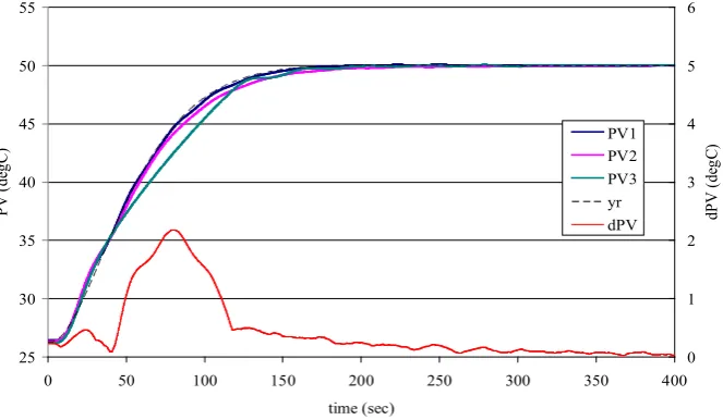
We added integrator anti-windup and state estimator for the feedback gain K1. Figures 3 show result of set-point response experiment. Figure 3(a) shows zone temperature (PV1, PV2, and PV3), reference trajectory yr, and temperature uniformity, dPV defined by eq. (13).

max min 1,2,3

dPV = PVi− PVi i= (13) figure 3(b) shows the MV of each zone. As the figures indicate, all zone temperatures follow reference trajectory quite close and temperature uniformity is less than 0.35 deg C. All MVs do not saturate as we designed.

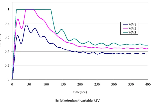
In order to speed up the response, we changed undamped natural frequency of the reference model from 1/45 rad/sec to 1/30 rad/sec. The experimental result is shown in Figure 4. Graph legends are the same as figure 3. The response speed of the PVs becomes faster while the MV of zone 3 saturates. However, the PV of zone 3 cannot follow reference trajectory because the saturation limits its maximum speed. As a result the temperature uniformity during the transient response worsens by 2.1 deg C. From these experimental results it is clear that the conventional MFS control cannot maintain uniformity when its MV saturates. Conventional MFS control uses low order system as a reference model whose step response satisfies desired response specification. Therefore its response speed is the same as the step response of the reference model but not its maximum speed.

Controller

Power Supply

Heat Sink Cooloing Fan Aluminum Plate

Peltier Module K-Type Thermocouple zone 1 zone 2 zone 3

60 160

350 400 80

190 320

15

0

K-Type Thermocouple

Peltier Module

Aluminum Plate t4 zone 1 zone 2

(4)

(a) PV, reference trajectory yr, uniformity dPV

(b) Manipulated variable MV

Figure 3. Experimental result of set-point response. Reference model parameter ω0=1/45 rad/sec, ζ=0.9

25 30 35 40 45 50 55

0 50 100 150 200 250 300 350 400

time (sec)

PV

(d

eg

C)

0 1 2 3 4 5 6

dP

V

(de

gC

)

PV1 PV2 PV3 yr dPV

0 0.2 0.4 0.6 0.8 1

0 50 100 150 200 250 300 350 400 time(sec)

M

V

(0

-1

)

MV1 MV2 MV3

25 30 35 40 45 50 55

0 50 100 150 200 250 300 350 400

time (sec)

PV

(d

eg

C)

0 1 2 3 4 5 6

dP

V

(de

gC

)

(5)

Figure 4. Experimental result of set-point response. Reference model parameter ω0=1/30 rad/sec, ζ=0.9

3. Proposed Design Method

Figure 5 shows a staircase MV pattern that achieves time optimal response. The MV should be maximum until PV reaches to a point X. After passing the point X the MV should be changed to minimum to decelerate the speed. When the PV reaches to the SV, the MV is switched to a steady state value, MVss that can keep PV at SV. There are two ways to observe switching point, one is to watch PV and switch MV at the optimal point X, another is to time and switch MV at the optimal time t1and t2.

Figure 5. Ideal manipulate variable pattern for the time optimal control

We employ this idea to design reference model as illustrated in Figure 6. Unlike the conventional method shown in Figure 6(a), proposed method in Figure 6(b) first converts SV into corresponding MV pattern that satisfies time optimal response. The optimal MV pattern is then applied to the plant model to produce reference trajectory.

Although this idea is suitable for the SISO (single input single output) system it has a difficulty for the MIMO system. For the MIMO system, we have to design MV patterns for all inputs. However the interaction of the plant model makes design MV pattern difficult.

(a) Conventional method

(b) Proposed method

Figure 6. Comparison of the reference model

To cope with this difficulty, we simplified the plant model from an experimental result and designed MV pattern by simulation. The design procedure is explained below.

1) Master-Slave step response experiment

In order to find fastest response that can maintain uniformity of PVs, one of the zones which has the slowest response speed is chosen and assigned as a master zone. Maximum MV is applied to the master zone and the rest of the zones are made follow the master zone. This experiment can be realized by master-slave PID control.

0 0.2 0.4 0.6 0.8 1

0 50 100 150 200 250 300 350 400

time(sec)

M

V

(0

-1

)

MV1 MV2 MV3

SV

MV t

t 100%

0%

MVss

t1

t2 X

reference model

SV

t t

SV

yr

SV

plant model

yr

MV MV

pattern MV

t

SV

t SV

(6)

Figure 7. Experimental result for the master-slave response

2) System identification

A first order plus dead time model, Gm(s) can be build from the response data of the master zone. Dead time is replaced to a first order Pade approximation.

3) Seeking staircase MV pattern

The staircase MV pattern that realizes time optimal response of the Gm(s) is sought by iterative simulation. Here we set t2=t1 to shorten the simulation time. Although the response obtained becomes near time optimal the rising time up to 99% is almost the same as the time optimal case. We evaluate optimal MV pattern by overshoot of PV and IAE (Integral Absolute Error) criteria expressed eq. (14).

0

( ) T ( ) ( )

J t =

∫

SVτ −PV τ dt (14)

4) Building a reference model

The reference model Gr(s) is obtained by assigning Gm(s) to all zones. With this method, all reference trajectories are the same, which guarantees PV’s uniformity.

4. Experiment for Validation

In order to validate the effectiveness, the proposed method was applied to the test plant controller and the same experiment shown in section 2 was conducted.

1) Master-Slave step response experiment

Zone 3 was the slowest zone and assigned as master zone. Under the master-slave PID control configuration, maximum MV was set to the master zone and made rest of the zones follow. Figure 7 shows the result. Since MV3 for the master zone is maximum, this response is the fastest that can maintain uniformity of PVs. The uniformity after 50 seconds form the beginning is less than 0.1 deg C.

2) System Identification

A first order plus dead time model was identified as (15). 4

44.2 ( )

178 1 s

m

G s e

s

− =

+ (15) Replacing dead time to a first order Pade approximation, we obtained (16).

44.2 0.5

( )

178 1 0.5

m s

G s

s s

− +

= ⋅

+ + (16)

(a) MV pattern

(b) Reference trajectory

Figure 8. MV pattern and reference trajectory

20 30 40 50 60 70 80

0 100 200 300 400 500 600 700 800 time(sec)

PV

(d

eg

C

)

0 0.2 0.4 0.6 0.8 1 1.2

M

V

, d

PV

(d

egC

)

PV1 PV2 PV3 MV1 MV2 MV3 dPV

0 0.2 0.4 0.6 0.8 1

0 100 200 300 400 time (sec)

M

V

(0

-1

)

148

0 5 10 15 20 25 30

0 100 200 300 400

time (sec)

yr (d

eg

(7)

3) Seeking staircase MV pattern

Iterative simulation to seek the optimal switching time, t1 was executed by using Gm(s). Temperature width form the equilibrium to the SV was 25 deg C. The t1 was incremented 0.1 sec in each iteration. The optimal switching time obtained was 148 sec and the MV at steady state was MVss=25/44.2=0.56. Figure 8(a) shows MV pattern obtained and figure 8(b) shows reference model output. 4) Building a reference model

Assigning eq. (16) to all zones, the reference model was obtained. Discrete time state space model is the same equation as eq. (6) where

0 0

1.9507 0.9507

0 0

1 0

0 0

r

r r r

r

a

A a a

a

 

−

 

 

=_ _ _{= } _

 

 

 

[

]

0 0

0.25

0 0

0

0 0

0 0 0.0944 0.0993 .

0 0

r

r r r

r r

r r r

r

b

B b b

b c

C c c

c

 

 

=_ _ _{= } _

 

 

 

 

 

=_ _ = −

 

 

(17)

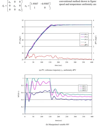
Using this reference model and MV pattern we conducted set-point response experiment which was the same as the one shown in section 2. The SV was 51.5 deg C, 25 deg C above the equilibrium temperature. Figure 9 show the result. Graph legends are the same as figure 3. Compare to the conventional method shown in figure 3 and 4, both response speed and temperature uniformity are improved.

Figure 9. Experimental result of proposed method

25 30 35 40 45 50 55

0 50 100 150 200 250 300 350 400

time (sec)

PV

(d

eg

C)

0 1 2 3 4 5 6

dP

V

(de

gC

)

PV1 PV2 PV3 yr dPV

0 0.2 0.4 0.6 0.8 1

0 50 100 150 200 250 300 350 400

time(sec)

M

V

(0

-1

)

(8)

5. Conclusions

We proposed a simple yet practical design method of reference model for the MFS control. It is suitable for the MIMO system with interaction and input saturation. In this paper we first claimed disadvantages of conventional method by showing experimental result. It indicates input saturation worsens both uniformity of PVs and response speed. In our proposed method we introduced unique reference model design and input signal design. The reference model is obtained by master-slave step response test. Using this model, staircase input signal that realizes near time optimal response is obtained by simulation. We showed the effectiveness of our method by experimental result. The result showed improvement of both response speed and temperature uniformity compare to the conventional method. Future work is to create method applicable to both heating and cooling that have different dynamics.

Appendix

Discrete time MFS control

Consider an m-inputs m-outputs plant

( 1) ( ) ( )

( ) ( )

p p p p p

p p p

x k A x k B u k y k C x k

+ = +

= (A1a)(A1b)

where n n

p R

A ∈ × , n m

p R

B ∈ × , m n

p R

C ∈ × , and xp, up, yp are states, manipulated variable, and process variable respectively. We assume (Ap, Bp) is controllable, and (Cp, Ap) is observable. A reference model is expressed

m-inputs and m-outputs system shown eq. (A2).

( 1) ( ) ( )

( ) ( )

r r r r

r r r

x k A x k B r k y k C x k

+ = +

= (A2a)(A2b)

where l l

r R

A ∈ × , l m

r R

B ∈ × , ml

r R

C ∈ × , and xr, r, yr are states, reference, and reference output respectively. We assume (Ar, Br) is controllable, (Cr, Ar) is observable, and the model is asymptotically stable. Considering difference equation of eq. (A1a) and (A2a), we obtain

{

} {

}

( 1) ( 1) ( )

( ) ( ) ( 1) ( 1)

( ) ( )

p p p

p p p p p p p p

p p p p

x k x k x k

A x k B u k A x k B u k A x k B u k

∆ + = + − = + − − + − = ∆ + ∆ (A3) and

{

} {

}

( 1) ( 1) ( )

( ) ( ) ( 1) ( 1)

( ) ( ) .

r r r

r r r r r r

r r r

x k x k x k

A x k B r k A x k B r k A x k B r k

∆ + = + −

= + − − + −

= ∆ + ∆

(A4)

An error signal is defined as (A5).

( ) _r( ) _p( )

e k =y k −y k (A5) Using equations from (A1) to (A5), first order difference

equation of the error signal is

( 1) ( 1) ( )

[ ( 1) ( 1)] [ ( ) ( )]

[ ( 1) ( 1)]

[ ( ) ( )]

( 1) ( 1)

[ ( ) ( )]

[ ( ) ( )].

r p r p

r r p p

r r p p

r r r r r

p p p p p

e k e k e k

y k y k y k y k C x k C x k

C x k C x k C x k C x k C A x k B u k

C A x k B u k

∆ + = + − = + − + − − = + − + − − = ∆ + − ∆ + = ∆ + ∆ − ∆ + ∆ (A6)

From Eq. (A3), (A4), and (A6), and assuming Δr(k)=0,

the following augmented system is obtained.

( 1) ( ) ( )

( ) ( )

a a a a p

a a

X k A X k B u k e k C X k

+ = + ∆

= (A7a)(A7b)

Where

[

]

( ) 0 0

( ) , 0 0

( )

0 , 0 0 .

p p

a r a r

p p r r

p

a a

p p

x k A

X x k A A

e k C A C A I

B

B C I

C B ∆         = ∆_ _ =_ _   ₋          =_ _ = ₋   

The optimal control law minimizing the performance index (A8)

2 2

1

( )_Q _p( )_R k

J e k u k

∞

=

 

= _ + ∆ _

 

∑

(A8)

is given by

[

]

0 1 2 3

( )

( ) ( ) ( ) .

( ) p

p a r

x k u k F X k K K K x k e k ∆     ∆ = = _∆ _     (A9)

With initial condition xp(0)=0, xr(0)=0, and up(0)=0, the eq. (A9) yields

1 2 3

1

( ) ( ) ( ) ( )

k

p p r

j

u k K x k K x k K e j

=

= + +

∑

(A10)

where

1

0 aT a aT a

F = −_R B PB+ _− B PA (A11)

and P is the solution of the steady state Riccati equation (A12).

1

T T T T

a a a a a a a a

(9)

REFERENCES

[1] I. Nanno, M. Tanaka, N. Matsunaga, and S. Kawaji, “Development of the Gradient Temperature Control Method for Temperature Equalization”, T. IEE Japan, vol. 122 C, No. 11, pp. 1954-1960, 2002 (In Japanese).

[2] M. Tanaka, “Delta L Control for Dynamic Uniformity of Process Variables”, IEE Japan Technical Meeting, IIC-06-117, pp. 17-20, 2006 (In Japanese).

[3] K. Matsumoto, K. Suzuki, S. Kunimatsu, and T. Fujii, “Temperature Control of Wafer in Semiconductor Manufacturing Systems by MR-ILQ Design Method”, Proceedings of the 2004 IEEE International Conference on Control Applications, pp. 1410-1414, September, 2004. [4] K. Furuta and K. Komiya, “Design of Model-Following

Servo Controller”, IEEE Trans. on Automatic Control, vol. AC-27, No. 3, pp. 725-727, 1982.

[5] K. Furuta and K. Komiya, “Synthesis of Model-Following Servo Controller for Multivariable Linear System”, The Soc. of Instrument and Control Engineers, vol. 18, No. 1, pp. 8-14, January, 1982 (In Japanese).

[6] Y. Fujisaki and M. Ikeda, “A Two-Degree-of–Freedom Design of Model Following Servosystems”, Trans. of the Institute of Systems, Control and Information Engineers, vol. 7, No. 5, pp. 185-191, 1994 (In Japanese).

[7] R. Haruyama, S. Inoue, and Y. Ishida, “Design of a Model-Following Servo Controller for Multiple-input- multiple-output Systems with Improved Robustness”, Proceedings of 2016 IEEE 12th_{International Colloquium on} Signal Processing & its Applications, pp. 105-109, March, 2016.

[8] H. Shibasaki, R. Yusof, and Y. Ishida, “A Design Method of a Model-Following Control System”, International Journal of Control, Automation, and Systems, vol. 13, No. 4, pp. 843-852, 2015.

[9] Y. Ito, Y. Ochi, and H. Kondo, “Design of a Model-Following PID Controller for MIMO Systems”

Proceedings of the 53rd_{Japan Joint Automatic Control} Conference, pp. 156-160, Nov. 4-6, Kochi, 2010 (In Japanese).

[10] A. Umehara, R. Takahashi, and J. Tamura, “Analysis of Transient Characteristics of Grid Connected Wind Generator based on Discrete-Time Model Following Control, Proceedings of 2013 International Conference on Electrical Machines and Systems, pp. 395-400, Oct. 26-29, Busan, Korea, 2013.

[11] R. Gezer, “Robust Model Following Control Design for Missile Roll Autopilot”, Proceedings of 2014 UKACC International Conference on Control, pp. 7-12, July 9-11, Loughborough, UK, 2014.

[12] S. Nansai, M. Elara, and M. Iwase, “Dynamic Hybrid Position Force Control using Virtual Internal Model to Realize a Cutting Task by a Snake-like Robot, Proceedings of the 6th_{IEEE RAS/EMBS International Conference on} BioRob, pp. 151-156, June 26-29, UTown, Singapore, 2016. [13] K. Hirata and M. Fujita, “Analysis of Conditions for

Non-Violation of Constraints on Linear Discrete-Time Systems with Exogenous Inputs”, T. IEE Japan, vol. 118 C, No. 3, pp. 384-390, 1998 ( In Japanese).

[14] K. Hirata and K. Kogiso, “An Off-Line Reference Management Technique for Constraint Fulfillment”, Trans. of the ISCIE, vol. 14, No. 11, pp. 554-559, 2001 (In Japanese).

[15] K. Hirata, “Positive Invariance and its Application in Control of Systems with States and Control Constraints”, System, Control and Information, vol. 47, No. 11, pp. 507-513, 2003 (In Japanese).

[16] M. Ohshima and M. Ogawa, “Model Predictive Control-I Basic Principle”, System, Control and Information, vol. 46, No. 5, pp. 286-293, 2002 (In Japanese).