Terminal Sliding Mode Controller Tuned Using Evolutionary Algorithms for Finite-Time Robust Tracking Control in a Class of Nonholonomic Systems

Terminal Sliding Mode Control

with Evolutionary Algorithms for

Finite-Time Robust Tracking of

Nonholonomic Systems

ITC 1/47

Journal of Information Technology and Control

Vol. 47 / No. 1 / 2018 pp. 26-44

DOI 10.5755/j01.itc.47.1.15031 © Kaunas University of Technology

Terminal Sliding Mode Control with Evolutionary Algorithms for Finite-Time Robust Tracking of Nonholonomic Systems

Received 2017/05/11 Accepted after revision 2018/01/22

http://dx.doi.org/10.5755/j01.itc.47.1.15031

Corresponding author: [email protected]

Hossein Ghasemi, Behrooz Rezaie, Zahra Rahmani

Babol Noshirvani University of Technology, Department of Electrical and Computer Engineering, Shariati Ave., Babol, Mazandaran, Iran

This paper deals with utilizing a recursive fast terminal sliding mode control method for finite-time robust tracking in a class of nonholonomic systems described by an extended chained form of differential equations. To enhance the performance of the proposed method, the constrained parameters of the controller are exactly tuned using evolutionary algorithms such that the tracking error reaches zero in a short time while chatter-ing is significantly reduced. A comparative study is also presented among the applied evolutionary algorithms, namely, differential evolution, bat optimization, cuckoo optimization and bacterial foraging optimization. Ap-plying the proposed design method leads to a considerable reduction in convergence time of the states as well as the chattering phenomenon. It is shown that the method is robust against disturbance in the input of the sys-tem. Numerical simulations for a well-known nonholonomic system, i.e., wheeled mobile robot demonstrate effective improvement in the results compared with conventional terminal sliding mode control method. KEYWORDS: Nonholonomic systems, Terminal sliding mode control, Finite-time tracking, Evolutionary al-gorithms, Chained form.

1. Introduction

An important class of general nonlinear systems is nonholonomic (NH) systems which have been stud-ied as classical mechanical systems for many years.

a special type of conditions which restricts their mo-tions. Some examples of the NH systems are sledg-es that slide on a plane, wheels and sphersledg-es that roll without slipping on a plane, mobile cars and car-like vehicles, wheeled mobile robots (WMRs), knife-edge, under-actuated satellites, surface vessel and space robots [1, 3, 10, 14, 16].

In recent years, issues related to the control of the NH systems have received much attention. Due to the fact that Brockett’s necessary condition cannot be satis-fied for the NH systems [4], such systems cannot be stabilized by smooth or even continuous stationary feedback control laws while they are controllable. In addition, such systems are highly nonlinear and they are also generally not invertible, and thereby design-ing controller for stabilizdesign-ing or trackdesign-ing is not an easy task. Therefore, different control methods based on nonlinear control strategies such as discontinuous control methods, time varying control methods, the methods based on system conversion, sliding mode control methods, hybrid control methods and so on, have been devoted to the problem of stabilizing or tracking in the NH systems [12, 16, 17, 20, 33, 37, 38]. One of the important methods for controlling the NH system is based on system conversion into subsys-tems. For instance, Ploeg et al. in [29] have proposed a position control method based on feedback lineariza-tion, in which multi-cycle robots have been converted to a set of identical unicycles. Whenever each unicy-cle is controlled, as a consequence, the whole NH sys-tem position is controlled. Even though their method has some advantages, uncertainty in the dynamics has not been considered.

NH systems can also be described in a chained form, and many control strategies have been proposed based on this form [16, 20, 21, 34]. WMR is a well-known ex-ample of the NH systems that can be stated in chained form with an appropriate coordinate transformation. Such transformations are useful tools for making the system suitable for applying control strategies in order to force the system to move along a desired trajectory. Sliding mode control (SMC) method, especially, ter-minal sliding mode control (TSMC) is a discontinuous control technique that has attracted the attention of many researchers in recent years due to its superior fea-tures like robustness, easy implementation, finite-time convergence and high precision performance [18, 19, 35, 41]. Recently, new types of TSMC with different

sliding surfaces and also some improvements by using adaptive or intelligent methods have been proposed in the literature [13, 22, 23]. Such mechanisms are useful for improving the finite-time convergence of the con-trol systems. In addition, nonsingular versions of the TSMC method have also been studied in [7, 11] to tack-le the probtack-lem of singularity in TSMC.

Utilizing SMC for controlling the NH systems have been reported in several papers [2, 6, 9, 21, 24, 34, 36]. In these works, backstepping-based second-order SMC [9], backstepping-based adaptive SMC [6] have been used to control the NH systems in presence of uncertainties. Moreover, in [2, 21, 24, 34, 36], TSMC has been proposed for stabilizing the NH systems with chained form of state equations. In addition, the intelligent control strategies such as fuzzy and neural controllers and their combinations with SMC-based methods have also been widely proposed for trajecto-ry tracking problems [5, 8, 15, 25-27, 32, 42].

an intelligent TSMC is proposed, in which the TSMC is combined with evolutionary algorithms. By using such intelligent optimization methods, the recursive terminal sliding structure is improved by reducing the convergence time of tracking error for the NH systems described in an extended chained form. Four intelligent algorithms, namely, differential evolution (DE), bat optimization (BO), cuckoo optimization (CO) and bacterial foraging optimization (BFO) are studied and compared in this paper. Such strategies are separately used to adjust the TSMC in order to minimize the tracking error of the NH system. Input disturbance is also considered in this paper, and it is shown that the convergence is guaranteed in pres-ence of the disturbance. The simulation results show the effectiveness of the proposed method and it will be shown that by using the proposed method, a bet-ter tracking error can be achieved compared with the conventional TSMC.

The paper is organized as follows. In Section 2, the dynamic model and problem formulation are de-scribed. The main proposed controller is introduced in Section 3, in which a recursive TSMC is applied to the NH system in order to achieve finite-time track-ing control of the desired output in presence of ex-ternal disturbances. The intelligent optimization algorithms are also utilized in this section to adjust the coefficients of the TSMC in order to improve the performance of the closed loop system. Section 4 il-lustrates the application of the proposed method to a nonholonomic WMR as a well-known benchmark example. Simulation results are illustrated in Section 5 to show the applicability and effectiveness of the proposed method. Finally, Section 6 gives some con-clusion remarks.

2. The Problem Statement

Consider NH systems in generalized extended chained form described by the following equations [34]:

1 1

2 2

3 2 1

1 1,

n n

x u

x u

x x u

x x u−

= = =

=

   



(1)

where u1 and u2 are control inputs of the system and

1

[ ,..., ]T n

x= x x _{is the state vector of the system.}

The desired dynamics, which is to be tracked by the NH system, is considered as:

1 1

2 2

3 2 1

( 1) 1 ,

d d

d d

d d d

nd n d d

x u

x u

x x u

x x − u

= = =

=

   



(2)

where u1d and u2d are reference control inputs. Now,

consider the following dynamic extension of system (1) in order to solve the tracking control problem:

1 1

2 2,

u f

u f

= =



 (3)

where u₁ and _u₂ are dynamic extension of the

sys-tem and f1, f2 are adjustable inputs of the dynamical model. Let x_e= −x x_d be the tracking error. The track-ing error dynamics can be obtained as:

1 1 1

2 2 2

3 2 1 2 1 1

( 1) 1 1 1 1

1 1

2 2

( )

( )

.

e d

e d

e e d d

ne n e d n d

x u u

x u u

x x u x u u

x x u x u u

u f

u f

− −

= −

= −

= + −

= + −

= =

   

  

(4)

The objective is to design control inputs, f₁ and f₂, such that the states of the system track the desired dy-namics of the reference system (2) and control strat-egy makes the tracking error to reach zero in a short period of time.

3. The Main Results

3.1. Recursive Terminal Sliding Mode Control

is considered as two subsystems. The first subsystem can be described by:

1 1 1

1 1.

e d

x u u

u f

= − =



 (5)

The first subsystem (5) has been described in the ca-nonical form of nonlinear SISO system. To design the fast terminal sliding control law for this subsystem, according to the conventional procedure of TSMC studied in the existing references such as [2, 21, 34-36], recursive sliding surfaces should be defined as:

0 1 _/

1 0 0 ,

e _{q p}

s x

s ==s +βs (6)

where p and q are odd positive integers satisfying

q p< , and β is a positive constant. For the first sub-system, the recursive sliding surfaces are selected as (6) and the control law is taken as:

1

1 1 1 ( 1 1 ) 1( 1 1 1 ) ,

q q q

p p p

d q e d d e

f u x u u k u u x

p

β β

′ −

′

= − − − − + (7)

where k₁>0 and p′ and q′ are odd positive integers such that q′< p′. Therefore:

/

1 0 0

/ 1

0 0 0

/ 1

1 0 1

/ 1

1 1 0 1 1

/ 1

1 1 0 1 1

( ) ( ) ( ) ( ). q p q p q p e e q p d d q p d d d

s s s

dt q

s s s

p q

x s x

p

d _{u u} q _{s u u}

dt p

q

f u s u u

p β β β β β − − − − = + = + = + = − + − = − + −        (8)

Thus, using the control input in the form of (7), we have:

/ 1 1 1q p 0.

s k s_{ +} ′ ′ _{= (9)}

It can be proven that the solution s₁ of this equation will reach zero in finite-time, i.e., the equilibrium

1 0

s = is a fast terminal attractor. Based on the recur-sive structure of (6), s₀ =0 will be reached in finite time and thereby the state errors, x1e will reach zero in finite time. It means that the system state

trajecto-ry starting from any initial state will reach the sliding mode s₁ =0 in finite-time and u1 = u1d. Therefore, the

convergence of tracking error for the subsystem (5) will be guaranteed.

In order to overcome the singularity problem in this recursive method, the initial value should be defined carefully to avoid trajectory from reaching

0 ( 1,..., 1)

i

s = i= j− before s_j =0 is reached. Hence, if the initial value x1e(0) and u1(0) is defined such that s₀ >0 and s₁>0, then the switching manifolds

1

s and s0 reach zero sequentially and the singularity problem will not occur.

The second subsystem can be described as follows:

2 2 2

3 2 1 2 1 1

( 1) 1 1 1 1

2 2

( )

( )

.

e d

e e d d

ne n e d n d

x u u

x x u x u u

x x u x u u

u f − − = − = + − = + − =      (10)

By changing variables of the second subsystem, the system can be written as classical form so that the TSMC design can be applied.

Considering y₁=x_ne, y₂ =x_{( 1)n}− _e,… ,yn−1=x2e, 2 2

n d

y =u u− , and assuming u1 = u1d, the subsystem (10)

can be transformed into the following form:

1 1 2

2 1 3

1 2. d d n n n

y u y

y u y

y y y f − = = = =      (11)

For this system, the following recursive fast terminal sliding surface structure is used to design the control law f₂ [35]:

1 1

1 1

0 1 / 1 0 1 0

/ 1 2 1 n2 n ,

q p

q p

n n n n

s y

s s s

s s s

β β − − − − − − = = + = +    (12)

where p_i and q_i are odd positive integers satisfying i i

1 1

1 1 2 2

0 1 / 1 0 1 0

/ /

2 0 1 0 2 1

1 1

/ ( 1)

1 0 1 1

1

( )

. i i q p

q p q p

n i n

q p

n

n i n i i

i

s y

s s s

d

s s s s

dt

d

s s s

dt β β β β − − − − − − − − = = = + = + + = +

∑

Taking derivative of sn−1, we have: 1

/ ( )

1 0 1

1 ( ).

i i

n i n

q p

n

n i n i i

i

d

s s s

dt β − − − − − = = +

∑

On the other hand, we have:

( 1) ( 1)

0

2 1

1 2 2

1 1 1

.

n n n

n n n n

d d d

s

y y

y y

u u u

− − −

− − −

=  =  == = (15)

Therefore, ( ) 2 0n 1nd n

s ₌u y− _{ , and (14) can be rewritten as:} 1

/ 2

1 1 1

1 ( ) ,

i i

n i n

q p

n

n d n i n i i

i

d

s u y s

dt β − − − − − − = = +

∑

  (16)

where y_n = f₂. Let

1

/ /

2 2 1 2 1

1 1

1 ( ( )i i n n),

n i n

q p q p

i i n

n n i

i

d

d

f s k s

u β dt

− −

− −

− −

=

= −

∑

where p_n and q_n are also odd positive integers such that q_n< p_n and k2 is a positive constant. Substituting this control law into (16), sn−1 becomes:

/ 1 2 q pn1 n.

n n

s − = −k s − (18)

Equation (18) is a fast terminal attractor and by solving (18), it can be shown that after a finite time,

1 n

s− and sn−1 will reach zero. Therefore, based on the recursive structure of (13), it can be proven that yi, for i=1,...,n and thereby the state errors, xie, for

2,...,

i= n will reach zero in finite time and keep zero afterward as well as u2 = u2d.

The above analysis has been summarized as the fol-lowing theorem.

Theorem 1. For the system described by (4), for which the control inputs are considered as (7) and (17), the

state errors,x_ie, for i=1,...,n will reach zero in finite time, i.e., u u_i = _id for i=1,2 and the sliding manifolds are according to terminal attractors in (9) and (18). 3.2. Robustness Analysis

Considering disturbance in the input f₂of the second subsystem (4), the tracking error dynamics can be re-written as:

1 1 1

2 2 2

3 2 1 2 1 1

( 1) 1 1 1 1

1 1 1

2 2 2

( )

( )

,

e d

e d

e e d d

ne n e d n d

x u u

x u u

x x u x u u

x x u x u u

u f f

u f f

− −

= −

= −

= + −

= + −

= + D

= + D

       (19)

where Df₁ and Df₂ are additional terms which may be due to the disturbance in the input of the system. We assume that D ≤f₁ M₁ and D ≤f₂ M₂where M1 and M2 are positive bounds on disturbances.

The first subsystem can be described by:

1 1 1

1 1 1.

e d

x u u

u f f

= − = + D



 (20)

Moreover, by changing variables for the second sub-system, we have:

1 1 2

2 1 3

1

2 2.

d

d

n n

n

y u y

y u y

y y

y f f

− = =

=

= + D

     (21)

Therefore, we have the following theorem.

Theorem 2. For the system described by (19) with bounded disturbance D ≤f1 M1 and D ≤f2 M2, the

con-trol inputs considered as (7) and (17), the state error x_1e

and also the state errors xie, for i=2,...,n will reach the

neighborhood Ω₁ and Ω₂ of zero in finite time, respec-tively, and also the sliding manifolds for the subsystems

are according to terminal attractors /

1 1 1q p s_{ = −}γ s′ ′ _and /

1 2 q pn1n

n n

1

1 1 /

1 1 2 1

2 2 /

1

1

1 / 1 1

1 1 2 1

2 / 2 2

1 / 1 1 1 1 / 1 2 1 2 1 2 ( ) ( ) , 0 , 0 : : . n n n n n n q p n n d q p n q p n d q p n p q n p q n d n f k s f u k s M k s M u k s M y s k M u y s k D γ D γ η η η η Ω Ω ′ ′ − − − ′ ′ − − ′ ′ − − − = − = −

= + >

= + >

 _{ }    =_ ≤_{  }        _{ }   _{ }  =_ ≤ _    _{ }    (22)

Proof.For the first subsystem described by (20), tak-ing derivate of

s

1 0 0

1

1 1 0 1 1

1

1 1 0 1 1 1

( ) ( ) ( ) ( ) . q p q p d d q p d d d

s s s

dt

d _{u u} q_{s u u}

dt p

q

f u s u u f

p β β β − − = + = − + −

= − + − + D

 



(23)

Considering f1 as (7), it can be obtained that /

1 1 1q p 1.

s_{ = −}k s ′ ′₊Df

(24)

Thus: / 1 1 1q p.

s_{ = −}γs ′ ′ ₍₂₅₎

To prove the fast terminal convergence, we must prove that γ >₁ 0. According to the condition (22), we have:

1 1

1 1 / /

1 1

1 1

1 / / 1

1 1

0.

q p q p

q p q p

M f s s f M s s D γ η D η η ′ ′ ′ ′ ′ ′ ′ ′ = + −

≥ + − ≥ >

(26)

Therefore, the conditions in (22) guarantee that 1 1 0

γ ≥η > . Thus, the error will reach the region Ω1

constrained by / 1 ( / )q p

s _≤ M k ′ ′ _{in finite time.} For the second subsystem described by (21), defining differentiation of

s

1

/ ( )

1 0 1

1

( i i).

n i n

q p

n

n i n i i

i

d

s s s

dt β − − − − − = = +

∑

Considering f₂ as (17), it can be obtained that:

/ 1

1 2 q pn1n 1n ( 2).

n n d

s k s u − Df

− = − − +

 (28)

Thus,

/ 1 2 q pn1 n.

n n

s ₋ = −γ s ₋ (29)

To be able to have the fast terminal convergence, we have to prove that γ >2 0. For this, according to the condition (22), we have:

1 ₁

2 1 2 1

2 2 / /

1 1

1 1

2 1 2 1

2 / / 2

1 1

( )

0.

n n n n

n n n n

n _n

d d

q p q p

n n

n n

d d

q p q p

n n

M u f u

s s f u M u s s D γ η D η η − ₋ − − − − − − = + −

≥ + − ≥ >

(30)

It means that the conditions in (22) guaran-tee that γ₂ ≥η₂ >0. Thus, it can be seen that the error will reach the region ₁ Ω2 constrained by

/ 1 ( 2 1 / )2 n n

n q p

n d

s− ≤ M u − k in finite time. Hence the

proof of theorem has been completed.

In the proposed controllers in (7) and (17), instead of sign function, k1 and k2 have to be selected as (22) in Theorem 2 in order to guarantee the robustness. Sim-ilar to switching control inputs like sign functions, it has been proven in Theorem 2 that the proposed method can compensate the effects of disturbances and the state errors will reach the neighborhood of zero in finite time. In fact, by replacing k1 and k2 in (22), into (7) and (17), it can be seen that these con-trollers act similar to sign function and can suppress the disturbances. In this method, the existence of η1 and η₂ plays an important role to reduce the chatter-ing. On the other hand, increasing the parameters k1 and k₂ leads to increasing the gains γ₁ and γ₂ which causes faster convergence of terminal attractors

/ 1 1 1q p

s_{ = −}γ s ′ ′ _and / 1 2 q pn1n

n n

3.3. Intelligent Tuning of Parameters

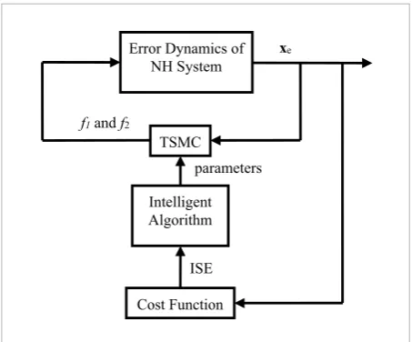
The error dynamics of the NH system reach zero in a finite period of time if the parameters are designed properly. Therefore, the design parameters should be chosen carefully, otherwise, it may take very long time for tracking error to reach zero or tracking er-ror may fluctuate with the amplitude around zero without reaching it, as it will be shown in simulation results presented in Section 5. We separately utilize four intelligent optimization algorithms, namely, DE, BO, BFO and CO to design these parameters such that an enhanced tracking error can be achieved. Figure 1 shows the block diagram of the main problem.

Figure 1

A block diagram of the proposed method.

Error Dynamics of NH System

Intelligent Algorithm TSMC

xe

parameters

Cost Function

f1 and f2

ISE

In this paper, our goal is to design the parameters p_i, i

q (i=1,...,n),β_i (i=1,...,n−1) and k2 considering the constraints mentioned above for each parameter by using evolutionary algorithms such that the tracking errors reach zero in finite time. In the following subsec-tions, it will be illustrated how such algorithms work. 3.3.1. Differential Evolution (DE) Algorithm DE algorithm has been proposed by Storn and Price in 1995 [31]. They have used this algorithm to solve continuous optimization problems, and recently it has been used for integer, discrete and other type of engineering problems. This algorithm has many sim-ilarities with other intelligent algorithms, such as

ge-netic algorithm (GA). However, the main difference is its exclusive way to produce new population.

Three main operators in this algorithm are crossover, mutation and selection. DE algorithmchanges the or-dering of operators used in this algorithm. In addition, the way of using mutation is exclusive. The algorithm is explained in the following order:

Parameter Selection. The problem formulation in-cludes the objective function, the unknown variables or parameters and decision parameters which have to be defined at the first stage. The ranges of unknown parameters have to be also determined. In addition, the parameters of the algorithm such as the popula-tion size and scaling as well as crossover factors have to be chosen.

Initialization. The initial population with Np vectors

is produced randomly in the acceptable range defined for parameters:

, , (0,1) ( , , )

for 0,1,..., 1

j g j L j j U j L

p

rand

j N

= + × −

= −

x b b b

(31)

where bj,L and bj,U are lower and upper limit vectors for

unknown parameters, respectively. xj,g is the base

vec-tor, g denotes the generation and randj(0,1) produces

a random number with normal distribution in the in-terval of (0,1].

Mutation. Differential mutation is a difference vec-tor that is being sampled randomly from the initial population. If vi is the target vector, the mutation

vec-tor is produced with the following equation:

0 1 2

, , ( , , ),

i g = r g + ×F r g− r g

v x x x (32)

where x_{r g0,} (base vector) and x_{r g1,} −x_{r g2,} (difference vector) are selected randomly from initial population considering r0≠r1≠r2≠i. Moreover, F is a scaling

fac-tor which is a strictly positive real number that varies in the interval (0 , 1].

Crossover. Each current vector combines with muta-tion vector and produces a new temporary response. In this paper, we use uniform crossover with the fol-lowing equation:

, rand

, ,

if (0,1) or

, O.W.

j g j r

j g j g

rand ≤C j= j

 =  

v

where Cr∈ [0 , 1] is user defined crossover

probabil-ity and uj,g is called trial vector. In fact, (33) implies

that trial vector is constructed at the randomly cho-sen parameter index, jrand, which implies that the

tri-al vectors are inherited from the mutant vector until

randj (0,1) ≤Cr. The first time that randj (0,1) ≤Cr, all

the remaining parameters are obtained from the tar-get vector.

Selection. We select the next generation with the fol-lowing equation. It means that if the value of the ob-jective function, evaluated with the trial vector, was better than the one evaluated with the target vector, in the next generation, the target vector is replaced with the trial vector, otherwise we keep the previous one:

, , ,

, 1 ,

if ( ) ( )

, O.W.

j g j g j g

j g

j g

f f

+

≤ 

=  

u u x

x _x (34)

where f denotes the objective function.

Termination Criteria. Many conditions can be used for stopping the algorithm. In this paper, we used a stopping criterion based on maximum iteration (gmax).

3.3.2. Bat Optimization (BO) Algorithm

Another subcategory of swarm intelligence algo-rithms is BO algorithm that has been presented by Yang in 2010 [39]. This algorithm has been proposed based on the sound reflection of special groups of bats called micro-bats that have forearm length be-tween 2.2-11 centimeters. These bats can find their prey even in environmentswith complete darkness. They send out a very loud sound pulse and listen the echo returning from the surrounding objects. Usual-ly, it takes about 300-400 microseconds to integrate the received signals. They follow louder sounds when they are looking for prey. The complete steps of the BO algorithm in simulation are described as follows: Step1. Initialize the number of bats (n), decision variable (d), initial velocity vector (vi), define

admissi-ble interval for frequency [fmin, fmax], allocate the initial

loudness, A0, in (1, 2) and initial emission rate, r0, in (0,

1), for each bat and also produce initial bat population vector xi in search space randomly as:

low rand( high low).

i = + −

x x x x (35)

Step2. Evaluate objective function and determine the global best, xbest.

Step3. Update the frequency, velocity and position:

min max min

best

( )

( )

,

i

i i i i

i i i

f f f f

f

β

= + −

= + −

= +

v v x x

x x v

(36)

where β∈ [0, 1] is a random number.

Step4. Produce a random number (rand) with uni-form distribution between 0 and 1. If rand > ri, then do

local search, i.e.:

new = old +ε ,

x x A (37)

where ε∈ [-1, 1] and A is the average loudness of all the bats at this time step.

Step5. Evaluate the objective function.

Step6. Produce a random number (rand) with uni-form distribution between 0 and 1. If rand < Aj and f(xnew) < f(xbest), then accept the new solution and

up-date Ai, ri as:

[1 exp( )],

i i

i i

A A

r r t

α

γ =

= − − (38)

where 0 < α < 1 and γ > 0 are constant values.

If the above condition is not satisfied, rank the bats and find the best one.

Step7. Check the termination criteria. If it is not sat-isfied, go to step 3.

Step8. End.

3.3.3. Bacterial Foraging Optimization (BFO) Algorithm

BFO is an optimization algorithm based on swarm in-telligence that has been presented by Passino in 2001 to solve continuous optimization problems [28]. The main idea of this algorithm is based on natural selec-tion which actually tends to eliminate animals with poor “foraging strategies” and also spread those genes of animals that have successful foraging strategies. After many generations, poor foraging strategies were either eliminated or got better.

gov-erned by four processes, namely, chemotaxis, swarm-ing, reproduction and elimination-and-dispersal. All the steps of this algorithm are explained as follows: Initialization: In this step, the parameters of the al-gorithm, i.e., s, p, Ns, Nc, Nre, Ned, pedthat are respectively

the number of bacteria, problem dimensions, number of swims, number of chemotactic steps, reproduction steps, elimination-dispersal steps, elimination-dis-persal probability are initialized. Moreover, C(i), for

i=1,2,…,s, is defined as chemotactic step size of each bacteria and θi is considered as initial position of all

bacteria.

Main Loop: The main loop consists of the following steps:

Step1. Elimination-dispersal loop: l = l + 1, Step2. Reproduction loop: k = k + 1, Step3. Chemotactic loop: j = j + 1,

Step4. For each bacterium, i = 1, 2, … , s take the che-motactic step as follows:

_ Calculate the evaluation function and add the

attractant effect to the nutrient concentration:

(

)

last

( , , , ) ( , , , )

( , , ), ( , , ) ( , , , ),

cc i

J i j k l J i j k l

J j k l P j k l

J J i j k l

θ = + =

(39)

where J is the objective function that has to be minimized, and Jcc is the cell-to-cell attractant

ef-fect to the nutrient concentration. In addition, P

represents the position of each member in the pop-ulation of s bacteria at the j-th chemotactic step,

k-th reproduction step, and l-th elimination-dis-persal event.

_ Tumble: Generate a random vector, D(i), on [-1, 1].

_ Move: Obtain new position by:

( ) ( 1, , ) ( , , ) ( ) .

( ) ( )

i j k l i j k l C i _T i

i i

θ + =θ + D

D D (40)

_ For this position, evaluate the objective function

J(i, j+1, k, l).

_ Swim:

Let m = 0 (counter for swim length). While m < Ns:

Let m = m + 1.

If moving condition is satisfied, i.e.,

J(i, j+1, k, l) < Jlast, then move and let Jlast=J(i,j+1,k,l).

Otherwise and also if m=Ns, swimming loop is done.

_ If i ≠ s, go to the next bacterium and repeat the above steps.

_ If j < Ns, go to step 3; otherwise moving loop ends.

Step5. Reproduction:

a For the given k, l and for each bacterium, sort

bac-teria based on the objective evaluation function.

b A half of the bacteria with worst value dies and

the other half with better value is divided into two parts in the same position.

c If k < Nre, go to step 2.

d Otherwise, end the reproduction loop.

Step6. Elimination-dispersal loop: l = l + 1.

a If condition of elimination and dispersal is

satis-fied, the bacterium is eliminated and replaced with another bacterium that is produced randomly.

b If l < Ned, go to step 1.

c Otherwise, end the elimination-dispersal loop.

3.3.4. Cuckoo Optimization (CO) Algorithm In 2009, research about cuckoo search has been de-veloped by Yang and Deb [40]. Since then, CO algo-rithm has been presented by Rajabioun in 2011 [30]. The main reason that motivates researches to devel-op this devel-optimization algorithm is that cuckoo has a different life style in comparison with other birds. CO algorithm starts with random initial population simi-lar to the other optimization algorithms. Each cuckoo lays a random number of eggs. Hence, the population is divided into two types, cuckoos and eggs. Some kind of effort occurs between this population and the bet-ter cuckoos survive in this competition. These betbet-ter cuckoos immigrate to a better environment, start re-production and laying eggs. This cycle continues until the stopping criteria are satisfied. Steps of this algo-rithm are as follows:

Step1. Generate the initial habitats for cuckoos ran-domly in the search space.

hi low

Number of current cuckoo's eggs

Total number of eggs (var var ),

ELR=α ×

× −

(41)

where varhi and varlow are, respectively, the upper and

lower limits of decision variables and α is an integer used to handle the maximum value of ELR.

Step4. Each cuckoo lays a random number of eggs in other host birds’ nest inside its corresponding ELR. Step5. Those eggs that are verified because of lesser similarity to the host birds’ eggs will be killed by the host birds.

Step6. Let eggs hatch and grow. The first-born cuck-oo ruins other eggs because of its three times larger body; it eats more food and other chicks die from star-vation. Hence, we have only one cuckoo remaining in each nest in the end.

Step7. Evaluate the habitat of each newly grown cuckoo.

Step8. Determine the maximum number of cuckoos that can live in each environment and kill those that live in the worst habitats.

Step9. Cluster cuckoos, find the best group and se-lect the best of it as a target habitat.

Step10. Immigrate toward the target habitat:

next = current +F( goal− current),

x x x x (42)

where F is a parameter defined between 0 and 1. Step11. If stopping condition is not satisfied, go to Step 2.

Step12. End.

3.3.5. Parameters for Adjustment

To determine the parameters of terminal sliding surface with intelligent optimization algorithms, we firstly put all the parameters needed to be designed in the following vector:

1 2 1 2 1 1

[ , ,...., n , , , ,..., , ].n n

Param = β β β ₋ k q p q p ₍₄₃₎

The algorithms firstly randomly produce the initial population. Each member of the population contains the vector above. Parameters in the vector must satis-fy the constraints, in which pi and qi (i = 1, 2, … , n) are

odd positive integers such that qi < pi and βi (i = 1, 2, … , n-1) and k2 are certain positive constants. For each set

of parameters shown in the form of the vector above, we can define the control law f2 as in (17). By applying

the control law to the system, error tracking dynam-ics (xie, for i = 2, 3, ... , n) can be obtained. Having these

errors, we can define the integral square error (ISE) as an objective function with the following equation:

0

n 2

2

ISE t( ie( )) .

i t

x d

In order to choose the parameters that are deter-mined by the intelligent optimization algorithm, we make a change in this objective function. For tracking purposes, occurring peaks at the beginning are preva-lent, while peaks at the end are not desirable. In order to avoid the integration of these two peaks in the ob-jective function, they should be separated. Therefore, we consider the integration of the square error from a short time after the beginning. In fact, for simulation, we take t0 = 0.4 and t = 10 in (44).

The value of ISE obtained from (44) is allocated to each parameter vector. It is obvious that the vector with less value of the allocated ISE is more successful in the algorithm. We continue the algorithm until the algorithm gets us the parameter vector with the best objective function value.

4. Mathematical Model of Wheeled

Mobile Robots (WMRs)

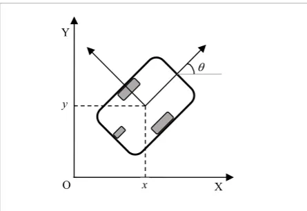
WMRs are one of the applications of the NH systems which are especially being used in environments in which a motion on smooth surfaces such as shopping centers, hospitals and industrial areas is needed. Fur-thermore, it plays an important role in security, trans-portation inspecting, painting, soccer playing robots and other aspects. In fact, the main control problem in such systems is to force systems to move along a de-sired trajectory. In this paper, a nonholonomic WMR with two driving wheels and one passive wheel in its behind is considered, as shown in Figure 2.

slipping. In other words, the WMR can only move in a direction which is perpendicular to the axis of the driving wheels. Therefore, we have:

sin cos 0,

x θ−y θ = (45)

where [_{x yθ}]T_{represents the position of the WMR in} the Cartesian space.

It has been well known that, under the assumption of pure rolling, state space equations of WMR with two driving wheels and a passive wheel in the behind is described by:

1 1

2

sin 0 cos 0 0 1

,

x

v y

T v

M T θ θ

ω θ

ω −

−

   

 

  ₌ 

 

   _{  }

   

   

   

= _{ }

 

   

  

 

(46)

where v is the linear velocity of the wheel and ω is the angular velocity around the vertical axis. M is a sym-metric positive matrix. T₁ is the pushing force in the direction of heading angle and T₂ is the torque about the vertical axis for steering. It is assumed that v and

ω are the available control inputs, which can be easily calculated from torques of the motor driving wheels. In order to use the proposed TSMC design method, we convert the equations of the system into extended chained form of the NH systems considering the fol-lowing states and control transformation:

Figure 2

A nonholonomic WMR with two driving wheels and a passive wheel

X

x

 Y

O

y

1

2

3

1

2 3

sin cos

cos sin

,

x

x x y

x x y

u

u v x

θ

θ θ

θ θ

ω ω =

= − +

= +

= = −

(47)

where ( , )x x2 3 denotes the coordinates of the center of mass, x₂is the axis aligned with the vehicle orien-tation. Moreover, u₁ and u₂are the control inputs which depend on the pushing force T1, steering torque

2

T and linear and angular velocity as defined in (48):

1 1 1 2

3

2 2 2

0 1 0

. 1

u T

M

x

u T x ω

−

 

     

=_{ } +

  ₋   ₋ 

       



 (48)

Using above definition, state space equations can be described as:

1 1

2 2

3 2 1

1 1

2 2,

x u

x u

x x u

u f

u f

= = = = =

    

(49)

where f₁ and f₂ are the adjustable control inputs of the dynamical model. These third order equations illustrate a NH system in the extended chained form same as equation (1) with n=3. Now assume that the desired trajectory for the third-order NH system,

1 2 3

[ , , ]T

d d d d

x = x x x , is generated by:

1 1

2 2

3 2 1 ,

d d

d d

d d d

x u

x u

x x u

= = =

  

(50)

where u1d and u2d are the reference controls.

Fur-thermore, we denote the tracking error as x_e = −x x_d where x is the state vector. Tracking error for the third-order NH system, considering the dynamic ex-tension, satisfies the following equations:

1 1 1

2 2 2

3 2 1 2 1 1

1 1 1

2 2 2

( )

.

e d

e d

e e d d

x u u

x u u

x x u x u u

u f f

u f f

= −

= −

= + −

= + D

= + D

    

The first subsystem is controlled by f₁ as defined in (7). In the proposed method, the control task is to de-signf₂, as (17), using the intelligent TSMC method such that tracking error becomes zero in finite time. By using contexts stated in Section 3 for controlling second subsystem of generalized NH systems in ex-tended chained form (51), system assuming y₁=x_3e,

2 2e

y =x and y₃=u u₂− ₂d, we should convert the

equa-tions of third-order NH into the following equaequa-tions: 1 1 2

2 3

3 2 2.

d

y u y

y y

y f f

= =

= + D

  

(52)

To solve these equations, we consider terminal slid-ing surface as:

1 1

2 2

0 1

1 0 1 0

2 1 2 2 q

p

q

p

s y

s s s

s s s

β β =

= +

= +





(53)

and the control input as:

3 3

1 1 2 2

2

/

/ /

2 1 2 0 2 1 2 2

1

1 [ ( q p) ( q p) ( q p)].

d

d d

f s s k s

u β dt β dt

= − + + ₍₅₄₎

The simulation results in the next section show that if we design parameters using intelligent optimization algorithms, then the tracking errors will reach and re-main on zero in a short period of time.

5. Simulation Results

In this section, we show the results of computer sim-ulation performed in MATLAB/SIMULINK. The de-sired trajectory is described as follows:

(sin cos ) (sin cos ) .

d

d

d

x t t t

y t t t

t θ

= +

= −

=

(55)

For the first subsystem described by (20), by consid-ering disturbance as Δf1= 0.1sin(t), the control law of

the form (7) with parameters q q= ′=3, p p= ′=5,

and β = =k₁ 3has been applied to the system and the

results have been shown in Figure 3. It can be seen that, using the defined control law in (7), the tracking errorx_1e reaches zero in a few seconds and the input

1

u reaches the desired value in a finite time as well. In Figure 4, the trajectory errors x_2e andx_3e, the in-put u₂ and control law f₂ for the second subsystem (52) have been shown when the parameters of termi-nal sliding surface are selected randomly and with-out using the intelligent algorithms. The parameters assumed in this simulation are q1=45, p1=117, q2=23, p2=123, q3=3, p3=5, β1=26, β2=54, and k2=44. It can be

observed that for the case that the parameters of ter-minal sliding surface are determined properly, the tracking error reaches zero in a finite time and it may fluctuate around zero with high amplitude.

Figure 3

a) Tracking error of x1e, input u1 of first subsystem (5), b) control law f1 defined in (7)

0 2 4 6 8 10

-1.5 -1 -0.5 0 0.5 1 1.5 2 2.5 3

Time(second)

0 2 4 6 8 10

-10 -8 -6 -4 -2 0 2 4 6

Time(second) f1

x_1e u₁

Information Technology and Control 2018/1/47 38

Figure 4

a) Tracking error of x2e, b) tracking error of x3e, c) dynamic control law u2 and d) WMR linear velocity v when the parameters of terminal sliding surface structure are selected randomly

11

0 2 4 6 8 10

-1.5 -1 -0.5 0 0.5 1 1.5 2 2.5 3

Time(second)

0 2 4 6 8 10

-10 -8 -6 -4 -2 0 2 4 6

Time(second)

f1

a) _b)

x_1e u₁

Figure 3. a) Tracking error of x1e, input u1 of first subsystem (5), b) control law f1 defined in (7).

0 0.5 1 1.5 2

-40 -20 0 20

Time (second)

x 2e

0 0.5 1 1.5 2

-1 0 1 2

Time (second)

x 3e

0 0.5 1 1.5 2

-2000 -1000 0 1000 2000

Time (second) u2

0 0.5 1 1.5 2

-4 -2 0 2x 10

5

Time (second)

v

a

c d

b

Now, we apply each algorithm presented in Section 3 to find the parameters of the terminal sliding mode surface structure proposed to control the second subsystem of WMR. For each algorithm, in order to compare the performance of the algorithms, the same objective function is used which is integral square er-ror, ISE, defined in (44). Each algorithm needs its own preliminary parameters to be defined. These parame-ters are taken into consideration as discussed below: DE: For simulation use, the population size is as-sumed as 50, and the scaling factor is considered ran-domly in the range of 0.2 < F < 0.8 with uniform distri-bution. We additionally take Cr = 0.2 as the crossover

probability.

BFO: For this algorithm, we assume that s = 50, Nc =

10, Ns = 4, Nre = 4, Ned = 2 and Ped = 0.25.

BO: We use 30 bats with fmin = 0, fmax = 2. Other parameters

are selected randomly in the range stated in Section 3. CO: For simulating this algorithm, a number of 20 cuckoos is used. There are between two to five eggs. For clustering, we use k-nearest-neighborhood

(KNN) clustering method with three clusters. In ad-dition, we take α = 5, F = 9.

Considering disturbance for the second subsystem de-fined in (51) as Δf2= sin(t), simulation results of

a

c d

b Figure 5

a) Tracking error of x2e, b) tracking error of x3e, c) dynamic control law u2 and d) WMR linear velovity v when the parameters of the proposed method are selected using intelligent algorithms

Figure 6

Control input f2 when the parameters of TSMC are selected using intelligent algorithms

H. Ghasemi, B. Rezaie and Z. Rahmani

0 0.2 0.4 0.6 0.8 1

-60 -40 -20 0 20

x2e

0 0.2 0.4 0.6 0.8 1

-0.5 0 0.5 1 1.5 2

Time (second)

x 3e

DE CO BO BFO

0 0.2 0.4 0.6 0.8 1

-2000 -1000 0 1000 2000

Time (second) u2

0 0.2 0.4 0.6 0.8 1

-2 0 2 4 6

Time (second)

v

DE CO BO BFO

DE CO BO BFO

DE CO BO BFO

Time(second)

Figure 5. a) Tracking error of x2e, b) tracking error of x3e, c) dynamic control law u2 and d) WMR linear velovity v when the parameters of the proposed method are selected using intelligent algorithms.

0.4 0.6 0.8 1 1.2 1.4 1.6 1.8 2

-3000 -2000 -1000 0 1000 2000 3000

Time (second)

f2

DE CO BO BFO

H. Ghasemi, B. Rezaie and Z. Rahmani

0 0.2 0.4 0.6 0.8 1

-60 -40 -20 0 20

x2e

0 0.2 0.4 0.6 0.8 1

-0.5 0 0.5 1 1.5 2

Time (second)

x 3e

DE CO BO BFO

0 0.2 0.4 0.6 0.8 1

-2000 -1000 0 1000 2000

Time (second)

u 2

0 0.2 0.4 0.6 0.8 1

-2 0 2 4 6

Time (second)

v

DE CO BO BFO

DE CO BO BFO

DE CO BO BFO

Time(second)

c)

b)

d) a)

Figure 5. a) Tracking error of x2e, b) tracking error of x3e, c) dynamic control law u2 and d) WMR linear velovity v when the

parameters of the proposed method are selected using intelligent algorithms.

0.4 0.6 0.8 1 1.2 1.4 1.6 1.8 2

-3000 -2000 -1000 0 1000 2000 3000

Time (second)

f 2

Table 1

The results of using intelligent algorithms with or without disturbance for WMR. Parameters are a vector with the form of [β1, β2, k2, q1, p1, q2, p2, q3, p3] that shows the simulation outputs of the algorithms

Algorithm NFE Time Best Cost Best Parameters

CO 3516 52 min 0.01138 [21.7, 10.6, 1.6, 49, 41, 65, 97,9, 39]

DE 2050 40 min 0.01139 [11.7, 20.8, 1, 177, 217, 169, 197, 5, 271]

BO 1230 24 min 0.0119 [14.3, 15, 54.1, 275, 299, 235, 267, 113, 177 ]

BFO 8000 3 h 54 min 0.04 [22, 16, 148, 219, 261, 219, 261,5, 131]

converge to zero very quickly in less than a second. In addition, the control effort has been reduced by using the intelligent control scheme.

Figure 7

Tracking the desired trajectory of x by four algorithms

Figure 8

Tracking the desired trajectory of y by four algorithms

In order to see how tuning parameters affects the tra-jectory tracking, Figures 7 to 10 show the effectiveness of each algorithm in tracking the desired trajectory. It

13

0.5 1 1.5 2 2.5 3

-3 -2 -1 0 1 2 3

Time (second)

x

Desired Trajectory BFO DE CO BO

Figure 7. Tracking the desired trajectory of x by four algorithms.

0.5 1 1.5 2 2.5 3

-2 -1 0 1 2 3 4

Time (second)

y

Desired Trajectory DE CO BO BFO

Figure 8. Tracking the desired trajectory of y by four algorithms.

13

0.5 1 1.5 2 2.5 3

-3 -2 -1 0 1 2 3

Time (second)

x

Desired Trajectory BFO DE CO BO

Figure 7. Tracking the desired trajectory of x by four algorithms.

0.5 1 1.5 2 2.5 3

-2 -1 0 1 2 3 4

Time (second)

y

Desired Trajectory DE CO BO BFO

Figure 9

Tracking the desired trajectory of θ by four algorithms

Figure 10

Trajectory tracking of WMR in Cartesian coordinate using four intelligent algorithms a) BFO, b) BO, c) DE, d) CO

0 0.5 1 1.5 2 2.5 3 3.5 4 4.5 5

0 0.5 1 1.5 2 2.5 3 3.5 4 4.5 5

Time (second)



Desired Trajectory Four Algorithms

Figure 9. Tracking the desired trajectory of  by four algorithms.

-15 -10 -5 0 5 10 15

-15 -10 -5 0 5 10 15

x

y

Trajectory BO TSM

-15 -10 -5 0 5 10 15

-15 -10 -5 0 5 10 15

x

y

Trajectory DE TSM

-15 -10 -5 0 5 10 15

-15 -10 -5 0 5 10 15

x

y

Trajectory CO TSM

-15 -10 -5 0 5 10 15

-15 -10 -5 0 5 10 15

x

y

Trajectory BFO TSM

d) b) a)

c)

0 0.5 1 1.5 2 2.5 3 3.5 4 4.5 5

0 0.5 1 1.5 2 2.5 3 3.5 4 4.5 5

Time (second)



Desired Trajectory Four Algorithms

Figure 9. Tracking the desired trajectory of  by four algorithms.

-15 -10 -5 0 5 10 15

-15 -10 -5 0 5 10 15

x

y

Trajectory BO TSM

-15 -10 -5 0 5 10 15

-15 -10 -5 0 5 10 15

x

y

Trajectory DE TSM

-15 -10 -5 0 5 10 15

-15 -10 -5 0 5 10 15

x

y

Trajectory CO TSM

-15 -10 -5 0 5 10 15

-15 -10 -5 0 5 10 15

x

y

Trajectory BFO TSM

a b

0.2 0.4 0.6 0.8 1 -10

-5 0 5

Time (second)

x_1e

x_2e

x_3e

0 1 2 3 4 5

-10 -5 0 5

Time (second)

x

x_d

0 1 2 3 4 5

-15 -10 -5 0 5

Time (second)

y

y_d

0 0.5 1 1.5 2 2.5

0 0.5 1 1.5 2 2.5

Time (second)

 d

can be seen from these figures that using the parame-ters of TSMC obtained from BFO and BO algorithms, the desired trajectory is tracked with a little fluctua-tion. However, using DE and CO algorithms, the pa-rameters are properly tuned and therefore the trajec-tory is accurately tracked in a short period of time. Simulation results show that among these four al-gorithms, by using CO algorithm, the best parame-ter values can be obtained for trajectory tracking of

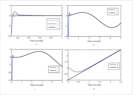
WMR. Table 1 also reveals that BFO leads to a greater objective function and it takes much time compared with the others. Therefore, it could not find the best parameter values. However, CO algorithm tunes the parameters of terminal sliding surface such that leads to the least ISE as objective function. Thus, it can be concluded that CO algorithm is the best algorithm for tuning these parameters. The tracking error and the state variables, when CO algorithm is used for select-ing the parameters, have been shown in Figure 11.

a _b

c d

Figure 11

a) Error of transformed system x1e, x2e, x3e, b) tracking of desired trajectory x, c) tracking of desired trajectory y, d) tracking

of desired trajectory θ when the parameters of terminal sliding surface are selected using CO algorithm

6. Conclusion

In this paper, an intelligent TSMC has been proposed for controlling the NH systems in extended chained form. In this method, intelligent algorithms have been used to determine the parameters of the recursive

for designing the parameters. It has been shown that, using these intelligent algorithms, appropriate param-eters can be found such that the system can track the desired trajectory very well. Simulation results per-formed on WMR as a benchmark of the NH systems have shown the effectiveness of the proposed design for error dynamic tracking even in the presence of the input disturbance. In addition, simulation results

show that CO algorithm has provided the most effec-tive tuning of parameters among other algorithms such that the tracking error can reach zero in a very short period of time with a small amount of chattering.

Acknowledgments

We would like to present our thanks to anonymous re-viewers for their helpful suggestions.

References

1. Astolfi, A. Discontinuous Control of Nonholonomic Systems. Systems and Control Letters, 1996, 27(1), 37-45. https://doi.org/10.1016/0167-6911(95)00041-0 2. Binazadeh, T., Shafiei, M. H. Nonsingular Terminal

Sliding-Mode Control of a Tractor–Trailer System. Sys-tems Science and Control Engineering, 2014, 2(1), 168-174. https://doi.org/10.1080/21642583.2014.890552 3. Bloch, A. M. Nonholonomic Mechanics and

Con-trol. Springer-Verlag, New York, 2003. https://doi. org/10.1007/b97376

4. Brockett, R. W. Asymptotic Stability and Feedback Sta-bilization. In: Brockett R. W., Millman R. S., Sussmann H. J. (Eds.), Differential Geometric Control Theory, Birkhauser, Boston, 181-191, 1983.

5. Chen, C. Y., Li, T. H. S., Yeh, Y. C. EP-Based Kinematic Control and Adaptive Fuzzy Sliding-Mode Dynam-ic Control for Wheeled Mobile Robots. Informa-tion Sciences, 2009, 179(1-2), 180-195. https://doi. org/10.1016/j.ins.2008.09.012

6. Chen, N., Song, F., Li, G., Sun, X., Ai, C. S. An Adaptive Sliding Mode Backstepping Control for the Mobile Ma-nipulator with Nonholonomic Constraints. Communi-cations in Nonlinear Science and Numerical Simula-tion, 2013, 18(10), 2885-2899. https://doi.org/10.1016/j. cnsns.2013.02.002

7. Chen, S. Y., Lin, F. J. Robust Nonsingular Terminal Sliding-Mode Control for Nonlinear Magnetic Bearing System. IEEE Transactions on Control Systems Tech-nology, 2011, 19(3), 636-643. https://doi.org/10.1109/ TCST.2010.2050484

8. Fang, Y., Yuan, Z., Fei, J. Adaptive Fuzzy Backstepping Con-trol of MEMS Gyroscope Using Dynamic Sliding Mode Approach. Information Technology and Control, 2015, 44(4), 380-386. https://doi.org/10.5755/j01.itc.44.4.9110 9. Ferrara, A., Giacomini, L., Vecchio, C. Control of

Non-holonomic Systems with Uncertainties via Second-Or-der Sliding Modes. International Journal of Robust and Nonlinear Control, 2008, 18(4-5), 515-528. https://doi. org/10.1002/rnc.1202

10. Jiang, Z. P. Robust Exponential Regulation of Non-holonomic Systems with Uncertainties. Automatica, 2000, 36(2), 189-209. https://doi.org/10.1016/S0005-1098(99)00115-6

11. Jin, M., Lee, J., Chang, P. H., Choi, C. Practical Nonsin-gular Terminal Sliding-Mode Control of Robot Ma-nipulators for High-Accuracy Tracking Control. IEEE Transactions on Industrial Electronics, 2009, 56(9), 3593-3601. https://doi.org/10.1109/TIE.2009.2024097 12. Khooban, M. H. Design an Intelligent Proportional-De-rivative (PD) Feedback Linearization Control for Non-holonomic-Wheeled Mobile Robot. Journal of Intelli-gent and Fuzzy Systems, 2014, 26(4), 1833-1843. 13. Kocamaz, U. E., Göksu, A., Taşkın, H., Uyaroğlu, Y.

Synchro-nization of Chaos in Nonlinear Finance System by Means of Sliding Mode and Passive Control Methods: A Compar-ative Study. Information Technology and Control, 2015, 44(2), 172-181. https://doi.org/10.5755/j01.itc.44.2.7732 14. Kolmanovsky, I., McClamroch, N. H.

Develop-ments in Nonholonomic Control Problems. IEEE Control Systems, 1995, 15(6), 20-36. https://doi. org/10.1109/37.476384

15. Lee, T. H., Lam, H. K., Leung, F. H. F., Tam, P. K. S. A Prac-tical Fuzzy Logic Controller for the Path Tracking of Wheeled Mobile Robots. IEEE Control Systems, 2003, 23(2), 60-65. https://doi.org/10.1109/MCS.2003.1188772 16. Liang, Z. Y., Wang, C. L. Robust Stabilization of Non-holonomic Chained form Systems with Uncertainties. Acta Automatica Sinica, 2011, 37(2), 129-142.

17. Liu, Y. L., Wu, Y. Q. Output Feedback Control for Sto-chastic Nonholonomic Systems with Growth Rate Re-striction. Asian Journal of Control, 2011, 13(1), 177-185. https://doi.org/10.1002/asjc.230

19. Man, Z., Yu, X. H. Terminal Sliding Mode Control of MIMO Linear Systems. IEEE Transactions on Circuits and Sys-tems I: Fundamental, Theory and Applications, 1997, 44(11), 1065-1070. https://doi.org/10.1109/81.641769 20. Marchand, N., Alamir, M. Discontinuous Exponential

Stabilization of Chained form Systems. Automatica, 2003, 39(2), 343-348. https://doi.org/10.1016/S0005-1098(02)00229-7

21. Mobayen, S. Finite-Time Tracking Control of Chained-Form Nonholonomic Systems with External Distur-bances Based on Recursive Terminal Sliding Mode Method. Nonlinear Dynamics, 2015, 80, 669-683. https://doi.org/10.1007/s11071-015-1897-4

22. Mon, Y. J., Lin, C. M. ANFIS-Based Integral Terminal Sliding Mode Control for Disturbed Chaotic System. Journal of Intelligent and Fuzzy Systems, 2014, 27(1), 443-450.

23. Mon, Y. J., Lin, C. M. Double Inverted Pendulum Decou-pling Control by Adaptive Terminal Sliding-Mode Re-current Fuzzy Neural Network. Journal of Intelligent and Fuzzy Systems, 2014, 26(4), 1723-1729.

24. Ou, M., Du, H., Li, S. Finite-Time Tracking Control of Multiple Nonholonomic Mobile Robots. Journal of Franklin Institute, 2012, 349(9), 2834-2860. https:// doi.org/10.1016/j.jfranklin.2012.08.009

25. Pan, Y., Liu, Y., Xu, B., Yu, H. Hybrid Feedback Feedfor-ward: An Efficient Design of Adaptive Neural Network Control. Neural Networks, 2016, 76(6), 122-134. https:// doi.org/10.1016/j.neunet.2015.12.009

26. Pan, Y., Yu, H. Biomimetic Hybrid Feedback Feedfor-ward Neural-Network Learning Control. IEEE Trans-actions on Neural Networks and Learning Systems, 2016, 28(6), 1481-1487. https://doi.org/10.1109/TNN-LS.2016.2527501

27. Pan, Y., Yu, H., Er, M. J. Adaptive Neural PD Control with Semiglobal Asymptotic Stabilization Guarantee. IEEE Transactions on Neural Networks and Learning Sys-tems, 2014, 25(12), 2264-2274. https://doi.org/10.1109/ TNNLS.2014.2308571

28. Passino, K. M. Biomimicry of Bacterial Foraging for Distributed Optimization and Control. IEEE Control Systems, 2002, 22(3), 52-67. https://doi.org/10.1109/ MCS.2002.1004010

29. Ploeg, J., Schouten, H. E., Nijmeijer, H. Position Con-trol of a Wheeled Mobile Robot Including Tire Behav-ior. IEEE Transactions on Intelligent Transportation Systems, 2009, 10(3), 523-533. https://doi.org/10.1109/ TITS.2009.2026316

30. Rajabioun R. Cuckoo Optimization Algorithm. Applied Soft Computing, 2011, 11(8), 5508-5518. https://doi. org/10.1016/j.asoc.2011.05.008

31. Storn, R., Price, K. Differential Evolution – A Simple and

Efficient Heuristic for Global Optimization over Contin-uous Spaces. Journal of Global Optimization, 1997, 11, 341-359. https://doi.org/10.1023/A:1008202821328 32. Sun, T., Pei, H., Pan, Y., Zhou, H., Zhang, C. Neural

Net-work-Based Sliding Mode Adaptive Control for Robot Manipulators. Neurocomputing, 2011, 74(14-15), 2377-2384. https://doi.org/10.1016/j.neucom.2011.03.015 33. Tian, Y. P., Li, H. Exponential Stabilization of

Nonho-lonomic Dynamic Systems by Smooth Time-Varying Control. Automatica, 2002, 38(7), 1139-1146. https:// doi.org/10.1016/S0005-1098(01)00303-X

34. Wu, Y., Wang, B., Zong, G. D. Finite-Time Tracking Controller Design for Nonholonomic Systems with Ex-tended Chained Form. IEEE Transactions on Circuits and Systems II: Express Briefs, 2005, 52(11), 798–802. https://doi.org/10.1109/TCSII.2005.852528

35. Wu, Y., Yu, X., Man, Z. Terminal Sliding Mode Con-trol Design for Uncertain Dynamic Systems. Systems and Control Letters, 1998, 34(5), 281-287. https://doi. org/10.1016/S0167-6911(98)00036-X

36. Wu, Y. Q., Zhu, C. L., Zhang, Z. C. Finite-Time Stabiliza-tion of a General Class of Nonholonomic Dynamic Sys-tems via Terminal Sliding Mode. International Journal of Automation and Computing, 2016, 13(6), 585-595. https://doi.org/10.1007/s11633-015-0931-9

37. Xi, Z. R., Feng, G., Jiang, Z. P., Cheng, D. Output Feed-back Exponential Stabilization of Uncertain Chained Systems. Journal of Franklin Institute, 2007, 344(1), 36-57. https://doi.org/10.1016/j.jfranklin.2005.10.002 38. Xu, W. L., Huo, W. Variable Structure Exponential

Sta-bilization of Chained Systems Based on the Extended Nonholonomic Integrator. Systems and Control Let-ters, 2000, 41(4), 225-235. https://doi.org/10.1016/ S0167-6911(00)00057-8

39. Yang, X. S. A New Metaheuristic Bat-Inspired Algorithm. In: Gonzalez, J. R., Pelta, D. A., Cruz C., Terrazas, G., Kras-nogor, N. (Eds.) Nature Inspired Cooperative Strategies for Optimization (NICSO 2010), Springer, Berlin, 65-74, 2010. https://doi.org/10.1007/978-3-642-12538-6_6 40. Yang, X. S., Deb, S. Engineering Optimization by Cuckoo

Search. International Journal of Mathematical Model-ing and Numerical Optimization, 2010, 1(4), 330-343. https://doi.org/10.1504/IJMMNO.2010.035430 41. Yu, X., Man, Z. Model Reference Adaptive Control

Systems with Terminal Sliding Modes. International Journal of Control, 1996, 64(6), 1165-1176. https://doi. org/10.1080/00207179608921680