Partial differential equations for 3D Data compression and Reconstruction

Partial differential equations for 3D Data compression and

Reconstruction

RODRIGUES, Marcos <http://orcid.org/0000-0002-6083-1303>, OSMAN,

Abdusslam and ROBINSON, Alan

Available from Sheffield Hallam University Research Archive (SHURA) at:

http://shura.shu.ac.uk/6780/

This document is the author deposited version. You are advised to consult the

publisher's version if you wish to cite from it.

Published version

RODRIGUES, Marcos, OSMAN, Abdusslam and ROBINSON, Alan (2013). Partial

differential equations for 3D Data compression and Reconstruction. ADSA Advances

in Dynamical Systems and Applications, 8 (2), 303-315.

Copyright and re-use policy

See

http://shura.shu.ac.uk/information.html

Sheffield Hallam University Research Archive

COMPRESSION AND RECONSTRUCTION

MARCOS RODRIGUES, ABDUSSLAM OSMAN AND ALAN ROBINSON

Abstract. This paper describes a Partial Differential Equation (PDE) based method for 3D reconstruction of surface patches. The PDE method is exploited using data obtained from standard 3D scanners. First the original surface data are sparsely re-meshed by a number of cutting planes whose intersection points on the mesh are represented by Fourier coefficients in each plane. Information on the number of vertices and scale of the surface are defined and, together, these efficiently define the compressed data. The PDE method is then applied at the reconstruction stage by defining PDE surface patches between the sparse cutting planes recovering thus, the vertex density of the original mesh. Results show that compression rates over 96% are achieved while preserving the quality of the 3D mesh. The paper discusses the suitability of the method to a number of applications and general issues in 3D compression and reconstruction.

PDE, 3D data compression, 3D reconstruction

1. Introduction

3D data compression and reconstruction algorithms represent enabling technologies to a number of applications where cheap storage and secure data transmission over the network are required. Examples of applications can be found in security, engineering, CAD/CAM collaborative design, medical visualization, entertainment and e-commerce among others. A number of techniques and algorithms for 3D data compression have been proposed in the literature based on encoding both geometry and connectivity of the mesh (e.g. [10], [15], [16], [17] ). In [10] we have proposed a method for 3D data compression and reconstruction based on polynomial interpolation. The method applies to data that can be defined as a single valued function, which is typical of data acquired by standard 3D scanners. In that work we used arbitrary meshes and proposed sampling vertices to conform to a rectangular grid pattern. This enabled us to test the possible compression rates using polynomial interpolations to different degrees. We demonstrated that while the polynomial compression method is appropriate for smooth data, for complex data such as a person’s facial data the required high degree of polynomials rendered the method unstable and suggested that alternative approaches should be investigated.

We have been developing original methods and algorithms for fast 3D scanning for a number of applications with particular focus on security [13, 2, 12, 11, 8, 9]. Our 3D facial acquisition and recognition algorithms have been designed to perform in real-time regime and offer a typical example where data compression and reconstruction together

with secure transmission over the network are essential requirements. Some aspects of the algorithms were tested in a real world scenario of passenger scanning at Heathrow Airport trials in 2005. In that scenario, passengers had their face scanned in both 2D and 3D at check-in time, then verified at passport control and at the boarding gate. The data were securely handled by the Police who had 24 hours to perform a back end search. If reasons existed to keep the data for longer, then the Police could place a judicial application, otherwise all data had to be destroyed within 24 hours (as our work with Heathrow Airport was confidential, we cannot provide references, and therefore the discussion should be considered to be anecdotal, although the figures for airport passenger numbers are in the public domain).

Apart from the aspects of privacy, confidentiality and security concerns, the point we would like to make here is that without data compression, such scheme is impossible to be made to work. About 70 million passengers go through London Heathrow per year or almost 200,000 per day. Each high density facial scan takes about 20MB of disk space, so we would be contemplating about 4PB (petabytes) of data per day and 1.4EB (exabytes) per year (recall that 1PB=1015 and 1EB = 1018 bytes). To dispatch such a vast amount of data over the network to the local police station and potentially to the origin and destination police authorities is unworkable with current technologies.

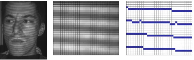
This paper extends the authors’ work described in [10] by investigating the use of PDE mesh surfaces to the compression and reconstruction of large data files without loss of accuracy in the face recognition methods. The source data model typically uses a connected mesh of vertices with triangular faces, which is the standard data type in many 3D computer generated models, such as Wavefront and Java 3D OBJ, VRML and COLLADA formats [3, 1, 7]. In our 3D scanning system [13, 2], the model is a constrained version of this mesh, with rows and columns of vertices connected in a rectangular pattern as depicted in Figure 1, conforming to the stripes in our original projected pattern. The figure clearly shows that in mapping to 3D space we can simply save the 3-part vector for each vertex, without the need for a separate list of faces and vertex connections, as it is required in the 3D file formats mentioned above. This explicit connectivity of the mesh makes interpolations a simpler and more reliable process than with an arbitrarily connected mesh, and gives a more compact data representation, and smaller file size (compared with OBJ, VRML and COLLADA formats).

As an alternative to the compression using polynomials we now intend to create PDE meshes with high vertex density and comparing the compression efficiency of the resulting data with the original data. Within the security theme, in this work we use face models from the 3D scanner, and firstly construct a mesh with high vertex density, we call this the “superfine mesh”. A high density mesh is necessary in order to measure Euclidean distances on the face more accurately to produce the required accuracy and robustness in the face recognition algorithms[8, 11]. It is clearly also important to ensure when this PDE data is reconstructed as the superfine mesh, and used in the face recognition process, there is no loss of accuracy in the reconstructed mesh. Therefore two questions can be posed:

(1) what compression rates can we obtain using the PDE method, and

(2) how can we compare the accuracy the reconstructed PDE, compared with the original superfine mesh?

Section 2 describes the compression and reconstruction method, Section 3 presents ex-perimental results and Section 4 assesses the quality of the reconstructed mesh. Finally, a discussion and conclusions are presented in Section 5.

2. Method

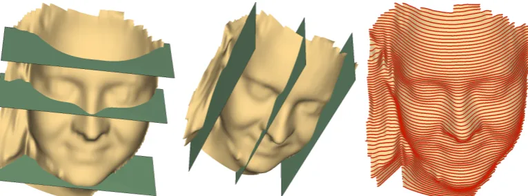
2.1. Data Preparation. The procedure can be described as follows. Given a (poten-tially dense) generic surface patch defined as a single-valued function, the first step is to perform a structured re-meshing aiming a reducing the vertex density [10]. This is achieved by finding the minimum bounding box in 3D [5] and using a number of hori-zontal and vertical cutting planes for vertex sampling. Each plane intersection defines a line, and where this line intercepts the mesh defines a sampled vertex in the plane. All points lying in the plane – either horizontal or vertical – can be treated as a one-dimensional signal and subject to compression. The result of this procedure is that the mesh is redefined as aligned vertices in the horizontal and vertical directions as depicted in Figure 2, where only a few planes are shown for clarity.

It is important to stress here that such re-meshing operation will yield a sparse mesh as it reduces the number of vertices in the original structure. Upon compression by the Fourier technique described below, it only becomes possible to reconstruct the sparse mesh. However, our objective is to recover the vertex density of the original mesh, that’s where the PDE technique comes into play.

The number of required horizontal and vertical cutting planes depends on the mesh complexity. Defining D1 as the distance between structured vertices in the horizontal plane with normal vector (0,1,0)T andD2 between planes with normal vector (1,0,0)T, the (x, y) coordinates of any sampled vertex can be recovered for all planesk:

xr = {rD1,|r= 1,2, . . . , k1} (1)

yc = {cD2,|c= 1,2, . . . , k2} (2)

z = {zi, |i= 1,2, . . . , k1k2} (3)

where (r, c) are the indices of the planes. This is significant as 2/3 of the 3D data can safely be discarded in a sense that it is not necessary to save the actual values (x, y) of each vertex; instead, only the global parameters D1, D2, k1, k2 are kept allowing full reconstruction of (x, y) values in each plane. With this information at hand, from now on we are only concerned with modelling and compressing thez-values.

2.2. Fourier Series. Once the data are in the format specified in Section 2.1, the vertices lying in each plane can be considered as a one-dimensional signal and treated as a Fourier series. The usefulness of the Fourier analysis is that we can break up any arbitrary periodic function into a set of simple terms that can be solved individually and then recombined to reconstruct the original signal to a high degree of accuracy [4]. Using the method of generalized Fourier series, the Fourier series of a function f(x) is given by

(4) f(x) = 1 2a0+

∞ X

n=1

ancos

2πnx

l

+bnsin

2πnx

l

where

a0 = 2

l

Z l

0

f(x)dx

(5)

an =

2

l

Z l

0

f(x) cos 2πnx l dx (6)

bn =

2

l

Z l

0

f(x) sin 2πnx l dx (7) Thus, (8) 1 2a 2 0+ ∞ X n=1

a2_n+b2_n = 1

l

Z l

0

(f(x))2dx.

the coefficients together with the boundaries of each function and their scale it is then possible to reconstruct faithfully the original data defined by the Fourier series. From Equation (4) the experimental data are represented as follows:

(9) y=a0+ancos(nπx) +bnsin(nπx) +a6cos(nπx)

where n is a vector [1,2, ..., N] and N is the length of vector an. Given a signal s of

lengthm, the relevant coefficients in Equation (9) can be evaluated (e.g. using Matlab built-in functions) as:

d = fft(s) (10)

M = floor((m+ 1)/2) (11)

a0 = d(1)m (12)

a6 = d(M+1)/m (13)

bn = −2∗imag(d(2...M))/m. (14)

The set of Fourier coefficients are estimated for each plane and saved in plain ASCII format onto a file with N lines of text where the first line contains header information followed by (N −1) lines of data as defined in Table 1 where:

Table 1. Text file format for 3D compression using DFT

ineLine number ASCII data info ine 1 k1 k2 D1 D2 Q

2 v1 v2 a0 a6 L an bn

. . . .

N v1 v2 a0 a6 L an bn

ine

1 line 1 contains header info, 2 –N lines 2 toN contain data,

k1,k2 are the scale factors or distance between two consecutive horizontal and two consecutive vertical planes in mm,

D1,D2 are the dimensions of the data in number of rows and columns,

v1,v2 are the first and last valid vertices for each row of data,

Q the quality of the compression in percentage from 1 to 100,

a0,a6 are the scalar Fourier coefficients for each row of data,

L the vector length of Fourier coefficients,

an,bn the vector real and imaginary Fourier coefficients for each row of data.

The parameter Q is defined as the quality of the compression and is expressed in per-centage.

2.3. PDE Modelling. We use the Laplace equation [6, 18] of the form:

(15) ∂

2_u

∂x2 +

where x and y are spatial independent variables in Cartesian coordinates. Note that with no derivatives in t, Laplace’s equation require no initial conditions, Because the potential does not depend on time, no initial condition is required. Hence, we are faced with solving a pure boundary value problem.

We discretise the solution onto a rectangular domain (m+ 1) by (n+ 1), with the boundary conditions of the form

u(x,0) =F(x), u(x, b) =G(x), 0< x < a,

(16)

u(0, y) =P(y), u(a, y) =Q(y), 0< y < b.

(17)

where the first and last row of the domain are the experimental data (thez-values of each two consecutive cutting planes) and the problem then is to solve the Laplace equation over the domain. This will insert vertices between the two planes recovering the original mesh density. The series solution can be represented as

(18) u(x, y) = ∞ X

n=1

fnan(a, y) +gnan(x, b−y) +pnbn(x, y) +qnbn(a−x, y)

where

an(x, y) = sin

nπx

a

sinhnπ(b−y)

a

/sinhnπb

a

,

(19)

bn(x, y) = sin

nπ(a−x)

b

sinhnπy

b

/sinhnπa

b

,

(20)

and the constantsfn, gn, pn, andqn are coefficients in the Fourier sine expansions of the

boundary value functions. This implies that

F(x) = ∞ X

n=1

fnsin

nπx

a

, G(x) = ∞ X

n=1

gnsin

nπx

a

,

(21)

P(y) = ∞ X

n=1

pnsin

nπy

b

, Q(y) = ∞ X

n=1

qnsin

nπy

b

(22)

The coefficients in the series can be computed by integration or approximate coefficients can be obtained using the FFT as described in Section 2.2.

Here we can have either Dirichlet, von Neumann or mixed boundary conditions to specify the four boundary conditions of the rectangular domain. If the value of the solution is given around the boundary of the region, then the boundary value problem is called a Dirichlet problem, whereas if the normal derivative of the solution is given around the boundary, the problem is known as a von Neumann problem. In the experimental results described below we use Dirichlet boundary conditions by fixing the value of the vertices in the boundaries of the rectangular domain.

3. Experimental Results

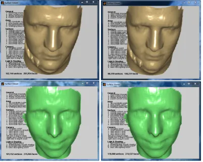
Figure 3. Left: original meshes; right: PDE reconstructed

The processing of the above data and the 3D reconstruction involves solving the PDE as described in Section 2.3 between two consecutive cutting planes π1 and π2. The proposed PDE methodology is highlighted as follows. Each plane contains a number of vertices, some are valid while some are invalid. Only the valid vertices from one plane are paired to their valid counterparts with the same index in the other plane. The PDE surface is then defined by solving the Laplace equation between each pair of cutting planes. Thus, the PDE boundary conditions are set between the two planes; the

x variable in the PDE defines the number of vertices we wish to interpolate between any two planes, and the number of iterations is set to 10 for all planes. For instance, a PDE surface with 5 steps in x means that we are generating 3 extra vertices between the original pair of vertices.

this resulted into 72 horizontal planes on each mesh and 563 vertical planes. Fourier coefficients were estimated for the z-values of each of the 72 planes and saved into the prescribed format. These operations reduced the file size from 20 MB down to 668KB, a reduction of over 96.6% (if the file were zipped then the final size would only be 111KB, a reduction of over 99.4%). The pictures on the right column show the reconstructed meshes using the PDE method as described above. Due to the Nyquist sampling theorem the reconstructed meshes are half the size of the original mesh, i.e. the number of vertices along each cutting plane is half their original numbers; this is shown on the mesh on top right of Figure 3. On the bottom right, we added vertices by averaging every two neighbouring vertices. It can be clearly seen that PDE reconstruction from compressed files as defined in this paper does preserve the quality of the mesh.

4. Assessing the Quality of 3D Reconstruction

Determining the goodness of fit or how well the 3D reconstructed data points fit the original data can involve a number of tests including statistics summaries. Here we perform an assessment in a number of different ways: (1) visual assessment of the data and residuals, (2) residuals plotted against predicted values, (3) a normal-probability plot of the residuals, and (4) the coefficient of determinationR2.

By far the most meaningful way is by plotting the original and reconstructed data sets and visually assess their quality as depicted in the examples of Figure 3. Visual inspection suggest that there is a perceived good fit between the PDE reconstructed data and the original data sets. However, quantitative data would allow us to objectively compare the goodness of fit. By subtracting the PDE reconstructed from the original mesh, we would expect that, if the two meshes were exactly the same, then the difference would describe a zero-plane at origin with normal (0,0,1)T, as all vertex differences would be zero. Figure 4 left shows such a difference surface with vertex values oscillating around zero. Although there are small errors across the surface especially around the nose area and at the boundaries of the mesh, such errors may not be significant enough to impair recognition algorithms. On the right of Figure 4 it is shown a quantification of the error surface – essentially a view of the residuals across the yz-plane. Note that the nose region is at the centre of the plot while the left and right regions of the plot correspond to the oscillations observed in the error surface. The majority of the errors are within range±1mm with the largest error approaching 2.5mm at the boundaries.

Another way of assessing the quality of the reconstructed mesh is to look at the residuals and plot them against their predicted values. Figure 5 left depicts a scatter plot of reconstructed against original data. For a good fit, the plot should display no patterns and no trends, and this is verified in the plot indicating a good measure of fit. Similarly, a normal-probability plot of the residuals should display a straight line for a good fit. On the right of Figure 5 it can be verified that most data sets evaluated at each plane are in straight lines, indicating a good fit.

Figure 4. On the left, a visualisation of the error surface and, on the right the quantification of such errors in mm.

Figure 5. Left: Scatter plot of Predicted Values against Residuals (a good fit is indicated by no patterns and no trends). Right, The normal-probability plot of the residuals (a good fit is indicated by a straight line for each set of data)

variation in the data explained by the model is given byR2 = 1−(SSE)/(SST) expressed as percentage. The R2 values for the PDE interpolated data are above 0.98 for all data sets described in this paper. Again this indicates a good measure of fit and suggests that the method is appropriate to a variety of applications.

5. Discussion and Conclusions

Fourier analysis of data in each plane is performed and the Fourier coefficients together with scale information are saved onto an ASCII file in a prescribed format. The file is then read and each plane is reconstructed using the Fourier coefficients recovering the sampled, sparse mesh. The high density mesh is obtained comparable to the original mesh by solving the PDE mesh between each pair of cutting planes through the Laplace equation.

Evaluating the success of these methods will depend on the applications in which they are used; we make the assumption that the surfaces are fairly complex with concave and convex local features. The face is such a case, and in Figure 4 left we see some errors around the nostrils and, to a lesser extent, the sides of the nose in our experimental data. In our face recognition application, because the nostrils are a known cause of errors, we avoid making measurements in this area, so the results in our new model will not cause significant problems. In the experiments described here, the source of some errors are due to rounding off values of the Fourier coefficientsan and bn. Rounding increases the

efficiency of data compression: for each entry in those vectors if abs(an, bn)<0.001 the

values are rounded to zero. The percentage of rounded coefficients defines the quality parameter; e.g. for quality=100, no rounding off is applied.

Experimental results have demonstrated that the method is highly efficient and allows high quality full reconstruction of the original mesh. The PDE-based method allows the recovery of the original mesh that has been compressed by over 96%. Both visual analysis and statistical measures demonstrate the effectiveness of the method. Error surfaces are relatively small and while it is accepted that the quality of the reconstructed data depends on the characteristics of the original data, results indicate the generality of the method for 3D data compression.

The method presented here is feasible for the airport scenario discussed in Section 1 and, because all compressed data (represented by the Fourier coefficients) are saved onto relatively small plain text files, it would be amenable to fast and secure encryption algorithms. This means that all 3D data can be efficiently and securely transmitted over a network. Future work will be focussed on defining optimal PDE parameters aiming at reducing error surfaces and perform sensitivity analysis concerning levels of noise, smoothness of the surface, rounding off errors and complexity of each cutting plane.

References

[1] Ames, A.L., D.R. Nadeau, J.L. Moreland (1996). VRML 2.0 2E W/CD, John Wiley & Sons; 2nd Edition, 654pp.

[2] Brink, W., A. Robinson, and M. Rodrigues (2008). Indexing Uncoded Stripe Patterns in Structured Light Systems by Maximum Spanning Trees,British Machine Vision Conference BMVC 2008, Leeds, UK, 1–4 Sep 2008.

[3] Chen, J.X. and C. Chen (2008). Foundations of 3D Graphics Programming: Using JOGL and Java3D, Springer, 400pp.

[4] Hanna, J.R. and J.H. Rowland (2008). Fourier Series, Transforms, and Boundary Value Problems, Dover Books on Mathematics.

[5] Hill, F.S. Jr (2001). Computer Graphics Using OpenGL, 2nd edition, Prentice-Hall Inc, 922pp.

[6] Nirenberg, L. (1972). Lectures on linear partial differential equations, American Mathe-matical Society,1972.

[8] Rodrigues, M.A. and A. Robinson (2011). Real-time 3D Face Recognition using Line Projec-tion and Mesh Sampling. In: EG 3DOR 2011 - Eurographics 2011 Workshop on 3D Object Retrieval, Llandudno, UK, 10th April 2011. Eurographics Association. p9–16.

[9] Rodrigues, M.A. and A. Robinson (2011). Fast 3D recognition for forensics and counter-terrorism applications. In: AKHGAR, Babak and YATES, Simeon, (eds.) Intelligence man-agement : knowledge driven frameworks for combating terrorism and organized crime. Ad-vanced information and knowledge processing . London, Springer-Verlag, 95-109.

[10] Rodrigues, M.A., A.Osman and A. Robinson (2010). Efficient 3D Data Compression Through Parameterization of Free-Form Surface Patches, 2010 International Conference on Signal Processing and Multimedia Applications (SIGMAP), 26-28 July 2010, p130–135. [11] Rodrigues, M.A. and A. Robinson (2010). Novel methods for real-time 3D facial recognition.

In: SARRAFZADEH, Majid and PETRATOS, Panagiotis, (eds.) Strategic Advantage of Computing Information Systems in Enterprise Management. Athens, Greece, ATINER, 169-180.

[12] Rodrigues, M.A., A. Robinson, and W. Brink (2008). Fast 3D Reconstruction and Recog-nition, inNew Aspects of Signal Processing, Computational Geometry and Artificial Vision, 8th WSEAS ISCGAV, Rhodes, 2008, p15–21.

[13] Robinson, A., L. Alboul and M.A. Rodrigues (2004). Methods for Indexing Stripes in Un-coded Structured Light Scanning Systems,Journal of WSCG, 12(3), 2004, pp 371–378. [14] Schiesser, W.E. and G.W. Griffiths (2009). A Compendium of Partial Differential

Equa-tion Models: Method of Lines Analysis with Matlab, ISBN-13 978-0-521-51986-1, Cambridge University Press, Cambridge, UK.

[15] Szymczak, A., D. King and J. Rossignac (2000). An Edgebreaker-Based Efficient Compres-sion Scheme for Regular Meshes, 12th Canadian Conference on Computational Geometry, pp 257–265.

[16] Szymczak, A., J. Rossignac, and D. King (2002), Piecewise Regular Meshes, Graphical Models 64(3-4), 2002, 183–198.

[17] Shikhare, D., S.V. Babji, and S.P. Mudur (2002). Compression techniques for distributed use of 3D data: an emerging media type on the internet, 15th international conference on Computer communication, India, pp 676–696.