Propagation of coronal mass ejections in the inner heliosphere

(1)

Propagation of Coronal Mass Ejections in

the Inner Heliosphere

Shane A. Maloney, B.Sc. (Hons.)

School of Physics

Trinity College Dublin

A thesis submitted for the degree of

PhilosophiæDoctor (PhD)

September 2011

(2)

(3)

Declaration

I declare that this thesis has not been submitted as an exercise for a degree at this or any other university and it is entirely my own work.

I agree to deposit this thesis in the University’s open access institutional repos-itory or allow the library to do so on my behalf, subject to Irish Copyright Legislation and Trinity College Library conditions of use and acknowledgement.

(4)

Summary

Solar Coronal mass ejections (CMEs) are large-scale ejections of plasma and magnetic field from the corona, which propagate through interplanetary space. CMEs are the most significant drivers of adverse space weather on Earth, but the physics governing their propagation through the Heliosphere is not well understood. This is mainly due to the limited fields-of-view and plane-of-sky projected nature of previous observations. The Solar Terrestrial Relations Ob-servatory (STEREO) mission launched in October 2006, was designed to over-come these limitations.

In this thesis, a method for the full three dimensional (3D) reconstruction of the trajectories of CMEs using STEREO was developed. Observations of CMEs close to the Sun (<15R) were used to derive the CMEs trajectories in 3D. These reconstructions supported a pseudo-radial propagation model. Assuming pseudo-radial propagation, the CME trajectories were extrapolated to large distances from the Sun (15 – 240R). It was found that CMEs slower than the solar wind were accelerated, while CMEs faster than the solar wind were decelerated, with both tending to the solar wind velocity.

(5)

near Earth was determined.

CMEs are known to generate bow shocks as they propagate through the corona and SW. Although CME-driven shocks have previously been detected indirectly via their emission at radio frequencies, direct imaging has remained elusive due to their low contrast at optical wavelengths. Using STEREO observations, the first images of a CME-driven shock as it propagates through interplanetary space from 8Rto 120R(0.5 AU) were captured. The CME was measured to have a velocity of_∼1000 km s−1_{and a Mach number of 4}_.₁_±₁_._{2, while the shock}

front standoff distance (∆) was found to increase linearly to _∼20R at 0.5 AU. The normalised standoff distance (∆/DO) showed reasonable agreement

with semi-empirical relations, where DO is the CME radius. However, when

normalised using the radius of curvature (∆/RO), the standoff distance did not

agree well with theory, implying that RO was underestimated by a factor of

(6)

To my parents,

(7)

Acknowledgements

I am extremely grateful to my supervisor Peter Gallagher, whose experience, advice, and enthusiasm has been vital on many occasions. It has been a pleasure working with you these past four years.

I must also thank James McAteer and Shaun Bloomfield whose guidance and discussions have been most helpful.

I must also express my appreciation to all the staff in the School of Physics without your efforts the school would grind to a halt.

During my times at Goddard a huge thank you must go to Alex, Jack and Dominic. Whether it was helping to sort out my financial situation, or ideas and thoughts on my research or outside of work, you helped make my time at Goddard all that is was.

A huge thank you also goes out to my fellow comrades in arms in the office, past and present; Aidan, Claire, David, Eoin, Eamon, Joseph, Jason, Larisza, Paul C, Paul H, Peter, Sophie. Whether it was discussing the finer points of IDL, general banter in the office, morning coffee, or after work pints you have made my time here more enjoyable then I imagined it could be. My gratitude also goes to all the guys from ACTTT and BOXMASTERS who kept me from leading a completely sedentary lifestyle.

(8)

(9)

List of Publications

1. Gallagher, P. T.,Maloney, S. A. et al.

“A comprehensive overview of the 2011 June 7 event”, Astronomy & Astrophysics,in prep

2. P´erez-Su´arez, D.,Maloney, S A., Higgins, P. A. et al.

“Studying Sun-planet connections using the Heliophysics Integrated Observatory (HELIO)” Solar Physicsin review

3. Maloney, S. A.and Gallagher, P. T.

“STEREO Direct imaging of a coronal mass ejection driven shock to 0.5 AU”, Astrophysical Journal Letters, 736, L5, 2011

4. Byrne, J. P.,Maloney, S. A., McAteer, R. T. J., Refojo, J. M. and Gallagher, P. T. “Propagation of an Earth-directed coronal mass ejection in three dimension”, Nature Communications, 1, 74, 2010

5. Mierla, M.,Maloney, S. A. et al.

“On the 3-D reconstruction of Coronal Mass Ejections using coronagraph data”, Annales Geophysicae, 28, 203, 2010

6. Maloney, S. A.and Gallagher, P. T.

“Solar Wind Drag and the Kinematics of Interplanetary Coronal Mass Ejections”, Astrophysical Journal Letters, 724, L127, 2010

7. Maloney, S. A., Gallagher, P. T. & McAteer, R. T. J.

“Reconstructing the 3-D trajectories of CMEs in the inner Heliosphere”, Solar Physics, 256, 149, 2009

(14)

0. LIST OF PUBLICATIONS

(15)

List of Figures

1.1 Structure of the Sun . . . 4

1.2 Sound Speed in the Interior of the Sun . . . 6

1.3 αΩ-Dynamo . . . 7

1.4 Butterfly Diagram . . . 9

1.5 Temperature and Electron Density in the Solar Atmosphere . . . 10

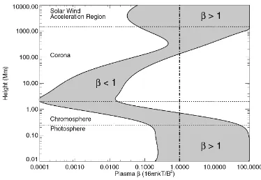
1.6 Plasma-β in the Solar Atmosphere . . . 11

1.7 Parker’s Solar Wind Solutions . . . 17

1.8 Parker Spiral . . . 20

1.9 Solar Wind Speed Measured by Ulysses . . . 21

1.10 The Heliosphere . . . 22

1.11 Typical ‘lightbulb’ CME . . . 23

1.12 Images of Aurora from the ground and ISS . . . 24

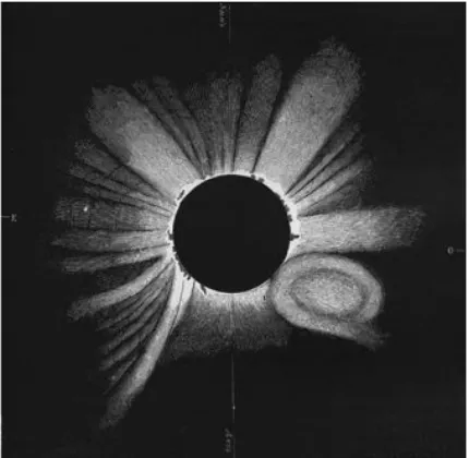
1.13 1860 Eclipse Sketch . . . 26

1.14 Type II and III Radio Burst Height-Time Plot. . . 27

1.15 Gosling’s CME Flare Paradigm . . . 30

1.16 Magnetic Cloudin situMeasurements . . . 31

1.17 Possible Spacecraft track through a CME . . . 32

1.18 CME Velocity Evolution with soft X-ray light Curve . . . 33

1.19 CME Kinematics Fit with double exponential and corresponding soft X-ray Flux . . . 34

1.20 CME Kinematics with corresponding hard X-ray Flux . . . 35

1.21 Polarimetric CME Reconstruction . . . 36

1.22 CME Acceleration far from the Sun . . . 37

1.23 Comparison of CMEs speeds close to the Sun to those at 1 AU . . . 38

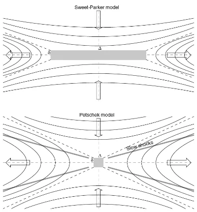
2.1 Sweet-Parker and Petshek Reconnection Geometries . . . 47

(16)

LIST OF FIGURES

2.3 Cartoon Showing Mechanical Analogies for CME Initiation Mechanisms . . 52

2.4 Theoretical Evolution of 2D Flux Rope . . . 55

2.5 3D Flux Rope Model . . . 57

2.6 Toroidial Instability Simulation . . . 58

2.7 3D Toroidal Instability Simulation . . . 59

2.8 3D Potential Magnetic Field Bundle . . . 60

2.9 3D Kink Instability Simulation . . . 62

2.10 Breakout Schematic and Simulation . . . 63

2.11 Breakout CME Simulation . . . 64

2.12 Aerodynamic Drag Simulation . . . 68

2.13 Comparison of Aerodynamic Drag and ‘snow plough’ Models to Observations 69 2.14 Flux Rope CME Propagation Simulation . . . 70

2.15 Imaging Observations of Bow Shocks Formed by a Bullet and Star . . . 71

2.16 Shock Frames of Reference . . . 73

3.1 Thomson Scattering Schematic . . . 79

3.2 Thomson Sphere and Scattered Intensity . . . 81

3.3 Thomson Scattering Effect on Morphology . . . 82

3.4 Basic CME Structure and Observational Interpretations . . . 83

3.5 Plane-of-Sky Projected Kinematic Representative of STEREO . . . 84

3.6 Optical Layout of Lyot Coronagraph . . . 85

3.7 Schematic of the SOHO Spacecraft . . . 88

3.8 Schematic of EIT . . . 88

3.9 Sample EIT 171˚A Observation . . . 89

3.10 Schematic of C2 . . . 90

3.11 Schematic of C3 . . . 92

3.12 Sample LASCO C3 Observation . . . 93

3.13 Schematic of the STEREO B Spacecraft . . . 94

3.14 STEREO Orbit Progression . . . 95

3.15 Schematic of EUVI . . . 96

3.16 Sample EUVI 195˚A Observation . . . 97

3.17 Schematic of COR1 . . . 98

3.18 Schematic of COR2 . . . 99

3.19 Sample COR2 Observation . . . 100

3.20 HI Concept and Cross-section . . . 102

(17)

LIST OF FIGURES

3.22 HI fields-of-view and theoretical light rejection Levels . . . 103

3.23 Schematic of HI1 and HI2 Optics . . . 104

3.24 Sample HI1 Observation . . . 105

3.25 CME Progression through HI1 and HI2 Fields-of-view . . . 106

3.26 Projection Geometries . . . 108

3.27 Stonyhurst Coordinates . . . 110

3.28 Heliocentric Coordinates . . . 111

4.1 COR1 Image Processing . . . 118

4.2 COR2 Image Processing . . . 119

4.3 HI1 Image Processing . . . 121

4.4 HI2 Image Processing . . . 122

4.5 Epipolar Geometery . . . 123

4.6 3D Reconstruction Geometry . . . 124

4.7 Tie-Point of a Curved 3D Surface . . . 131

4.8 Elliptical Tie-Pointing . . . 132

4.9 CME Drag Simulation . . . 133

5.1 Kinematics Derived form various Methods from Synthetic SECCHI Obser-vations . . . 137

5.2 Sample Observations from the 2007 October 08–13 Event . . . 139

5.3 Sample Observations from the 2008 March 25-28 Event . . . 140

5.4 Sample Observations from the 2008 April 09–10 Event . . . 141

5.5 Sample Observations form the 2008 April 09-13 Event . . . 142

5.6 3D Trajectory Error Analysis . . . 144

5.7 STEREO 3D CME Height and LASCO CDAW De-projected Height . . . . 145

5.8 3D CME Trajectory for 2007 October 08–13 Event . . . 146

5.9 3D CME Trajectory for 2008 March 25–27 Event . . . 147

5.10 3D CME Trajectory for 2008 April 09–10 Event . . . 148

5.11 3D CME Trajectory for 2008 April 09–13 Event . . . 149

6.1 Simulation of a Flux Rope in a Magnetohydrodynamic Flow . . . 155

6.2 Sample Observations from the 2008 March 25 Event . . . 158

6.3 Composite of STEREO-A and B Images from SECCHI of the CME on 12 December 2008 . . . 159

6.4 Derived Kinematics for the 2007 October 8 Event . . . 162

(18)

LIST OF FIGURES

6.6 Derived Kinematics of the 2008 April 09 Event . . . 164

6.7 Derived Kinematics of the 2008 December 12 Event . . . 166

6.8 Bootstrap Distributions for the 2008 December 12 Event . . . 168

7.1 CME and Shock Diagram . . . 172

7.2 CME and Shock Observations . . . 175

7.3 Projection of the 3D Reconstructions of CME and Shock as well as Shock Front Fitting . . . 177

7.4 Plot of the Shock Stand-Off Distance against CME Height . . . 179

7.5 Plot of Derived Shock Properties . . . 180

7.6 Comparison of Normalised Standoff Distance to Models . . . 182

8.1 xImager Software Screen Shot . . . 189

8.2 Corongraph Images Filtered Using an Isotopic Wavelet and Curvelet . . . . 195

8.3 Curvelet Decomposition of a HI1 Image . . . 196

8.4 CME Detection using Thresholding and Morphological Operators . . . 197

8.5 Synthetic Graduated Cylindrical Shell STEREO Observations . . . 198

8.6 ENLIL Simulation Results . . . 199

(19)

List of Tables

3.1 Summary of Instruments . . . 86 6.1 Summary of Fit Parameters . . . 165

(20)

LIST OF TABLES

(21)

Chapter 1 Introduction

In this chapter I will introduce the fundamental physics and concepts that are discussed in this thesis, beginning with a short introduction to the Sun, its various layers, atmosphere,

and activity. This is followed by an introduction to coronal mass ejections (CMEs) which

consists of a historical account of CME observations and their interpretation and a brief review of the modern perspective on CMEs. Finally, I discuss some of the open questions

surrounding CMEs.

(22)

1. INTRODUCTION

“Physicists say we are made of stardust. Intergalactic debris and far-flung atoms, shards of carbon nanomatter rounded up by gravity to circle the sun. As atoms pass through an eternal revolving door of possible form, energy and mass dance in fluid relationship. We are stardust, we are man, we are thought. We are story.”

Glenda Burgess (The Geography of Love: A Memoir)

Since the dawn of mankind the Sun has been a source of great wonder and fascination. Some early civilisation worshipped the Sun as deity, indeed some of our oldest antiqui-ties such as Newgrange and Stonehenge are believed to be solar observatories of a form. Building these monuments required detailed knowledge of the Sun’s motion relative to the Earth, and ever since then we have been increasing our knowledge of the Sun. As science and technology advanced we began to probe the Sun’s structure, composition and energy source. This led to a picture of the Sun, in terms of stellar equations, as a hot ball of gas in equilibrium, with gravitational contraction being balanced by the energy released during nuclear fusion. The modern era of space borne observations has revealed the dynamic and active nature of the Sun in the form of sunspots, filaments, prominences, flares and coronal mass ejections (CMEs). The Sun is the power source for all life on Earth and will also ultimately be the cause of its death.

1.1 The Sun

The Sun, our nearest star, is a main sequence star of spectral type G2V. The Sun has a total luminosityL= (3.84±0.04)×1026W, mass M= (1.9889±0.0003)×1030kg and a radiusR= (6.959_±0.007)_×108_{m (Foukal, 2004). As all stars, the Sun was born from}

a giant molecular cloud of approximate mass 104₋106Mwhich began to gravitationally collapse and fragment. The process of collapse and fragmentation continued until one of these fragments attained a central temperature large enough to start hydrogen fusion, about 4.6_×109 years ago (Prialnik, 2009). At this point fusion taking place in the core produced enough energy to counterbalance the gravitational collapse. Currently the Sun is in a stable configuration, on the Main Sequence, where it is in hydrostatic equilibrium (_∇P =₋ρg). The Sun will continue to maintain this stable state for about another 5_×109 years before entering the red giant phase. At this point the Sun will expand to about 100 times its current size and begin shedding its outer layers, due to successive nuclear burning in ever more distant shells. This ultimately leads to the total loss of the outer envelope exposing a degenerate core, in which all nuclear burning has ceased, called a white dwarf (Phillips, 1995).

(23)

1.1 The Sun

1.1.1 Solar Interior

The modern picture of the Sun’s interior structure has been built up over time, the three most important contributions to this have been the ‘standard solar model’ (SSM; Bahcall

et al. 1982), helioseismology, and solar neutrino observations. As we cannot directly

ob-serve the interior of the Sun we have to model its structure and then compare the model to observed properties, iteratively changing the model parameters until they match the observations. The SSM is essentially several differential equations derived from fundamen-tal physics principles, which are constrained by boundary conditions (mass, radius, and luminosity). The SSM treats the Sun as a spherically symmetric, quasi-static system which is powered by nuclear reactions at its hottest part, the core. The system is assumed to start out as a cloud of primordial gas which collapses under gravity. The composition of this cloud and hence the Sun can only be altered by the process of ‘nuclear burning’ in the core. All the energy generated by the nuclear burning is transported by radiation except where convection is a more efficient process.

The process of ‘nuclear burning’ or nuclear fusion occurring in the core at about 1.5_× 107K, is the power source of the Sun. The proton-proton (p-p) chain describes the basic process which occurs:

1

1H +11H→21H +e++νe (1.1)

2

1H +11H→32He +γ (1.2)

3

2He +32He→42He + 211H (1.3)

where1₁H is hydrogen, 2₁H is an isotope of hydrogen (deuterium), 4₂He is helium, 3₂He is an isotope of helium with one neutron,e+_{a positron,}_ν

e an electron neutrino andγ a photon.

The p-p chain splits off into three branches at (1.2) which operate simultaneously, their reaction rates are determined by the density, temperature, and elemental abundances in the core. The net result of the p-p chain is the fusion of 4 hydrogen nuclei to from a Helium nuclei or α-particle:

41₁H→42He (1.4)

with the products weighing less than sum of the initial masses by 0.02866 amu or 4.8_× 10−29kg. Using Einstein’s mass energy relationE =mc2 this results in a energy output of 4.28_×10−12_{J (26.73 MeV) of which varyingly small proportions are carried away by the}

neutrinos (Foukal, 2004; Phillips, 1995). Comparing the total energy output of the Sun (L) to the energy released during one cycle of the p-p chain we can estimate the reaction rate to be 8.97_×1037_s−1_{. The region where the temperatures and densities are high enough}

(24)

[image:24.612.107.464.171.524.2]

1. INTRODUCTION

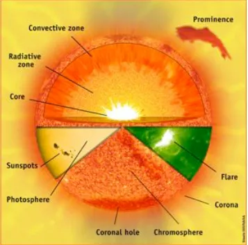
Figure 1.1: At the centre of the Sun is the core (_≤0.25R) where temperatures reach

∼1.5_×107_{K, high enough for fusion to take place. The energy generated at the core from}

the fusion process is transported towards surface via thermal radiation in the radiative zone (0.25 – 0.70R). At this point the solar plasma is cool enough to from highly ionised atoms

and becomes optically thick. As a result it is convectively unstable and energy is transported through mass motions in the convection zone (0.7 – 1.0R). The visible surface of the Sun, the

photosphere, is a thin layer in the atmosphere where the bulk of the Sun’s energy is radiated, its spectra is well matched to a blackbody with peak temperature of 5,600 K. Above the Sun’s visible surface lies the chromosphere and finally the corona where the temperature soars back up to 1 – 2×106_{K. Image courtesy of Steele Hill NASA/GSFC.}

(25)

1.1 The Sun

for fusion to occur is known as the core, and extends out to about 0.25R (Figure 1.1). Outside of the core is the radiative zone (0.25 – 0.70R) where thermal radiation is the most efficient means of transporting the intense energy generated in the core, in the form of high energy photons, outward. The temperature drops from about 7_×106K at the bottom of the radiative zone to 2×106K just below the convection zone. As the radiation is thermal it is described by the Planck (blackbody) equation, the specific radiative intensity is given by:

Bλ(T) =

2hc2

λ5

1 exp_λkhc

BT

−1

W m2_{sr m}

(1.5)

where h is the Planck constant, cis the speed of light, k is the Boltzmann constant. The peak of this function is given by Wein’s displacement law λmax = 2.8977×10−3T−1m K

thus the radiative zone is dominated by x-ray and gamma-ray photons. Due to the still high densities (2×104– 2×102kg m−2) in the radiative zone the mean free path of the photons is very small (_∼9.0_×10−2_{cm) hence it can take tens to hundreds of thousands}

of years to escape (Mitalas & Sills, 1992). As the temperature continues to fall, highly ionised atoms begin to form once an appreciable number of atoms have formed the plasma becomes optically thick, and as a result, becomes unstable as indicated by the upper limit of the Eddington luminosity:

κF <4πc Gm (1.6)

where κ is the opacity, F the radiation flux, Gthe gravitational constant, c the speed of light and m the mass coordinate (Prialnik, 2009). The sudden increase in opacity above the radiative zone causes the plasma to become convectively unstable. In this region called the convection zone (0.7–1.0R), convection is the dominant form of energy transport. If the mass motions are rapid enough to assume they are adiabatic, and radiation pressure negligible, the Schwarzchild criterion for stability against convection may be used:

dT dr star =

γ₋1

γ dP dr star (1.7)

whereγ =CP/CV is the ration of specific heats (Prialnik, 2009). This gives a lower limit

on the conditions necessary for convection to occur. In other words for convection to occur the temperature gradient must be larger than the adiabatic gradient.

Helioseismology allows us to probe the solar interior by studying the propagation of sound waves in the Sun. Solar pressure waves (p-modes) are believed to be generated by the turbulence in the convection zone near the surface of the sun. Only certain allowed modes (spherical harmonics) can persist, as a result the Sun ‘rings’ like a bell. As these acoustic

(26)

[image:26.612.83.412.168.408.2]

1. INTRODUCTION

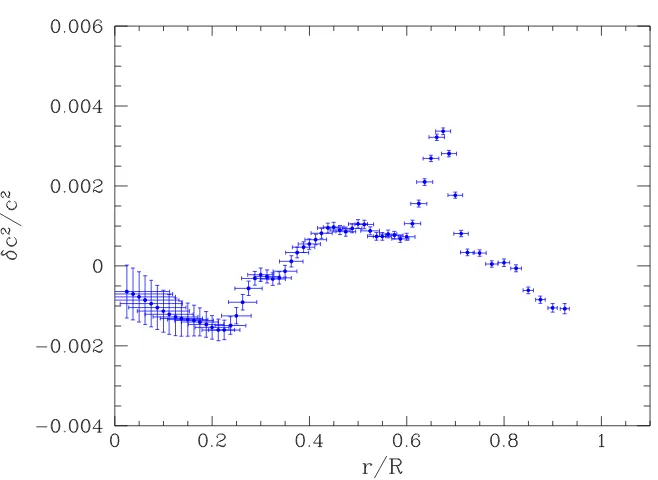
Figure 1.2: This plot shows the relative differences between the squared sound speed in the Sun inferred from two months of Michelson Doppler Imager (MDI) data and from the SSM. The feature at about 0.7 r/R corresponds to the tachocline. The horizontal bars show the spatial resolution, and the vertical bars are the error estimates. Image courtesy of Stanford Solar Oscillations Investigation (SOI).

waves travel, they are refracted due to the waves’ speed dependance on temperature, hence depth. This means that for all allowed modes the waves will be propagating normal to the solar surface when they reach it. This motion of the wave can be detected as Doppler shifts at the surface. Different modes penetrate to different depths and by combining a large number, the entire solar interior can be studied. The comparison of the properties derived from helioseismology, and that of the SSM can be used to change the model parameters to better fit the data, and the modern comparisons are extremely good as shown in Figure 1.2 During the fusion process a large number of neutrinos are produced and escape the Sun. These neutrinos can be detected on Earth and the flux compared to predictions from the SSM. When this was first done for the rare 8B neutrino flux (p-p III chain; Prialnik, 2009), there was a large discrepancy between the predicted flux and the observed

(27)

1.1 The Sun

Figure 1.3: Left: Shows the Sun’s bipolar field. Middle: The magnetic field is being twisted by differential rotation. Right: Loops of magnetic field begin to break the surface forming sunspots. (From The Essential Cosmic Perspective, by Bennett et al)

flux, which was only _∼ 0.4 of the predicted value and led to the so-called ‘solar neutrino problem’ (Bahcall, 2003). Results from helioseismology strongly suggested that the SSM was correct, but the experimental neutrino results were rigorously tested and found to be correct, leaving a serious issue with either the standard model for particle physics, or with the SSM. The problem was resolved when it was theorised that neutrinos could oscillate, that is an electron neutrino (νe) could become a muon neutrino (νµ) as it propagated

from the Sun to the Earth. This was a large step as it required the neutrino to have a small but finite mass. It became clear that the early experiment to measure the neutrino flux was only sensitive to electron neutrino (νe) and so could have ‘missed’ some of the

flux. Today the 8_{B measured neutrino flux (from the 3 flavours, electron, muon, and}

tau) is (5.44±0.99)×106neutrinos/cm2s in good agreement with the SSM prediction of (5.05₋+1₀_..0₈)×106neutrinos/cm2s (Bahcall, 2003).

The core and the radiative zones of the Sun rotate rigidly (as a solid body) but the convection zone rotates differentially, there is a thin interface between the two regions known as the tachocline. Due to the meeting of the two bodies rotating at different rates

(28)

1. INTRODUCTION

this region is subjected to large shear flows. These flows are believed to be the mechanism that generates the Sun’s large-scale magnetic field and powers the solar dynamo. The Sun’s magnetic field is mainly dipolar and aligned to the rotation axis, thus each hemisphere has an opposite dominant polarity (Figure 1.3 left). The differential rotation of the convection zone winds-up this field. This large scale twisting which transforms poloidal field to toroidal field is know as the Ω-effect (Figure 1.3 middle). As the field is twisted up the magnetic pressure increases and bundles of magnetic field lines (flux ropes) can become unstable and rise up in the from of loops. Due to solar rotation, the Coriolis effect twists these loop back towards north-south orientation reinforcing the original poloidal field, this is known as the

α-effect (Figure 1.3 right) and completes the αΩ-dynamo. When magnetic loops become buoyant and rise up through the surface they are visible as sunspots on-disk and mark the footprints of large loops which extend into the solar atmosphere. In a given hemisphere the leading sunspot and trailing sunspot will have opposite polarities, this order is reversed in the other hemisphere (Hale’s Law). Also the tilt angle of the sunspots pairs have a mean value of 5.6◦relative to the solar equator (Joy’s Law). Sunspots are known to migrate from high latitudes towards the equator over an 11 year cycle (Sporer’s Law; see Figure 1.4). The net affect is an increase in opposite polarity field at the poles, ultimately the majority of the field will be oppositely oriented and the dipole will flip. This occurs every 11 years, thus a complete cycle takes 22 years (N to S to N). The activity of the Sun, in the form of active regions, flares, transient events, and other associated phenomenon, is modulated by this cycle (see Figure 1.4 lower).

1.1.2 Solar Atmosphere

The Sun’s atmosphere is composed of all the regions above the photosphere. Until now we have referred to the photosphere as the visible surface of the Sun, it is in fact a very thin layer of the solar atmosphere. The solar atmosphere is usually separated into three regions, the photosphere, chromosphere and corona based on their density, temperature, and composition as shown in Figure 1.5. However, this separation is a simplification as the atmosphere is an in-homogenous mix of different plasma properties due to up-flows, down-flows, heating, cooling and other dynamic processes. The density of the plasma gen-erally decreases through these regions with increasing height. The temperature decreases, reaching a minimum in the chromosphere, then slowly rises until there is a rapid increase at the transition region which continues into the corona. This rapid increase in temperature leads to the so-called ‘coronal heating problem’.

(29)

1.1 The Sun

1870 1880 1890 1900 1910 1920 1930 1940 1950 1960 1970 1980 1990 2000 2010 DATE

AVERAGE DAILY SUNSPOT AREA (% OF VISIBLE HEMISPHERE)

0.0 0.1 0.2 0.3 0.4 0.5

1870 1880 1890 1900 1910 1920 1930 1940 1950 1960 1970 1980 1990 2000 2010 DATE

SUNSPOT AREA IN EQUAL AREA LATITUDE STRIPS (% OF STRIP AREA) > 0.0%> 0.0% > 0.1%> 0.1% > 1.0%> 1.0%

90S 30S EQ 30N 90N

12 13 14 15 16 17 18 19 20 21 22 23

http://science.nasa.gov/ssl/pad/solar/images/bfly_new.ps NASA/NSSTC/HATHAWAY 2005/10

[image:29.612.133.529.185.412.2]

DAILY SUNSPOT AREA AVERAGED OVER INDIVIDUAL SOLAR ROTATIONS

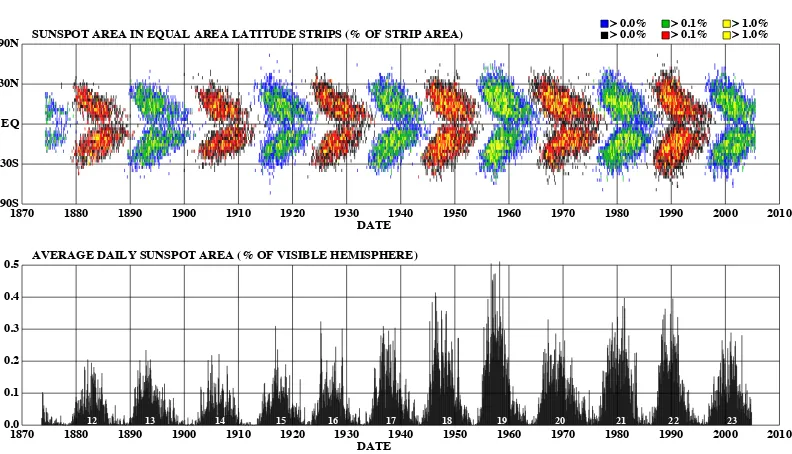
Figure 1.4: The position of the sunspots in equal area latitude strips, averaged over a solar rotation with respect to time (top). The butterfly pattern is clear as the decrease in the upper limit of sunspot latitudes with time. (bottom) The average sunspot area as a function of time. The 11 year modulation is clear in both of these plots. Image courtesy of NASA MSFC.

ratio of the thermal to magnetic pressures:

β = pth

pmg

= nkBT

B2_/₂_µ 0

, (1.8)

where nis the number density and µ0 the permeability of free space. In the photosphere

the plasma-β is large and the plasma motions carry the field with them (Figure 1.6). Ascending into the chromosphere and corona the plasma-β becomes small and the plasma is constrained to follow the magnetic fields. Continuing upwards the plasma-βdrops again and the magnetic field is advected out with the solar wind plasma flow and ultimately forms the Parker spiral (Figure 1.6).

(30)

[image:30.612.118.457.114.354.2]

1. INTRODUCTION

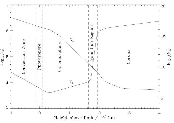
Figure 1.5: A 1D model of the electron density Ne [cm−3] and temperature Te [K] profile thought the solar atmosphere from Gallagher (2000) after Gabriel & Mason (1982). Neutral atoms are present in the photosphere and chromopshere but the plasma is fully ionised in the corona due to the higher temperature.

1.1.2.1 Photosphere

The photosphere is the visible surface of the Sun and is defined as the height where the optical depth, at visible wavelengths, equals 2/3 (τ5000 ≈ 2/3, I = I0e−τ). This is the

mean optical depth at which the photospheric radiation is emitted or where the effective temperature (Tef f = 5776) and blackbody temperature of the photosphere match. This

can be seen substituting B(T) = σ/πT4 and F = σT_{ef f}4 , where F is the total radiative flux, in the general solution of the radiative transfer equation:

B(τ) = 3

4(τ + 2/3)

F

π (1.9)

which gives,

σT4 = 3

4(τ + 2/3)σT

4

ef f (1.10)

implying that τ = 2/3 (Foukal, 2004). The temperature drops from 6,400 K at the base of the photosphere to 4,400K at the top. The spectrum of photospheric radiation is that of a blackbody with a large number of absorption features, Fraunhofer lines, due the upper

(31)

[image:31.612.141.515.114.372.2]

1.1 The Sun

Figure 1.6: Plasma-β in the solar atmosphere as a function of height for two magnetic field strengths of 100 G and 2500 G. The layers of the atmosphere are segregated by the dotted lines. The corona is the only region in which the magnetic pressure dominates over the thermal pressure, a lowβ plasma (Aschwanden, 2006).

layers of the atmosphere superimposed on it. The photospheric number density ranges from ∼1019– 1021m−3 over the depth of the photosphere (500 km).

One of the main observable features in the photosphere is granulation due to the con-vective motions. Granules are small-scale features made up of brighter regions isolated by darker lanes, this interpreted as the upflow of hot, bright material to the surface which then flows horizontally and cools, flowing back down in the dark lanes. The plasma-β is much larger than one throughout the photosphere which means the magnetic fields are tied to the flows. Typical granules are of the order of 1,000 km in diameter and have lifetimes of 5 – 10 minutes with vertical flow velocities of hundreds to thousands km s−1. There are also larger scale flow patterns know as mesogranulation and supergranulation. Mesogranules are typically 7000 km in diameter, have lifetime of hours with vertical flows of the order of tens of m s−1. Supergranules are larger still at diameters of 3×104km, and consequently have longer lifetimes of days, they have large horizontal flows and smaller vertical flows of the order of 0.5 km s−1. Sunspots are also found in the the photosphere they appear as darker regions due to their lower temperature (4,000 K) as convection is suppressed by the strong magnetic fields (kG). Sunspots play an important role in the activity of the Sun as

(32)

1. INTRODUCTION

they are the source of solar flares and many CMEs.

1.1.2.2 Chromosphere

The chromosphere lies above the photosphere, the temperature initially decreases to a minimum of _∼4,500 K before increasing to_∼20,000 K with increasing height. It occupies a region approximately 2,000 km thick and with a density of about 1016m−3 but the mass density decreases by a factor of 106_{. The structure of the chromosphere is split between the}

hot bright magnetic network and the cooler darker internetwork (Gallagher et al., 1999). Jet-like structures, called spicules, with diameters of hundreds of kilometers and attaining heights of tens of thousand of kilometers, with flows of the order of 30 km s−1 _{lasting 5 – 10}

minutes are ubiquitous.

The source of the chromosphere’s increasing temperature is not fully understood, but looking at the details we can infer some physical properties. The initial decrease in tem-perature is due to the decrease in the density of H−ions, decreasing the plasmas’ ability to absorb radiation from below, thus the temperature falls. Further out, some non-radiative form of energy is deposited, energy which ionises the hydrogen. The free electrons produced excite atoms which de-excite by line emission such as H-α, Ca ii and Mg ii. There is a

balance between the energy input and radiative losses, forming a broad plateau in temper-ature at about 6,000 K. This balance is limited by the supply of neutral hydrogen, as this decreases the number of neutral or partially ionised atoms decreases, and the temperature rapidly rises. At about 20,000 K there is thought to be another plateau due to Lyman-α, but as height increases the ionisation of hydrogen increases and Lyman-α emission can no longer balance the energy input and the temperature rises rapidly. This transition marks the edge of the chromosphere and the start of the transition region.

While the nature of the heating mechanism is unclear, from the observations it is clear there must be some form of energy deposition occurring. Neither radiation nor conduction can not be the source as the temperature is lower at the base of the lower chromosphere and photosphere than in chromosphere proper (and would thus violate the laws of thermodynamics). Mass motions are neither observed nor applicable since the chromosphere is in hydrostatic equilibrium. The most likely source of the energy (heat flux) is the dissipation of compressional or sound waves as proposed by Biermann (1946) and Schwarzschild (1948). In this paradigm, the convective plasma motions of the photosphere, launches sound waves into the chromosphere which travel upwards with little dissipation. As the density drops, the waves steepen and form shocks which rapidly dissipate energy, heating the chromosphere. This type of acoustic heating is not appropriate in the network regions where the strong magnetic field suppress the convective motions which drive the

(33)

1.1 The Sun

waves. This led to the idea of Alfv´en wave heating, first introduced by (Osterbrock, 1961). Aflv´en waves are magneto-hydrodynamic waves which propagate along magnetic fields, the restoring force is provided by magnetic tension and the ion mass provides the inertia. Here the magnetic field itself is responsible for transporting and depositing the energy from the photospheric motions. This type of heating matches well with observations of plage and emerging flux regions, which both show strong heating, implying the heat flux is related to the magnetic field strength.

Filaments are seen as dark channels in on-disk Hαobservations often over active regions or as prominences when observed on the limb as bright features. Spicules which are jets of plasma are also observed on the limb, typically reaching heights of ∼3,000 – 10,000 km above the solar surface and lasting only _∼5 – 15 minutes. The transition region lies be-tween the chromosphere and corona, here the temperature rapidly jumps (over 100 km) to above 1 MK. Above the transition region the magnetic field dominates and determines the structures. The high temperatures result in prominent emission from carbon, oxygen and silicon ions in the UV and EUV.

1.1.2.3 Corona

The tenuous, hot, outer layer of the atmosphere is known as the corona. The electron density of the corona ranges from _∼1014_m−3 _{at its base, 2,500 km above the photosphere,}

to.1012m−3 for heights&1R (Aschwanden, 2006). The density varies depending on the feature, the open magnetic structures of coronal holes can have densities in the region of (0.5 – 1.0)_×1014_m−3_{, streamers (3 – 5)}_×₁₀14_m−3 _{while active regions have densities in the}

region of 2_×1014– 1015m−3. The temperature in the corona is generally above 1_×106K but again varies across different coronal features. Coronal holes have the lowest temperature (less than 1_×106_{K) followed by quiet Sun regions at 1 – 2}_×₁₀6_{K, and active regions}

are the hottest at 2 – 6×106K with flaring loops reaching even higher temperatures. The high temperatures reached in the corona give rise to EUV and X-ray emission with highly ionised iron lines being a prominent feature. The visible corona during eclipses is due to Thomson scattering of photospheric light from free electrons in the coronal plasma. The corona has a number of components:

• K-corona (kontinuierliches spektrum) is composed of Thomson-scattered photospheric radiation and dominates below_∼2R. The scattered light is strongly polarised par-allel to the solar limb as a result of the Thomson scattering mechanism. The high temperatures mean the electrons have high thermal velocities which wash out (due to thermal broadening) the Fraunhofer lines, producing a white-light continuum. The

(34)

1. INTRODUCTION

intensity of the K-corona is proportional to the density summed along the line-of-sight.

• F-corona (Fraunhofer corona) is composed of photospheric radiation Rayleigh-scattered off dust particles, and dominates above∼2R. It forms a continuous spectrum with the Fraunhofer absorption lines superimposed. The radiation has a very low degree of polarisation. The F-corona is also know as Zodiacal light and can be seen with the naked eye at dawn or dusk under favourable conditions.

• E-corona (Emission) is composed of line emission from visible to EUV due to various atoms and ions in the corona, containing many forbidden line transitions, thus it contains many polarisation states. Some of the strongest lines are Fe xiv 530.3 nm

(green-line; visible), H-α at 656.3 nm (visible), and Lyman-α 121.6 nm (UV).

• T-corona (Thermal) is composed of thermal radiation from heated dust particles. It is a continuous spectrum according to the temperature and colour of the dust particles.

The earliest descriptions of the corona were based on a static model with a heat input at some level r0 which is described by T0, in a spherically symmetrical corona (Chapman

& Zirin, 1957). The goal then was to derive the density, pressure, and temperature with respect to this reference level. The equation of hydrostatic equilibrium is:

dp dr =−ρ

GM

r2 (1.11)

where the density of the plasma is ρ=nmp and the pressure due to electrons and protons

is p = 2nkBT. Rewriting the pressure in terms of density, and substituting into (1.11)

gives:

dp p =−

GMmp

2kBT

dr

r2 (1.12)

and integrating:

p(r) =p0exp

−GM₂_kmp

B

Z r r0

dr r2_T

. (1.13)

Due to the high coronal temperatures, conduction should play an important role. The temperature distribution is determined by the conservation of conductive flux q = k_∇T

(35)

1.1 The Sun

wherek is the thermal conductivity which in the absence of sources or sinks reduces to:

∇ ·q = 0. (1.14)

In the case of spherical symmetry, this can be written: 1

r2

d dr

r2kdT dr

= 0. (1.15)

this implies that:

r2kdT

dr = constant. (1.16)

For a fully ionised hydrogen plasma to a good approximation we have k(T) = k0T5/2

(Spitzer, 1962) thus we can write (1.16):

r2T5/2dT

dr = constant (1.17)

integrating yields:

T(r) =T0

_r₀

r

2/7

. (1.18)

The integral from (1.13) may be evaluated:

Z r r0

dr r2_T

0 r_r02/7

= 7 5

1

T0r0

1₋r0

r

5/7

(1.19)

and from 1.13 pressure is given by:

p(r) =p0exp

−GMmp

2kB

7 5

1

T0r0

1₋r0

r

5/7

, (1.20)

and similarly for density:

ρ(r) =ρ0

_r₀

r

2/7

exp

−GM₂_kmp

B

7 5

1

T0r0

1₋r0

r

5/7

. (1.21)

Inspecting (1.21) and (1.20), as r _{→ ∞}, the pressure tends to a constant value while the density goes to infinity which is clearly unphysical. Even ignoring the density issue, the pressure value the static model tends to is some seven orders of magnitude greater than pressure in the interstellar medium (ISM) which must provide a boundary condition

(36)

1. INTRODUCTION

at large radii.

1.1.3 Solar Wind and Heliosphere

Eugene Parker was one of the next scientists to tackle the problem and ultimately solve it in the form of the solar wind. To explain the observation that comet tails always point away from the Sun, both when approaching it and receding from it, Biermann, in 1953 suggested that there must be a continuous outflow from the Sun (Biermann, 1957, and references therein) . Parker (1958) was the first person to make the connection between Biermann’s and Chapman’s work: that the heat flow in Chapman’s static corona could drive the stream of particles (solar wind) Biermann speculated must exist.

The Parker model is a spherically symmetric, static, isothermal model of the corona with only radial flows. The conservation of mass equation (∇ ·(ρv) = 0) for this system is:

d dr(r

2_ρ_v_{) = 0}_, _(1.22)

therefore

r2ρv= constant. (1.23)

The radial component of the momentum equation (ρ(v_{· ∇}v) =_−∇P +ρg) can then be written:

ρvdv dr =−

dp dr −

GMρ r2

vdv dr =−

1

ρ dp dr −

GM

r2 . (1.24)

As the model is isothermal we can write the equation of statep= 2ρkBT /mp so (1.24) can

be written by eliminating ρ using the equation of state:

v₋2kBT mp

1

v

dv dr =

4kBT

rmp −

GM

r2 . (1.25)

A critical point occurs when dv/dr_→0 hence we define:

vc=

s

2kBT

mp rc=

GM

2v2 c

(1.26)

(37)

1.1 The Sun

[image:37.612.160.498.110.362.2]

7.2. PARKER’S SOLAR WIND MODEL 67

Figure 7.1: The solar wind velocity,v, as a function of the radius,rfor various values of the constantC.

The five different classes of solution are indicated.

• Solution

II

is also double valued and it does not even start from the solar surface. So it is

also unphysical.

• Solution

III

starts with a velocity greater than the sound speed, but such a fast steady

outflow is not observed. Hence, this solution must also be neglected.

• Solution

IV

, the solar breeze solution, gives small

v

as

r

−→ ∞

. Using Figure 7.1, we

see that

v

tends to zero as

r

tends to infinity. Thus, as

r

−→ ∞

, (7.9) may be approximated

by

−

log

!

v

c

si

"

2

≈

4 log

!

r

c

"

⇒

_c

v

si

≈

#

_r

_c

r

$

2

⇒

r

2

v

_≈

r

c2

c

si

Thus the mass continuity equation gives the density as

ρ

=

D

r

2

_v

=

D

r

2

c

si

=

const

.

Since the density tends to a constant value and the plasma is isothermal,

p

=

c

2

si

ρ

, so will

the pressure. Thus, the solar breeze solution is unphysical since it cannot be contained by

the extremely small interstellar pressure.

• Solution

V

passes through the critical point (

r

=

r

c

,

v

=

c

si

) also called the

sonic point

.

For solution

V

we must choose the constant

C

!

so that

_r

₌

_r

_c

and

_v

₌

_c

_si

and this requires

C

!

=

−

3 .

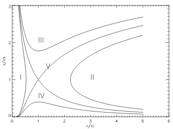
Figure 1.7: The solar wind velocity v as a function of radius r for various values of the constant C. The five different classes of solution are indicated by the labels I-V. cs is the sound speedvc and rc is the sonic radiusrc

and rewrite (1.25):

v2₋v_c21 v

dv dr = 2

v2 c

r2 (r−rc). (1.27)

Integrating (1.27) equation yields:

v vc 2 −ln v vc 2

= 4 ln

r rc

+ 4rc

r +C, (1.28)

Parker’s equation.

The various possible solutions to (1.28) depend on the constant C and are shown in Figure 1.7. While they are all mathematically valid most have unphysical properties. Solution I is double-valued which is unphysical as it implies the SW leaves the solar surface with sub-sonic velocities, reaches a maximum radius and returns to the surface at super-sonic velocities. Solution II is double-valued and never reaches the solar surface so is clearly unphysical. Solution III starts at super-sonic velocities at the solar surface which is not observed so this solution is neglected. Solution IV know as the ‘solar breeze’ because inspecting Figure 1.7 we see that as r _{→ ∞} that v _→ 0 thus at large distances we may

(38)

1. INTRODUCTION

approximate (1.28) with

−ln

v vc

2

≈4 ln

r rc

=_⇒ v

vc ≈

_r_c

r

2

=_⇒ r2v_≈r2_cvv = constant. (1.29)

Inserting this into the mass continuity equation ρ = const/r2v = const/r2_cvc the density

tends to a constant and as the plasma is isothermal the pressure must also be a finite constant. This is not physical as the extremely small ISM pressure cannot balance the SW pressure. Solution V crosses through a critical point at r = rc, v = vc called the

sonic point. This point can be used to constrain the integration constant C =₋3. Again inspecting Figure 1.7 we see as r_{→ ∞} thatvvc so (1.28) is approximated by

v vc

2

≈4 ln

r rc

=_⇒ v

vc ≈

2 s ln r rc . (1.30)

From the mass continuity equation the density is given by

ρ= const

r2_v ≈

const0

r2

r

ln_rr

c

(1.31)

so the density will tend to zero, and as the plasma is isothermal so will the pressure thus this solution can match the ISM pressure. So the Parker solar wind solution is given by solution V which starts off sub-sonically at the solar surface, the velocity increases monotonically with height, reaching the sound speed at the critical point (or sonic point), and propagates super-sonically thereafter. We can estimate the critical radius and velocity by assuming a typical temperature for the solar wind of T ≈ 106K, deriving vc ≈ 120 km s−1 and

rc= 12 R which corresponds to a solar wind velocity at 1 AU of 430 km s−1 very close to

the measured velocity of _∼400 km s−1. In 1959 the first indications of the presence of the solar wind came from the Russian Lunik III and Venus I spacecraft and was confirmed in 1962, just four years after its prediction, by Mariner II spacecraft measurements analysed by Neugebauer & Snyder (1962).

As the plasma-βof the solar wind is much larger than one, (see Figure 1.6) the magnetic field will be advected outward with the solar wind as the field lines are ‘frozen in’ (see Section 2.1.3). The combination of this radial advection with the rotation of the Sun forms what is known as the Parker spiral. If we assume that solar gravitation and solar wind acceleration can be neglected beyond some distance r0, then the radial outflow velocity

(vr) can be approximated by a constant v. In a spherical coordinate system which rotates

(39)

1.1 The Sun

with the Sun we can write the velocity components as:

vr=v, vθ= 0, vφ=ω(r−r0) sinθ (1.32)

whereωis the angular velocity of the Sun (ω= 2.7_×10−6_{rad s}−1_{). A differential equation}

for the velocity stream lines can be obtained fromv×dS= 0:

dr vr

= rdθ

vθ

= rsinθdφ

vφ

(1.33)

Integrating this equation fromr0 tor and from φ0 toφgives:

r r0 −

1₋ln

r r0

= v

r0ω

(φ₋φ0), (1.34)

when r > r0 this equation can be approximated by:

(r₋r0)≈

v

ω(φ−φ0) (1.35)

which is in the form of an Archimedean spiral shown in Figure 1.8.

As the magnetic field ‘frozen in’ to the flow and considering that ∇ ·B = 0 we may write:

Br(r, θ, φ) =B(θ, φ0)

_r

0

r

2

Bθ(r, θ, φ) = 0

Bφ(r, θ, φ) =B(θ, φ0)

_ω

v

(r−r0)

_r₀

r

2

sinθ

(1.36)

whereB(θ, φ0) is the magnetic field atr =r0. The angle of the magnetic field with respect

to the radial direction can be obtained from:

tanψ= Bφ

Br

=ω

v

(r−r0) sinθ (1.37)

and when r is large this is approximated by:

tanψ= Bφ

Br

=ωr

v

sinθ. (1.38)

Inserting typical values of the solar wind at Earth of v = 400 km s−1_, _ω _{= 2}_.₇_×₁₀−6

(40)

[image:40.612.129.445.123.431.2]

1. INTRODUCTION

Figure 1.8: The interplanetary magnetic field showing the Parker spiral geometry for a solar wind speed of 600 km s−1 _{and a field line starting at a Carrington longitude of 0}◦_.

rad s−1 _{and using}_r _{= 1 AU = 1}_.₅_×₁₀8_{km and sin(90}◦_{) = 1 we find} _ψ_∼₄₅◦ _{close to the}

measured value (M. Goossens, 2003).

It is now known that the solar wind consists of two components: the slow solar wind with typical 1 AU values for velocity, density, and temperature of_∼400 km s−1_,_∼_{10 cm}−3_,

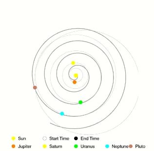
∼1.4_×105K respectively; and the fast solar wind with typical 1 AU values for velocity, density, and temperature of 800 km s−1,∼3 cm−3, and∼1.0×105K respectively originating from open magnetic field regions (see Figure 1.9). The two different speed streams can interact to form co-rotating interaction region (CIRs) where the fast wind ploughs into the slow solar wind and can form shocks. Another feature of the solar wind is the heliospheric current sheet (HCS) which separates the two opposite polarities of the Sun’s magnetic, field forming what is know as the ‘ballerina skirt’.

The solar wind cannot expand forever and eventually runs into the ISM at what is known as the termination shock, where the solar wind transitions back to sub-sonic

(41)

1.2 Coronal Mass Ejections

in SC 23, over Ulysses’ third orbit, compared to those taken during its first orbit at a very similar phase of cycle 22. We also examine the properties of the in-ecliptic solar wind, comparing long term trends in the low latitude Ulysses data with data from the Solar Wind Electron Proton Alpha Monitor (SWEPAM) [McComas et al., 1998b] on the Advanced Composition Explorer (ACE).

2. Observations

[7] Figures 1a – 1c show polar plots of the solar wind

speed over all three of Ulysses’ orbits. Underlying the SWOOPS data are composite images of the Sun and corona, which illustrate the solar conditions for each orbit: mini-mum in SC 22, maximini-mum in SC 23, and minimini-mum in SC 23, respectively. Figures 1a and 1b are essentially replots of figures by McComas et al. [1998a, 2003]. Figure 1d dis-plays the smoothed sunspot number (black) and averaged current sheet tilt relative to the solar equator (red), taken from the Wilcox Solar Observatory (WSO).

[8] Around minimum in SC 22, the band of solar wind

variability was narrow, and confined to low latitudes (_!30! to _!20! north) [Gosling et al., 1995, 1997;

McComas et al., 1998a]. This configuration was

consis-tent with the small dipole tilt angles seen at the time and confinement of the helmet streamers to low latitudes. In contrast, the tilt of the heliospheric current sheet has remained substantially higher thus far through the minimum of SC 23, even though the sunspot number declined to very low values. Figure 1c shows the comparable plot for Ulysses’ third orbit. Generally, Figures 1a and 1c look very similar except for the reversed solar magnetic field. Also note that the band of solar wind variability extends to somewhat higher latitudes in the third orbit observations. The brief low speed interval (_!5:30 position) in the otherwise fast PCH wind was caused by significant mass loading of the flow by comet McNaught [Neugebauer et al., 2007].

[9] Figure 2 shows a comparison of various plasma

properties taken as a function of heliolatitude for the PCH flows observed over Ulysses’ first and third orbits. From top to bottom, the plots show proton speed, proton density normalized by R2, proton temperature normalized by R [McComas et al., 2000], the alpha particle to proton ratio, and the full normalized momentum flux, or dynamic pressure, mp(npvp2 + 4nava2)(R/Ro)2. We separated the

one-hour averaged SWOOPS data into 4! bins in heliolatitude from 40! to 80!and calculated mean values (symbols) and ±1s variations (bars) for each bin.

[10] While there were small variations between the fast

and slow latitude scans (small vs. large symbols) and northern and southern PCH observations (circles vs. squares), the most significant differences in Figure 2 are clearly between first (red) and third (blue) orbits. The PCH solar wind observed in Ulysses’ third orbit is significantly slower, less dense and cooler than that observed in Ulysses’ first orbit. Of these, the speed shows the least difference, particularly at the highest latitudes, although in combination, these four-degree binned samples show a consistently lower speed in the third orbit. In addition, the speed also continued to show its characteristic, but still unexplained, increase of

!1 km s"1per degree of heliographic latitude [McComas et al., 2000, 2002, 2003]. Because the wind was slower and less dense, the dynamic pressure was also lower in the third orbit. In contrast to these bulk properties, however, the alpha to proton ratio, which is a measure of the plasma composi-tion, was essentially identical.

[11] Table 1 provides the mean values for selected plasma

parameters. All values were calculated by averaging all one-hour averaged data samples obtained above 40!heliolatitude. The columns show the first orbit mean value, the third orbit mean value, and the percentage change of the third orbit value compared to the first. The short interval around the comet McNaught encounter was removed so as not to bias the sample. Clearly, the PCH solar wind was

consis-Figure 1. (a – c) Polar plots of the solar wind speed, colored by IMF polarity for Ulysses’ three polar orbits colored to indicate measured magnetic polarity. In each, the earliest times are on the left (nine o’clock position) and progress around counterclockwise. (d) Contemporaneous values for the smoothed sunspot number (black) and heliospheric current sheet tilt (red), lined up to match Figures 1a – 1c. In Figures 1a – 1c, the solar wind speed is plotted over characteristic solar images for solar minimum for cycle 22 (8/17/96), solar maximum for cycle 23 (12/07/00), and solar minimum for cycle 23 (03/28/06). From the center out, we blend images from the Solar and Heliospheric Observatory (SOHO) Extreme ultraviolet Imaging Telescope (Fe XII at 1950 nm), the Mauna Loa K coronameter (700 – 950 nm), and the SOHO C2 white light coronagraph.

L18103 MCCOMAS ET AL.: WEAKER SOLAR WIND L18103

2 of 5

Figure 1.9: (a-c) Polar plots of solar wind speed with the magnetic field polarity indicated by colour for three Ulysses orbits. The background image are blended composites from SOHO/EIT 195 ˚A, the Mauna Load K coronameter and SOHO/LASCO C2. (d) Show smooth sunspot number and heliospheric current sheet tilt angle (McComaset al., 2008).

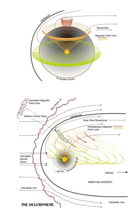
ities (Figure 1.10). The Voyager II spacecraft recently (and previously Voyager I) passed though this region at some 70 – 90 AU, details of these shock crossings can be found in Richardson et al. (2008), Burlaga et al. (2005) and Decker et al. (2008). Outside of the termination shock lies the heliosheath where the ISM and SW are in pressure balance, its outer boundary is the heliopause which also marks the edge of the Heliosphere. In this region the interaction between the ISM and SW causes turbulence and heating of plasma. As the Sun travels around our galaxy and encounters the ISM a bow shock is believed to from ahead of the heliopause (Figure 1.10).

1.2 Coronal Mass Ejections

“We define a coronal mass ejection to be an observable change in coronal structure that (1) occurs on a time scale between a few minutes and several

hours and (2) involves the appearance (and outward motion) of a new, discrete,

bright, white-light feature in the coronagraph field of view.”

-Hundhausen et al.(1984)

Coronal Mass Ejections (CMEs) are large scale eruptions of plasma and magnetic field which propagate from the Sun into the Heliosphere. A typical CME has a magnetic field strength of tens of nT, a mass in the range of 1013_–1016_{g (Vourlidas} _{et al.}_{, 2002) and}

(42)

1. INTRODUCTION

[image:42.612.153.373.196.537.2]

1. INTRODUCTION

Figure 1.11:The 3D structure of the heliospheric magnetic field. Figure courtesy of Steve Suess, NASA/MSFC.

28

Figure 1.10: Depiction of the Heliosphere and its prominent features. Shown are the spiralling magnetic field lines, termination shock, heliopause, and bow shock. Image courtesy of Steve Suess, NASA/MSFC.

(43)

1.2 Coronal Mass Ejections

Advanced Image Processing for STEREO

1

1. What is the question this proposal addresses?

Solar coronal mass ejections (CMEs) are spectacular eruptions of plasma and magnetic fields that drive space weather in the near-Earth environment. Despite nearly thirty years of study, the basic physics that expels these plasma clouds into the solar system is still not well understood. The Sun-Earth Connection Coronal & Heliospheric Investigation (SECCHI1_{) aboard NASA’s recently launched Solar Terrestrial Relations Observatory}

(STEREO2_{) is designed to explore various manifestations of the CME process in three}

dimensions. The SECCHI instrument compliment combines comparable solar disk, coronagraph, and heliospheric observations from two distinct views and is well suited to exploring the physics of CMEs, both at the source and during their propagation to Earth (Howard et al. 2002). This therefore offers us a unique opportunity to investigate the detailed physics involved in initiation and accelerating CMEs. We propose to develop advanced image processing methods to extract the evolving morphology and kinematics of CMEs and to compare these results with as yet unconfirmed predictions of theory.

1.1 Theoretical Models

From a theoretical perspective, several models have been proposed to describe the observed properties of CMEs shown in Figure 1. The two-dimensional flux-rope model was first proposed by Priest & Forbes (1990) and subsequently developed by Isenberg, Forbes & Demoulin (1993) and Forbes & Priest (1995). In this model, the CME is assumed to be initially located at the centre of a bi-polar field configuration as shown in Figure 2a. The field foot-point separation (!) is gradually decreased, and an eruption is triggered by a loss of equilibrium or instability in the field. The flux-rope then accelerates away from the surface as overlying fields are sequentially disconnected from the surface by magnetic reconnection (Figure 2b-d).

A more recent model that builds on the basic features of these two-dimensional ideas, is the three-dimensional magnetic flux-rope model of Krall et al.

(2001) and Chen & Krall (2003). They assumed that the kinematics of an erupting flux-rope could be described using the force-balance equation,

!

md

2_h

dt2="#P"$g+j%B, (1)

where h is the height, and the terms on the right describe gas pressure, gravity and the Lorentz force. Dropping the small gravitational force and initially small drag, the acceleration can be expressed as

! d2_h

dt2~

"p

2

[Rln(8R/af)]

2fR, (2)

where "pis the (poloidal) magnetic flux inside the tube,

fRthe force in the radial direction, af the flux-rope

radius, and R its radius of curvature (see Chen & Krall 2003 for details). The flux-rope acceleration is therefore dependent on its geometrical properties, including

1_{http://secchi.nrl.navy.mil} 2 http://stereo.gsfc.nasa.gov

Figure 1: The fundamental components of a CME observed by the LASCO coronagraph on the SOHO spacecraft. Front Cavity Core Occulting disk

Figure 1.11: The typical components of a CME observed by the LASCO coronagraph on SOHO spacecraft.

velocity between ∼10 – 2,000 km s−1 some times even reaching 3,500 km s−1 close to the Sun (Yashiroet al., 2004). At 1 AU, CME velocities (300 – 1,000 km s−1_{) tend to be closer}

to the solar wind speed (Gopalswamy, 2006; Lindsayet al., 1999; Wang et al., 2005). The energies associated with CMEs are of the order of 1024–1025J making CMEs the most energetic events on the Sun (Vourlidaset al., 2002). Although CMEs often exhibit a three-part structure which consists of a bright front followed by a dark cavity and bright core (see Figure 1.11), they may also exhibit more complex structures (Picket al., 2006). In fact less than_∼30% of CME events possess all the three parts (Webb & Hundhausen, 1987).

CMEs are know to be the most important driver of adverse space weather on Earth and in the near-Earth environment as well as on other planets (Prang´eet al., 2004; Schwenn

et al., 2005). The most famous phenomena associated with space weather is the Aurora

Borealis or Northern Lights (see Figure 1.12). The Aurora is caused by energetic particles traveling along the Earth’s magnetic field lines interacting with atoms (mainly nitrogen and oxygen) in the upper atmosphere producing emission (resonance or recombination).

(44)

1. INTRODUCTION

Figure 1.12: Two images of the aurora from Eielson Air Force Base at Bear Lake, Alaska (top) and from onboard the ISS (bottom). Images courtesy of Wikimedia Commons.

Propagation of coronal mass ejections in the inner heliosphere