Study on A Rolling Prediction Model of Power System Load Forecasting Based on Evolutionary SVM

(1)

Study on A Rolling Prediction Model of Power System

Load Forecasting Based on Evolutionary SVM

Zhang Lin

_{Ma Chao Liu Xianshan}

Abstract—A novel rolling prediction method is introduced, which was an evolutionary Support Vector Machines (SVM) algorithm based time series. The algorithm would resolve how short term power load could be forecasted accurately and rapidly. The power load system was an uncertain, nonlinear, dynamic and complicated system, so it was difficult to describe such a nonlinear characteristics of this system by traditional methods. The algorithm avoided traditional model of SVM to control the kernel function and parameters and found the local and global optimization with Simplex-Niche-Genetic algorithm, which was more generalized and its dependence on experience was weakened. At the same time, the numerical simulation proved the method rationality and was applied to predict the power system load base on the time characteristic. Therefore, considering time series could predict the power system load in sequence and enhance the efficiency and the capability of prediction to maintain power system reliability and stability so as to make prediction model agree with the load’s dynamic mechanical characteristic. And then, taking practical project as training samples to generalize and forecast the power system load, the result was satisfied, which illuminated forecasting accuracy was superior to traditional BP Neural Network. So prediction model put forward in the paper could get simulate result quickly and accurately, which provided a new thought for power system load forecasting and power system grid layout and construction.

Index Terms— Power Load forecasting；Simplex-Niche- Genetic algorithm；Support Vector Machines（SVM）；Time series

Ⅰ.INTRODUCTION

In the 1970s, Vapnik[1]presented statistical learning theory, and in the middle of 1990s, the theory developed rapidly and matured gradually so as to derive a novel universal machine learning method named Support Vector Machine(SVM). In recent years, SVM has been applied widely in modes identification including text identification, language identification and face identification and so on, and has also got favorable effect in the above fields.

Manuscript received July 5, 2007. This work was supported in part by the Chongqing Electric Power CORP.,

Zhang Lin is with the Chongqing Electric Power CORP., Chongqing 400014, China (phone:86-023-63680906; fax:86-023-63683120; e-mail: [email protected]).

Ma Chao is with the Chongqing Electric Power CORP., Chongqing 400014, China (phone: 86-023-63680821; fax:86-023-63680813; e-mail: [email protected]).

Liu Xianshan is with the College of Civil Engineering, Chongqing University,Chongqing,400044,China(phone:86-023-63680906;

fax:86-023-63683120; e-mail: [email protected]).

Taking many achievements in the field of practical prediction for instances, Zhu[2]designed SVM to predict chaotic time series with noise , and some authors[3-4] adopted SVM method to solve practical problems. And compared with intelligent methods such as artificial neural network and genetic algorithm, SVM is superiority to above methods because it isn’t easily got into local optimization and the ability of generalization is also improved largely. However, the ability of generalization depends on kernel function and special parameters to some degree, so it’s important to decide the factors rationally. And Simplex-Niche-Genetic algorithm is an evolutionary method considering no gradient based on hunting multipoint information and has the merits of rapid local convergence, global optimization and parallelism and so on. So combined with the optimum method called Simplex-Niche-Genetic algorithm and SVM, an evolutionary SVM method is brought forward in the paper, which may realize nonlinear and global optimization ability.

In order to prove the feasibility of evolutionary SVM method, numerical simulation is done for a nonlinear function, and at the meantime, applying the method to predict the power system load. In virtue of load series being formed under all kinds of comprehensive factors including a great deal of evolutionary information of the power system load to make balance of the power supply and demand prediction very complicated, correction of the example’s results should prove that evolutionary SVM method owns strong nonlinear and global optimization ability.

Ⅱ_{. THEORY OF SUPPORT VECTOR MACHINE}

The basic idea is changing the input space to a high dimensional space through nonlinear transformation based on inner product function to look for precise description for the nonlinear relationship between input variables and output variables in the high dimensional space. SVM is a method adopting minimum principle of structural risk which is superiority to traditional intelligent methods. And the algorithm is a convex quadratic optimization, so the ultimate solution is the global optimization and can solve many practical problems owning small samples, nonlinear and high dimensions.

For training samples{ , }x yi i li=1,xi∈Rnrepresents

input variables, yi∈Rrepresents corresponding output

(2)

space to output space to make f x( )=y. So the aim of SVM is finding regression function given by the following formula:

( ) ( )

y= f x = ω⋅ +x b (1) In the formula, ω∈_Rnis weight factors, _x∈_Rn

represents input variables; b∈Ris threshold value. According to statistical theory, SVM decides regression function through minimizing goal function which is expressed by the following formulas:

2

1

1 1

M in{ ( ( ))}

2

l

i i

i

C v l

ω ε ξ ξ∗

=

+ ⋅ +

∑

+ (2)

s.t. ((ω⋅xi)+ − ≤ +b) yi ε ξi (3)

(( ) )

i i

y − ω⋅x +b ≤ +ε ξ_i∗ (4) 0

i

ξ∗_≥ _， _ε_≥₀₍₅₎ In the formula(2)~(5), C , ν represent weight parameters to balance the complex item expressed by

2 1

2 ω and training error terms of above-mentioned model, ε is insensitive loss function, ξ ，ξ_i∗_represent relaxation factors.

And then, corresponding multipliers such as ( )

i

α∗ _，

i

α ，η_i，η_i( )∗ ，β_≥0_{are lead to the above-mentioned}

model according to Lagrange algorithm for restrained conditions to get the following formula:

2 ( ) ( ) ( ) 1 ( ,b, , , , , , , , )

2

Lω α α β ξ ξ ε η η∗ ∗ ∗ = ω +Cνε+

1 1 1

( ) ( ) (

l l l

i i i i i i i i i

i i i

C

y

l ξ ξ βε η ξ η ξ α ξ

∗ ∗ ∗

= = =

+ − − + − + −

∑

1

( i) ) l i( i ( i) i )

i

x b x b y

ω ε α ξ∗ ∗ ω ε

=

⋅ − + −

∑

+ ⋅ + − + (6)

In order to minimize the formula (2), the saddle points should be solved through minimizing variables such as ω，ε，b，ξ ，ξ_i∗ and maximizing variables such as ( )

i

α∗ _，

i

α ，β，η_i，η_i( )∗ . And then, four equations are

obtained as follows according above theory.

1

( )

l

i i i

i

x

ω α α∗

=

∑

− ⋅ (7)

1

( ) 0

l

i i

i

C ν α α∗ β =

⋅ −

∑

+ − = (8)

1

( ) 0

l

i i

i

α α∗

=

− =

∑

(9)

( ) ( ) ₀

i i

C

l α η ∗ ∗

− − = (10) Finally, regression function of SVM is got as following formula through solving above-mentioned equations.

l *

1

( ) ( i i)( , )i i

f x a a x x b =

=

∑

− + (11)

For nonlinear problems, solving original models may be changed to be solving linear problems of high dimensional space through nonlinear transformation. Moreover, inner product calculation for linear problems

in the high dimensional space may be in place of as follows.

( , )i j ( ) ( )i j

K x x =φ x φ x (12) Kernel function may be realized through the functions of original space so that it isn’t necessary to require specific formation of nonlinear transformation. Therefore, regression equation of above nonlinear problem is expressed by the following formula:

*

1

( ) l ( i i) ( , )i i

f x a a K x x b =

=

∑

− + (13)

According to the characteristic of SVM regression function, only minority of (α αi∗− i)are not equal to zero, and corresponding vectors of these parameters are called support vectors which decide the regression function

( )

f x completely.

As far as kernel functions are concerned, more than ten kinds of kernel functions have been constructed in recent years, common kernel functions are following formulas:

1）_{Polynomial kernel function}

( , ) ( 1)d

K x y = ⋅ +x y ， d=1,2, ,_L (14) 2）_{Radial basis kernel function}

2

2 ( , ) exp( x y ) K x y

σ −

= − (15) 3）_{Sigmoid kernel function}

( , ) tanh[ ( ) ]

K x y = b⋅ ⋅ +x y θ (16)

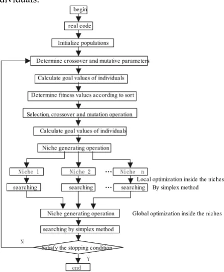
Ⅲ. SIMPLEX-NICHE-GENETIC ALGORITHM Niche is a kind of organizing function under specific conditions in biology, and simplex method is an optimization method with no gradient which has strong local optimization ability and can rapidly converge to local optimization values near initial values. Therefore, combined with above-mentioned methods, their superiority will be showed to solve nonlinear multi-peaked optimization problems rapidly and correctly which can overcome prematurity of traditional genetic algorithm and slow convergence of niche-genetic algorithm. Process chart of Simplex-niche-genetic algorithm adopted in the paper is showed as figure 1 and basic steps are expressed as follows:

a) Initialize populations. Set counter n equal to 1,and generate initial populations P(n) with real codes which number is M.

b) Set parameters. Determine coherent parameters such as crossing probability, mutative probability and niche radius and etc. And then, add counter n to 1 and compare the current value of n with maximum circulation. If counter n reaches maximum circulation, turn to step 9).

c) Calculate fitness values of individual. Calculate goal function value of individual at first, and then, ascending sort is done according to goal function value and determine fitness values of individual by sequence. At the same time, save N individuals(N<M).

d) Genetic operation. Selection ,crossover and mutation operation are done for populations P(t) to generate new populations P(n)’_.

(3)

(M+N) individuals. And then, calculate goal values of new populations and Euler distance between individuals is calculated by following formula:

(

)

∑

= − =

− n

k

jk ik j

i x x

n X X

1

2

1

⎟⎟ ⎠ ⎞ ⎜⎜

⎝ ⎛

+ +

=

− + =

N M i

j

N M i

, , 1

1 ,

, 2 , 1

L L

(17) If value of formula (17) is less than niche radius, compare goal values of Xi and Xj. And then, punish the individual with bigger value to make it be equal to G.

f) Local optimization inside the niche by simplex method. Firstly, calculate individual numbers of every niche population. And then, search S times through simplex method when some niche population includes more than two individuals. Finally, generate a new population as current population.

g) Niche operation. Niche operation is made for new populations, and then reserve N local optimization having been found according to ascending sort of goal function values.

8) Global optimization inside the niche by simplex method. Search for S times for N local optimization individuals of niche, and then, substitute poorer individuals for the better to form a new population. Finally, merge the above new population and N individuals deserved previously to form another new population, then turn to 2).

9) Convergence. Put out all the optimizing individuals.

real code

Initialize populations

Determine crossover and mutative parameters、

Determine fitness values according to sort

Selection, crossover and mutation operation

Niche generating operation

Niche 1 Niche 2 Niche n

searching searching

…

Satisfy the stopping condition

end Y N

begin

Local optimization inside the niches Calculate goal values of individuals

searching By simplex method

Global optimization inside the niches Niche generating operation

[image:3.595.303.549.185.259.2]

searching by simplex method Calculate goal values of individuals

Fig. 1 Process chart of Simplex-niche-genetic algorithm

Ⅳ. SIMULATION CALCULATION

Code has been written according to the theory mentioned above. In order to prove its superiority to artificial neural network, a Sine function is simulated by evolutionary SVM and artificial neural network.

Divide the period of Sine function into 20 divisions as sample modes. Set input samples as X_i =i/20.0and output samples as

5 . 0 ) * * 2 sin( * 4 . 0 =

Yi π Xi + ，(i=1,...,20). (18)

And then, calculate the values of training sample on the same initial conditions with two methods mentioned above separately. Finally, set two input samples which are a1=0.225 and a2=0.675 as simulating samples ,the results is showed as table 1.

[image:3.595.65.285.360.627.2]

According to the results showed in table 1, iteration time of algorithm brought forward in the paper is less and simulation values are more accurate than BP network. Especially, when energy function values is less and less, BP network isn’t easy to converge, however , evolutionary SVM may skip local optimization and easily reach global optimization and convergence.

Table 1 comparison with evolutionary SVM and BP

（Back Propagation）network

methods evolutionary SVM BP network convergence 1.5e-3 1.0e-6 1.5e-3 _1.0e-6 Training time (s) <1 10 2805

a1 0.89504 0.89505 0.89491 Simulation

values a2 0.14354 0.14357 0.14352

Can’t converge

Ⅴ. ROLLING PREDICTION MODEL OF THE POWER SYSTEM LOAD

BE CONSTRUCTED AND APPLIED

A. Data model building based on time series

According to the characteristic of power load in some province, the typical data of month power load could be selected to construct the model. The data of month power load have two observable locomotive characteristic: trend and periodicity, the periodicity is 12 months. Define: yt as the observed value of the average load during t month, Gt as the trend component of the average load during t month,

Η

t as the circle component

of the average load during t month,

E

tas random noise

(

_σ

=0), which include the measure noise and model error.

We can describe the load model which has trend and seasonal periodicity characteristics by (19)

t t t t

y =G H E ₍₁₉₎ Define the sequences of the average month load are

y

1

,

y

2

y

3

...

y

T, T is the length of the sequence of the

data. If the year of observed value sequence is N, there is a linear relation as:

T

=

12 N

. Use the moving average method of mid value, the trend component can be abstract from the complex relationship as:

11 11 1

0 0

1 [ ]

24

t t i t i

i i

G y₊ y_{++ +} = =

=

∑

+

∑

(20)

1,2, , 12 t= _LT−

The equation (20) avoids the seasonal fluctuation, which means the periodicity is 12 month and digital filter based on the double moving-average model whose symmetric center is

t

.

After digital filtering by the model, we get rid of the circle component. So the trend component is decomposed from the sequences and be constructed by

y

tand

G

tin the

(4)

seasonal circle component taking into consideration of the measure noise and model error. rand noise could be described as the following equipment:

H Et t=y Gt/ t (21)

B. Theory of rolling prediction

Error will increase rapidly with the prediction steps increasing according to prediction theory. Therefore, rolling prediction method will be adopted in order to take good use of measuring information to improve prediction veracity. The basic theory of the method is expressed as follows. Firstly, set predicting time series as {xi} and the

best history points as p as well as prediction steps as m.( p，_{m is determined by trial calculation).There are n}

monitoring values currently. Rolling prediction data of the first step is {xn- p+1，x2n-p+2，…，xn} and {xn+1，xn+2，…，

xn+m} is the data after n step. With the back data which

the number is m getting, delete {x1，x2，…， xm} of the

front data and form a new series as {xm+1，xm+2，…，xn+m}

to predict values of the next step. So rolling prediction uses up-to-date monitoring data every time so as to overcome excessive prediction steps and make real-time trace possible.

C. Rolling prediction model of the power system load Because the load system is an uncertainty non-linear system accompanied with many factors, to unveiled the problem, we assume n

i

R

x

∈

as the main factor which

affected the power load forecasting, and the simplification is proved be reasonable. Then

y

t is load

forecasting data sequences. Prediction model problem can be simplified as:

:

f

R

n

→

R

)

(

i i

f

x

y

=

(i=1,2,…k) (22)

Rn_{is trend component and the circle component,} while R is the forecasting value. Firstly, get load series {xi} with time according to monitoring values, and then,

predict the time series which is {xi，xi+1，…，xi+p-1} at time

p and load series at time i+p expressed as xi+1=f{xi，

xi+1，…，xi+p-1}. In the formula, f() is a nonlinear function

which illustrates nonlinear relationship of time series. According to SVM theory, nonlinear relationship above mentioned may be got by training n actual data. Therefore, prediction model of the power system load load is expressed as following formula:

(

)

K

(

X

)

b

X

f

n m i

p n

i

i i m

n

=

−

+

−

=

∗

+

)

∑

,

(

1

α

(23)

In the formula:

f

(

X

n+m

)

is load value at time

n+m,

X

n+m is load value before time n+m,

Xi

is

load value before time p+i,

K

(

x

n+m

,

x

i

)

is kernel

function.

Finally, optimizing SVM is got through optimization method in the paper, and then, evolutionary SVM of the power system load prediction will be determined based on time series.

D. Parameter of model and validating the forecasting value

We selected 120 samples from the load sequence in 1991~2000 years. Firstly, we use the data of load of

August, 1991~2000 as train sample. Parameter C and kernel function should be selected to construct the model based on the aforementioned theory.

Secondly, we select the

σ

=53,C=110 by SVM iterative calculation.

And then, calculate the values of training sample on the same initial conditions with two methods mentioned above separately. Finally, set two input samples as simulating samples, the results is showed as table 2.

[image:4.595.304.550.248.437.2]

According to the results showed in table 2, iteration time of algorithm brought forward in the paper is less and simulation values are more accurate than BP network. Especially, when energy function values is less and less, BP network isn’t easy to converge.However, evolutionary SVM may skip local optimization and easily reach global optimization and convergence.

Table 2 comparison with evolutionary SVM and BP network of power load

DATE(Year.Month) 2000.9 2000.10 2000.11 2000.12 Actual power load /MW 6082.490 6077.750 5799.820 6181.060 Data of load forecasting by the

traditional time series method

(MW) 5847.750 5870.235 5208.318 6792.961 The relative error of the

traditional time series method(%)

3.859 3.414 10.2339 9.899 The data of load forecasting by

the classical BP network (MW) 6052.981 5994.530 5710.741 6408.812 The relative error of the

classical BP network (%) 0.4851 1.369 1.5359 3.6847 The data of load forecasting by

Evolutionary SVM based time

series(MW) 6075.101 6071.424 5769.215 6275.153 The relative error of load

forecasting by Evolutionary SVM based time series (%)

0.1215 0.1041 0.5277 1.5223

Ⅵ. CONLUSIONS

1)Evolutionary SVM based on simples-niche-genetic algorithm may avoid parameters selection artificially and blindly to improve the precision and generalization ability of the model.

2) Evolutionary SVM owns fault-tolerant ability and fast convergence velocity, and can get global optimization to approach the accrual values.

3) Rolling prediction can real-time monitor construction to service for the stability of structures according to the project, which provides effective method for project design and construction

4) Precision is limited by all kinds of factors, so multi-factor will be considered for load forecasting model.

Ⅶ. REFERENCES

[1] Vapnik V N．_{Essence of statistical studying theory}

[M]．_{Beijing publisher}，₂₀₀₀．

[2] ZHU J Y，_eta1．_{Time series prediction via new support}

vector machine[J]．_{Proceedings of the First International}

Conference on Machine Learning arid Cybernetics．₂₀₀₂：

(5)

[3] Rosen, Scott L.，_Harmonosky，_{Catherine M.}。_An

improved simulated annealing simulation optimization method for discrete parameter stochastic systems[J], Computers and Operations Research，_{2005,32(2) , 343-358}。

[4] _{Martí, Rafael;}，_El-Fallahi，_Abdellah。_{Multilayer neural}

networks：_{an experimental evaluation of on-line training}

methods[J]，_{Computers and Operations Research ,2004,31(9) ,}

1491-1513.

[5] Chow T W S，_{Leung C T}．_{Neural network based}

short-term load forecasting using weather compensation[J]．_{IEEE Trans on Power Systems}，₁₉₉₆，₁₁₍₄₎：

1736-1742

[6] Alfuhaid A S，_{El2SayedM A}，_{Mahmoud M S}．_Cascaded

artificial neural networks for short-term load forecasting[J]．_{IEEE Trans on Power Systems}，₁₉₉₇，₁₂₍₄₎：

1524-1529．

[7] Mohan Saini，_L．_{Kumar Soni}，_M．_{Artificial neural}

network-based peak load forecasting using conjugate gradient methods[J]．_{IEEE Trans on Power Systems}，₂₀₀₂，₁₇₍₃₎：

907-912．

[8] Mukherjee S, Nonlinear prediction of chaotic time series using support vector machines[J]. Neural Networks for Signal Processing Ⅶ，₁₉₉₇：_511-520．

Author Introduction:

Zhang Lin, He received the PHD degree from the Institute of Electronics, Chinese Academy of Sciences in 2006. His main research fields are power system stability and control.

Email: [email protected] [email protected]