Abstract—In this study, a self-tuning output recurrent cerebellar model articulation controller (SORCMAC) is investigated to control a two-wheeled robot. Since it captures the system dynamics, the proposed SORCMAC has superior capability to the conventional cerebellar model articulation controller in efficient learning mechanism and dynamic response. The dynamic gradient descent method is also adopted to online adjust the SORCMAC parameters. Finally, the effectiveness of the proposed control system is verified by the simulations of two-wheeled robot control. Simulation results show that the two-wheeled robot can be controlled stably with uncertainty disturbance by using the proposed SORCMAC.
Index Terms— SORCMAC, two-wheeled robot, gradient descent method.
I. INTRODUCTION
In the past several years, there are several literatures to study the topic “wheeled robot”. The main topic of this research is how to keep the robot’s balance. Such a system would become a primary tool for studying balance in active balancing system. It is also to be an important precursor to the field of legged machines and locomotion studies for robotics. There are many researches in this filed. In [1], a trajectory tracking algorithm based on a linear state space model was proposed to control mobile robot. Graser et al. [2] used Newtonian approach and linearization method to get a dynamic model to design a controller for a mobile. In [3], a dynamic model was derived with respect to the wheel motor torques as input while taking the nonholonomic no-slip constrains into considerations. Furthermore, two controllers were proposed to stabilize the vehicle’s pitch and position.
Until now, at least one commercial product is available such as“Segway”.
Modern control system often requires high-speed high-accuracy linear motions. These linear motions are usually realized using the rotary motors with a mechanical transmission, such as reduction gears and lead screw. These
Manuscript received December 30, 2008. This work was supported by the National Science Council of Taiwan, R.O.C. under the Grant NSC96-2221-E-155-072
C.H. Chiu is with Department of Electrical Engineering, Yuan-Ze
University, Chung-li, Taoyuan 320, Taiwan. (e-mail:
W.R. Tsai is with Department of Electrical Engineering, Chung Yuan Christian University, Chung-li, Taoyuan 320, Taiwan.
M.H. Chou is with Department of Electrical Engineering, Yuan-Ze University, Chung-li, Taoyuan 320, Taiwan.
Y. F. Peng is with the Electrical Engineering Department, University of
Ching-Yun, Chung-Li, Tao-Yuan, 320, Taiwan, R.O.C. (e-mail:
transmission mechanisms not only significantly reduce the linear motion speed and dynamic response, but also introduce the backlash and large friction. A two-wheeled robot can besimply considered as an inverted pendulum on a two coaxial wheels which have independent drives. This system is composed of a chassis carrying a dc motor coupled to a gearbox for each wheel. The two dc motors are all the rotary motors. It is obviously the transmission loss exists. Therefore, its mathematical model will be complex and the motor parameters are time-varying due to increasing in temperature and changing in motor drive operating condition [4,5]. For control viewpoint, the conventional control technologies always need a good understanding of the plant models. Since a two-wheeled robot dynamic model is difficult to obtain, it is very difficult to control a two-wheeled robot using the conventional control technologies. In recent years, many advanced control techniques have been adopted for a two-wheeled robot control [1-3,6]; however, most of these methods need the plant model and some of these design procedures are overly complex.
Recently, many researches have been done on the applications of neural networks (NNs) for identification and control of dynamic systems [7-12]. Many authors have suggested NNs as powerful building blocks for a wide class of complex nonlinear system control strategies when there exists no complete model information or, even, a controlled plant is considered as a “black box” [7]. According to the structure, the NNs can be mainly classified as feedforward neural networks (FNNs) [8], [9] and recurrent neural networks (RNNs) [10,11]. The most useful property of NNs is their ability to uniformly approximate arbitrary input-output linear or nonlinear mappings on closed subsets. Based on this property, the NN-based controllers have been developed to compensate the effects of nonlinearities and system uncertainties in control system, so that the stability, convergence and robustness of the system can be improved. Moreover, RNN has capabilities superior to FNN, such as the dynamic response and information storing ability [10,11]. Since an RNN has an internal feedback loop, it captures the dynamic response of system with external feedback through delays. Thus, the RNN is a dynamic mapping and demonstrates good control performance in presence of unmodelled dynamics. However, no matter FNNs or RNNs, the learning is slow since all the weights are updated during each learning cycle. Therefore, the effectiveness of NN is limited in problems requiring on-line learning.
The cerebellar model articulation controller (CMAC) has been adopted widely for the closed-loop control of complex dynamical systems owing to its fast learning property, good
Two-wheeled Robot Control Based on
Self-tuning Output Recurrent CMAC
generalization capability, and simple computation [13,14]. The CMAC is a non-fully connected perceptron-like
associative memory network with overlapping
receptive-fields. The application of CMAC is not only limited to control problem but also to model-free function approximation. This network has been already validated that it can approximate a nonlinear function over a domain of interest to any desired accuracy. The advantages of using CMAC over conventional NN in many practical applications have been presented in recent literatures [15-16]. The conventional CMAC uses constant binary or triangular receptive-field basis functions. The disadvantage is that their derivative information is not preserved. For acquiring the derivative information of input and output variables, Chiang and Lin developed a CMAC with differentiable Gaussian receptive-field basis function, and provided the convergence analyses of this network [17]. In [18], an optimal CMAC has been proposed for the robot manipulator control. However, the major drawback of existing CMAC is that they belong to static networks. In other words, the application domain of CMAC will be limited to static mapping due to its feedforward network structure [19,20].
In this study, an self-tuning output recurrent cerebellar model articulation controller for a two-wheeled robot is investigated. Its architecture is a modified model of the conventional CMAC network to attain a small number of receptive-fields for capturing the system dynamics and converting the static CMAC into a dynamic one. Since it captures the dynamic response, the SORCMAC will demonstrate good control performance in presence of unmodelled system. The parameters of SORCMAC are on-line tuned by the derived adaptive laws automatically. Finally, simulation results show the proposed SORCMAC can move the robot forward and back ward stably with the uncertainty disturbance.
II. ARCHITECTURE OF TWO-WHEELED ROBOT
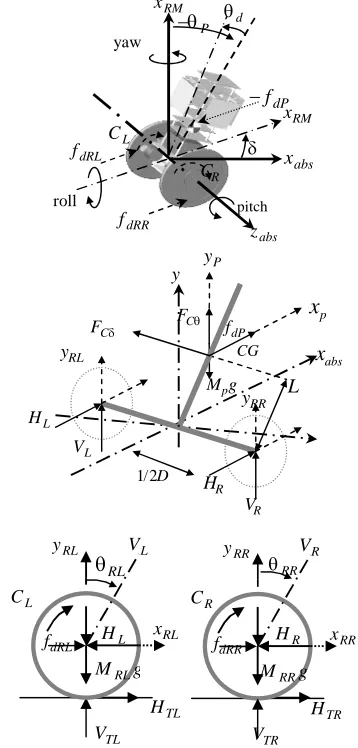
Figure 1 shows the robot with its three degree of freedom. The robot can be able to rotate around the z axis and its vertical axis. The whole system needs six state space variables to fully describe the dynamics of three degree of freedom [2]. The movement of the rotation around the z axis (pitch) can be described by the angle P and the corresponding angular velocityP. The linear movement of the chassis is the position xRM and the speed vRM .
Moreover, the robot can rotate around its vertical axis (yaw) with the associated angle and angular velocity .
dP
f ,fdRL and fdRR are the forces applied to the center of
gravity of the robot, to the center of the left wheel, to the center of the left wheel, respectively [2]. The dynamic mathematical model of the left-hand wheel can be described as follow: [2]
TL L dRL RL
RLM f H H
x
(1)
L RLg TL RL
RLM V M V
y
(2)
R H C
JRL L TL
RL
(3)
where JRLis the moment of inertia of the rotating masses
with respect to the z axis; MRLis the mass of the rotating
masses connected to the left and right wheels;JPis moment
of inertia of the chassis with respect to the z axis;Jpis
moment of inertia of the chassis with respect to the z axis;M is mass of the chassis;p
R : Radius of the wheels; D is lateral distance between the contact patches of the wheels;L is distance between the z axis and CG of the chassis. For the chassis,
L R dP p
pM f H H
x
(4)
C Pg L R p
pM V V M F
y
(5)
) (
cos ) (
sin ) (
R L
P R
L P L
R P P
C C
L H H L
V V J
(6)
2 )
(H H D
JP L R
(7)
where HL,HR,HTL,HTR,VL,VR,VTL, and VTR represent
[image:2.612.334.513.294.668.2]reaction forces between the different free bodies.
Fig. 1 Two-wheeled robot with its three degree of freedom
Obviously, the linear motion is realized using the rotary motors with reduction gears. These reduction gears not only significantly reduce the linear motion speed and dynamic response, but also introduce the backlash and large friction. It
TR V RR
y VR
RR
R C
TR H
RR x
g MRR
R H dRR f
TL H
RL x
TL V L
C
RL RL
y VL
g MRL
L H dRL f
roll pitch
yaw RM x
abs x P
d
RM x
dRR f
dP f
L C dRL
f
R C
abs z
L
H
L
V
D 2 / 1
R H
R
V L
RR y
g Mp
RL
x
RLy
abs
x
CGp
x
dPf
C
F
P y y
C
is obviously the transmission loss exists. Therefore, the mathematical model of such a system is complex and the motor parameters are time-varying due to increasing in temperature and changing in motor drive operating condition. For control viewpoint, the conventional control technologies always need a good understanding of the plant models. Since the accurate dynamic model is difficult to obtain, it is very difficult to control a two-wheeled robot using the conventional control technologies.
In this study, a model free self-tuning output recurrent cerebellar model articulation controller for a two-wheeled robot is investigated.
III. SORCMAC CONTROL SYSTEM
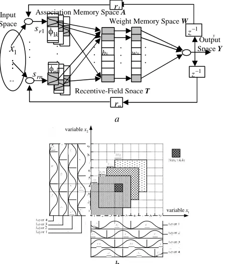
An SORCMAC control system is proposed in this section. The configuration of the proposed control system is shown in Fig. 2, where the reference angle signal is specified by a reference model following a command input
*
and p is the angle output of the two-wheeled robot
system. Moreover, the reference signal is specified by a reference model following a position command input x andm
the position output of the robot x. Clearly, is obtained from the robot’s position error. It is a virtual angle which is used to move the robot forward or backward to the target position. In this paper, a virtual angle can be gotten as
)) ( ) ( ( )
(N kx xm N x N
where k is a small positivex
constant. Obviously, ( N) will be zero when x(N) equals toxm(N). It means that the robot moves to the target position already. The inputs of SORCMAC are the mix angle tracking error of the robot’s bodyem(N)(N)p(N)(N) and
[image:3.612.314.539.402.665.2]change-of-error em(N)em(N)em(N1); the output of SORCMAC is the control signal
u
. Here, the model of the robot system is unknown.Fig. 2 Block diagram of two-wheeled robot control system
3.1 Description of ORCMAC
An output recurrent cerebellar model articulation controller (ORCMAC) is proposed and shown in Fig. 3a. The signal propagation and the basic function in each space are introduced as follows.
1) Input space X: For a givenx[x1,x2,,xn]T n, each input state variable x must be quantized into discretei
regions (called elements) according to given control space. The number of elements, n , is termed as a resolution.E 2) Association memory space A: Several elements can be accumulated as a block, the number of blocks, nB, in
ORCMAC is usually greater than two. The A denotes an association memory space with nA ( nAnnB ) components. In this space, each block performs a receptive-field basis function, which can be defined as rectangular or triangular or any continuously bounded function (e.g., Gaussian [18], [19] or B-spline [13], [21]). The Gaussian function is adopted here as the receptive-field basis function, which can be represented as
exp ( 2 )2
ik ik rik ik
v m x
, for k1,2,nB (8)
whereik represents the kth block of the ith input x with thei mean m and varianceik v . In addition, the input of thisik block for discrete time N can be represented as
) 1 ( ) ( )
(N x N r y N
xri i i (9)
where r is the recurrent weight of the recurrent unit. It isi
clear that the input of this block contains the memory terms )
1 (N
y , which store the past information of the network. This is the apparent difference between the proposed ORCMAC and the conventional CMAC. Figure 3b depicts the schematic diagram of two-dimensional ORCMAC operations with nE 9 and 4 ( is the number of elements in a complete block).
a
1
variable x
2
variable x
b
Fig. 3 a Architecture of SORCMAC, b A two-dimensional SORCMAC with 4 and nE 9
3) Receptive-field space T: The number of receptive-field,
R
n , is equal to nB in this study. Each location of A
Output Space Y
y
n
x
x
1
k
1
nk
bk wk
...
Input Space
X
Association Memory Space A
Receptive-Field Space T
Weight Memory Space W
... ... ...
1
z
1
z r1
... sr1
rn s
rn
*
+
u
p
r v
m w
P P
P P
, , , m
m e e ,
m m e e ,
m m e
e , k ik ik ik
r v m
w
, , ,
r v m w , , ,
p
m e
Two-wheeled robot system
On-line learning algorithm
Propagation error term
Optimal learning-rate
Referenc e model
RCMAC Reference
model
m x x
[image:3.612.79.283.463.609.2]corresponds to a receptive-field. The multidimensional receptive-field function is defined as
n i ik ik rik n i ik k k k k v m x b 1 2 2 1 ) ( exp ) , , ,(xm v r (10)
where bk is associated with the kth receptive-field,
n T nk k k
k [m1 ,m2 ,,m ]
m , [ 1 , 2 , ] ,
T nk k k
k v v v
v
n
and rk [r1,r2,,rn]T n. The multidimensional receptive-field function can be expressed in a vector form as
T n k bR
b
b , , , , ]
[ ) , , ,
( 1
x m v r (11)
where R R nn T T n T k
T
[m1, ,m , ,m ]
m , v[v1T,,
R R nn T T n T
k, ,v ]
v and R
R nn T T n T k
T
[r1 , ,r , ,r ]
r .
4) Weight memory space W: Each location of T to a particular adjustable value in the weight memory space can be expressed
as R R n T n k w w
w
[ 1,, ,, ]
w where w denotes thek
connecting weight value of the output associated with the kth receptive-field.
5) Output space Y: The output of ORCMAC is the algebraic sum of the activated weights in the weight memory space, and is expressed as
R n k k k k k kT w b
y 1 ) , , , ( ) , , ,
(xmv r x m v r
w (12)
A two-dimensional ORCMAC is shown in Fig. 8b.
3.2 On-line learning algorithm
Selections of the connective weight w , recurrent weight
r , mean m and variance v of the receptive-field basis
functions will significantly affect the performance of ORCMAC. Inappropriate recurrent weights and receptive-field basis functions will degrade the ORCMAC learning performance. For achieving effective learning, an on-line learning algorithm, which is derived using the supervised gradient descent method, is introduced so that it can real-time adjust the recurrent weights and means and variances of the receptive-field basis functions. Define the cost function E as
2 2 2 1 ) ( 2 1 m p e
E (13)
The error term to be propagated is given by
u e u e e E u E p m p p m m p (14)
and the learning algorithm, based on gradient descent method for w , can be derived ask
k p w k w k w k b w u u E w E
w
(15)
where the positive factor w is the learning-rate for the
output weight w . The connective weight can be updatedk
according to the following equation: ) ( ) ( ) 1
(N w N w N
wk k k (16)
Moreover, the mean, variance and recurrent weight of the Gaussian receptive-field basis functions can be also adjusted in the following equation:
2 ) ( 2 ik ik ri k k p m ik m ik v m x b w m E
m
(17)
3 2 ) ( 2 ik ik ri k k p v ik v ik v m x b w v E
v
(18)
) 1 ( 1
y N
r r E r i p r i r
i (19)
where the positive factors m, v and r are the
learning-rates for the mean, variance and recurrent weight, respectively. Then the updated laws of mean, variance and recurrent weight are given as follows:
) ( ) ( ) 1
(N m N m N
mik ik ik (20)
) ( ) ( ) 1
(N v N v N
vik ik ik (21)
) ( ) ( ) 1
(N r N r N
ri i i (22)
If the plant model is obtainable, then the Jacobian of the system p u can be calculated. If the plant model is unknown, then p u cannot be obtained. Although intelligent identifier [10] can be implemented to identify the system model, heavy computation effort is required. A simple approximation of the propagation error term of the system can be used as follows [22]:
m m p e e
(23)
According to Theorem 1, the optimal learning-rate parameters can be gotten automatically and the convergence of tracking error is guaranteed.
IV. SIMULATIONS
[image:4.612.325.536.52.139.2]In this section, the simulations of the two-wheeled robot using the effective SORCMAC based on the proposed learning laws will be demonstrated. The description of the two-wheeled robot and its model are shown in Section 2. For all the simulations shown in this section, the parameter values of the robot are listed in Table 1 [3].
Table 1. Simulation parameters
b
M 35 Kg Ixx 2.1073 kg
m
2w
M 5 Kg Iyy 1.8299 kg
m
2R 0.25 m Izz 0.6490 kg
m
2z
c
R, 3R m Iwa 0.1563 kgm
2b 0.2 m Iwd 0.0781 kg
m
2The SORCMAC used in this study can be characterized as 4
, nE 5 , nB nR 24 . The inputs of the SORCMAC are the angle error of the robot’s body, e , andm
the change rate of the angle error, em. The receptive-field
basis functions are chosen asik(xri)exp[(xrik mik)2
]
/vik2 for i1,2andk1,2,,8. Additionally, The initial values of the parameters are chosen asr10.1,r2 0.1,
4
1
i
m , mi23 , mi31 , mi40.5 , mi50.5 ,
1
6
i
m ,mi73,mi8 4and vik 2 for all i and k .
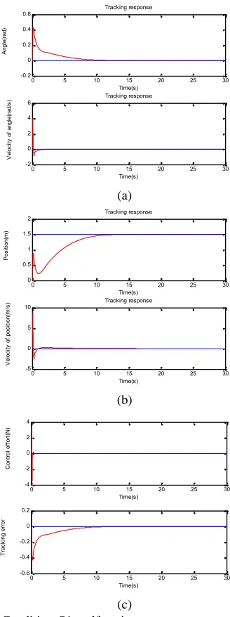
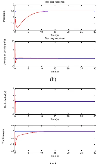
SORCMAC, several simulation conditions are adopted. Moreover, the external disturbance d is added and is assumed to be 0.0873 during the all simulations. Fig. 4 is the performance of the robot in the normal condition. The target position of the robot is 1.5m. Also, Conditions S1 denotes the extra mass 5Kg is added on the robot. Conditions S2 denotes the existence of the extra mass as S1 with the difference center of mass of the robot body about 3L (half length of the robot). The simulation results are given in Fig. 5 to Fig. 6, respectively. These simulation results show that favorable control performance can be achieved by using the optimal learning-rates SORCMAC. Thus, this SORCMAC control system can satisfy the requirement of the two-wheeled robot control.
0 5 10 15 20 25 30 -0.2
0 0.2 0.4 0.6
Time(s)
A
ng
le
(ra
d)
Tracking response
0 5 10 15 20 25 30 -2
0 2 4 6
Time(s)
V
el
oc
ity
o
f a
ng
le
(ra
d/
s) Tracking response
(a)
0 5 10 15 20 25 30 0
0.5 1 1.5 2
Time(s)
P
os
iti
on
(m
)
Tracking response
0 5 10 15 20 25 30 -5
0 5 10
Time(s)
V
el
oc
ity
o
f p
os
iti
on
(m
/s
) Tracking response
(b)
0 5 10 15 20 25 30 -4
-2 0 2 4
Time(s)
C
on
tro
l e
ffo
rt(
N
)
0 5 10 15 20 25 30 -0.6
-0.4 -0.2 0 0.2
Time(s)
Tr
ac
ki
ng
e
rro
r
[image:5.612.338.502.48.487.2](c)
Fig. 4 Tracking response, self-tuning cerebellar model articulation controller in normal condition for two-wheeled robot
0 5 10 15 20 25 30 -0.2
0 0.2 0.4 0.6
Time(s)
A
ng
le
(ra
d)
Tracking response
0 5 10 15 20 25 30 -2
0 2 4 6
Time(s)
V
el
oc
ity
o
f a
ng
le
(ra
d/
s) Tracking response
(a)
0 5 10 15 20 25 30 0
0.5 1 1.5 2
Time(s)
P
os
iti
on
(m
)
Tracking response
0 5 10 15 20 25 30 -5
0 5 10
Time(s)
V
el
oc
ity
o
f p
os
iti
on
(m
/s
) Tracking response
(b)
0 5 10 15 20 25 30 -4
-2 0 2 4
Time(s)
C
on
tro
l e
ffo
rt(
N
)
0 5 10 15 20 25 30 -0.6
-0.4 -0.2 0 0.2
Time(s)
Tr
ac
ki
ng
e
rro
r
(c)
Fig. 5 Condition S1, self-tuning output recurrent cerebellar model articulation controller with an extra mass (5Kg) for two-wheeled robot
0 5 10 15 20 25 30 -0.2
0 0.2 0.4 0.6
Time(s)
A
ng
le
(ra
d)
Tracking response
0 5 10 15 20 25 30 -2
0 2 4 6
Time(s)
V
el
oc
ity
o
f a
ng
le
(ra
d/
s) Tracking response
[image:5.612.95.260.210.674.2]0 5 10 15 20 25 30 0
0.5 1 1.5 2
Time(s)
P
os
iti
on
(m
)
Tracking response
0 5 10 15 20 25 30 -5
0 5 10
Time(s)
V
el
oc
ity
o
f p
os
iti
on
(m
/s
) Tracking response
(b)
0 5 10 15 20 25 30 -4
-2 0 2 4
Time(s)
C
on
tro
l e
ffo
rt(
N
)
0 5 10 15 20 25 30 -0.6
-0.4 -0.2 0 0.2
Time(s)
Tr
ac
ki
ng
e
rro
r
[image:6.612.93.260.50.333.2](c)
Fig. 6 Condition S2, self-tuning output recurrent cerebellar model articulation controller with an extra mass (5Kg) and the difference center of mass of the robot body (3L) for two-wheeled robot
V.CONCLUSIONS
In this paper, the controller design of the two-wheeled robot is studied. An self-tuning output recurrent cerebellar model articulation controller (SORCMAC) has been proposed for the two-wheeled robot control, in which the dynamic model of the robot is unknown. In the SORCMAC, the parameters of ORCMAC are on-line adjusted. Finally, the simulation results show that the robot can stand upright and move forward and backward stably with uncertainty disturbance.
REFERENCES
[1] Y.–S. Ha and S. Yuta,”Trajectory tracking control for navigation of the inverse pendulum type self-contained mobile robot,”Robot. Autonom. Syst., vol. 17, pp. 65-80, 1996
[2] Grasser, F., D’Arrigo, A., Colombi, S., and Rufer, A.C.,‘JOE: a mobile, inverted pendulum’, IEEE Trans. Industrial Electronics, 2002, 39, (1), pp. 107-114
[3] Pathak, K, Franch,J., and Agrawal, S.K.: ‘Velocity and position control of a wheeled inverted pendulum by partial feedback linearization’,
IEEE Trans. Roboits, 2005, 21, (3), pp. 505-513
[4] Sashida, T., and Kenjo, T.: ‘Anintroduction to ultrasonic motors’
(Clarendon Press, Oxford, 1993)
[5] He S., Chen W., Tao X., and Chen Z.: ‘Standing wave bi-directional
linearly moving ultrasonic motor’,IEEE Trans. Ultrason., Ferroelect., and Freq. Contr., 1998, 45, (5), pp. 1133-1139
[6] Er, M.J., Kee, B.H., and Tan, C.C.,“Design and development of an intelligent control for a pole-balancing robot,” Elsevier Science. Microprocessors and Microsystems, 2002, 26, pp. 433-448
[7] Agarwal, A.: ‘A systematic classification of neural-network-based
control’,IEEE Contr. Syst. Mag., 1997, 17, pp. 75-93
[8] Kuschewski, J.G., Hui, S., and Zak, S.H.: ‘Application of feed-forward
neural networks to dynamical system identification and control’,IEEE
Trans. Contr. Syst. Technol., 1993, 1, (1), pp. 37-49
[9] Lin, C.M., and Hsu, C.F.: ‘Neural-network-based adaptive control for
induction servomotor drive system’,IEEE Trans. Ind. Electron., 2002, 49, (1), pp. 115-123
[10] Chow, T.W.S., and Fang, Y.: ‘A recurrent neural-network-based real-time learning control strategy applying to nonlinear systems with
unknown dynamics’,IEEE Trans. Ind. Electron., 1998, 45, (1), pp.
151-161
[11] Lin, C.M., and Hsu, C.F.:‘Recurrent neural network adaptive control of wing-rock motion’, J. Guid. Control Dyn., 2002, 25, (6), pp. 1163-1165
[12] Hwang, C.L., Jan, C., and Chen, Y.H.: ‘Piezomechanics using intelligent variable-structure control’, IEEE Trans. Ind. Electron., 2001, 48, (1), pp. 47-59
[13] Lane, S.H., Handelman, D.A., and Gelfand, J.J.: ‘Theory and
development of higher-order CMAC neural networks’,IEEE Contr.
Syst. Mag., 1992, 12, (2), pp. 23-30
[14] Hwang, K.S., and Lin, C.S.: ‘Smooth trajectory tracking of three-link robot: a self-organizing CMAC approach’,IEEE Trans. Syst., Man, Cybern. B, 1998, 28, (5), pp. 680-692
[15] Jan, J.C., and Hung, S.L.: ‘High-order MS_CMAC neural network’,
IEEE Trans. Neural Networks, 2001, 12, (3), pp. 598-603
[16] Chen, J.Y., Tsai, P.S., and Wong, C.C.: ‘Adaptive design of a fuzzy cerebellar model arithmeticcontroller neural network’,IEE Proc., Control Theory Appl., 2005, 152, (2), pp. 133-137
[17] Chiang, C.T., and Lin, C.S.: ‘CMAC with general basis functions’,
Neural Networks, 1996, 9, (7), pp. 1199-1211.
[18] Kim, Y.H., and Lewis, F.L.: ‘Optimal design of CMAC
neural-network controller for robot manipulators’,IEEE Trans. Syst., Man, Cybern. C, 2000, 30, (1), pp. 22-31
[19] Lee, C.H. and Teng, C.C.: ‘Identification and control of dynamic systems using recurrent fuzzy neural networks’,IEEE Trans. Fuzzy Systems, 2000, 8, (4), pp. 349-366
[20] Lin, F.J., Shyu, K.K., and Wai, R.J.: ‘Recurrent-fuzzy-neural-network
sliding-mode controlled motor-toggle servomechanism’,IEEE/ASME
Trans. Mechatron., 2001, 6, (4), pp. 453-466
[21] Jagannathan, S.: ‘Discrete-time CMAC NN control of feedback
linearizable nonlinear systems under a persistence of excitation’, IEEE Trans. Neural Networks, 1999, 10, (1), pp. 128-137
[22] Lin, F.J., Lin, C.M., and Hong, C.M.: ‘Robust control of linear synchronous motor servodrive using disturbance observer and
recurrent neural network compensator’, IEE Proc. Electr. Power