(HSSOR-RB) iterative method, in

Abstract—Mobile robots often find themselves in a situation where they must find a collision-free path from start to goal point in their environment, subject to constraints posed by environment boundaries and obstacles. In this work, we conduct and experiment for mobile robot path planning based on potential field method that relies on the use of Laplace’s Equation to constrain the generation of a potential function over regions of the configuration space of a mobile point-robot. An experiment based on finite-difference techniques shows a local minima-free motion with smooth path between the start and goal points. This work introduces the first application of a numerical technique, known as Red-Black Half-Sweep Successive Over-Relaxation (HSSOR-RB) iterative method, for mobile robot path planning. The results show that HSSOR-RB provides great potential for real application of mobile robot path generation.

Index Terms — Mobile robot path planning, Red-Black Half-Sweep Successive Over-Relaxation (HSSOR-RB), Laplace’s Equation.

I. INTRODUCTION

This paper presents our work on implementing mobile robot path planning via numerical potential function in configuration space based on the theory of heat transfer. This heat transfer model creates an environment which is not only free of local minima but also beneficial for robot navigation control. In this work, the heat transfer problem is modeled with Laplace’s Equation. Solutions of Laplace's Equation are called harmonic functions, which consequently represent temperature values in the configuration space to be used for simulation of path generation.

Various approaches had been used to obtain harmonic functions, but the most common method is via numerical techniques due to the availability of fast processing machine and their elegant and efficiency in solving the problem. In this work, several experiments were conducted to study the performance of using Red Black Half-Sweep Successive Over-Relaxation (HSSOR-RB) iterative method, in generating mobile robot path. The efficiency of HSSOR-RB is studied by comparing its performance with the previous iterative methods that employed Red-Black strategy, i.e. Red-Black Full-Sweep Gauss-Seidel (FSGS-RB) and Red-Black Half-Sweep Gauss-Seidel (HSGS-RB). Furthermore, varying number of obstacles is considered to study the effectiveness of HSSOR-RB method.

Manuscript received January 12, 2010.

Azali Saudi is currently pursuing his PhD study at the School of Science and Technology, Universiti Malaysia Sabah. (e-mail: [email protected]).

Jumat Sulaiman is an Associate Professor at the School of Science and Technology, Universiti Malaysia Sabah (e-mail: [email protected]).

II. LITERATURE REVIEW

In the literature, Connolly and Gruppen [1] reported that harmonic functions have a number of properties useful in robotic applications. The use of potential functions for robot path planning, as introduced by Khatib [5], views every obstacle to be exerting a repelling force on an end effector, while the goal exerts an attractive force.

Koditschek [6], using geometrical arguments, showed that, at least in certain types of domains, there exists potential functions which can guide the effector from almost any point to a given point. These potential fields for path planning, however, suffer from the spontaneous creation of local minima.

Connolly et al. [7] and Akishita et al. [8] independently developed a global method using solutions to Laplace’s equations for path planning to generate a smooth, collision-free path. The potential field is computed in a global manner, i.e. over the entire region, and the harmonic solutions to Laplace’s equation are used to find the path lines for a robot to move from the start point to the goal point. Obstacles are considered as current sources and the goal is considered to be the sink, with the lowest assigned potential value. This amounts to using Dirichlet boundary conditions. Then, following the current lines, i.e. performing the steepest descent on the potential field, a succession of points with lower potential values leading to the point with least potential (goal) is found out.

It is observed by Connolly et al. [7] that this process guarantees a path to the goal without encountering local minima and successfully avoiding any obstacle. Previous works [2], [3] show that block methods perform much faster than the standard Jacobi and Gauss-Seidel iterative methods. Several other methods are also proposed for solving path planning problem. In [16], an algorithm that employs distance transform method is reported. Jan et al. [17] conducted researches on utilizing geometry maze routing algorithm. The work by Bhattacharya and Gavrilova [18] uses Voronoi Diagram to solve path planning problem.

III. PHYSICAL ANALOGY

Assuming that a real robot vehicle can be reduced to a point moving in a known environment, path planning problem of the robot can be formulated as a steady-state heat transfer problem. In the heat transfer analogy, the goal is treated as a sink pulling heat in. The environment boundaries and obstacles are considered as heat sources and are fixed with constant temperature values. As the result of a heat conduction process, a temperature distribution develops and

Red-Black Strategy for Mobile Robot Path

Planning

the heat flux lines that are flowing to the sink fill the workspace. Such a field can be seen as a communication medium among the goal, obstacles and robots. The path can be easily found by following the heat flux.

IV. HARMONIC FUNCTIONS

A harmonic function on a domain

Ω

⊂

R

n is a function which satisfies Laplace’s equation,

∑

=

= ∂ ∂ = ∇

n

i 1 xi 2 2

2_φ φ _{0 (1)}

where

x

_i is the i-th Cartesian coordinate and n is the dimension. In the case of robot path construction, the boundary of Ω (denoted by ∂Ω) consists of the outer boundary of the workspace and the boundaries of all the obstacles as well as the start point and the goal point, in a configuration space representation. The spontaneous creation of a false local minimum inside the region is avoided if Laplace’s equation is imposed as a constraint on the functions used, as the harmonic functions satisfy the min-max principle.

The gradient vector field of harmonic functions has a zero curl, and the function itself obeys the min-max principle. Hence the only types of critical points which can occur are saddle points. For a path-planning algorithm, an escape from such critical points can be found by performing a search in the neighbourhood of that point. Moreover, any perturbation of a path from such point results in a path which is smoothes everywhere.

In this paper, our study focuses on attempting to solve Laplace’s equation in Eq. (1) via numerical technique using point iterative method. The work in [2],[3],[19] reported the performance of several point iterative methods that successfully produced satisfying results. This study proposes faster technique in solving Eq. (1) known as HSSOR-RB iterative method to improve the performance of the previous methods.

V. CONFIGURATION SPACE

In the framework used in this study, the robot is represented by a point in the configuration space, or C-space. The path planning problem is then posed as an obstacle avoidance problem for the point robot from the start point to the goal point in the C- space.

The C-space can have either square or rectangular outer boundaries, having projections or convolutions inside to act as barriers. Apart from projections of the boundaries, some obstacles inside the boundary are also considered. The C-space is designed in grid or discrete form and the coordinates and function values associated with each node are computed iteratively by applying numerical technique to satisfy equation in Eq. (1).

The highest temperature is assigned to the start point whereas the goal point is assigned the lowest. In some cases with Dirichlet conditions, the start point is not assigned any temperature. In this study, Dirichlet boundary conditions are

employed, thus the results are processed by assigning different temperature values to the boundaries and obstacles, and lowest temperature for the goal point. No temperature values are assigned to the start points.

In this work, solution to the Laplace’s equation were examined with Dirichlet boundary conditions

c = Ω ∂ Φ|

where c is constant.

VI. PATHPLANNING

Once the harmonic function under the boundary conditions is established, the required path can be traced by the steepest descent method, following the negative gradient from the start point through successive points with lower temperature till the goal, which is the point with the lowest temperature. The coordinates and the nodal gradients of temperature obtained from the finite difference analysis can be used to draw the path.

A. Formulation of Red-Black Half-Sweep Successive

Over-Relaxation (HSSOR-RB) Iterative Method

In the literature, Jacobi [9] and Gauss-Seidel [7] are the most common approaches and standard choices for solving any linear system. More recently, Daily and Bevly [11] use analytical solution for arbitrarily shaped obstacles. In this study, we conduct an experiment with faster numerical solver than in [2],[3][7],[9], and [19] by employing HSSOR-RB iterative method for solving the Laplace’s equation.

The half-sweep iterative method is introduced by Abdullah [10] via the Explicit Decoupled Group (EDG) iterative method to solve 2-D Poisson equations. This method is also applied in solving partial differential equations in Ibrahim & Abdullah [12], Yousif & Evans [13], and Abdullah & Ali [14]. A modified version of this method is also investigated by Sulaiman et al for solving diffusion equation [15]. Early work on combining Successive Over-Relaxation (SOR) with other technique was reported in [22].

Let us consider the two-dimensional Laplace equation in Eq. (1) defined as

0

2 2

2 2

= ∂ ∂ + ∂ ∂

y U

x U

(2)

By using the second-order central difference scheme, we can simplify the five point second-order standard finite difference approximation equations for problem (2) as generally stated in the following equation

0 4 _,

1 , 1 , , 1 ,

1 + + + − + + − =

− j i j i j i j i j

i U U U U

U (3)

The equation in Eq. (3) shown above is the standard Gauss-Seidel iterative method for solving linear system.

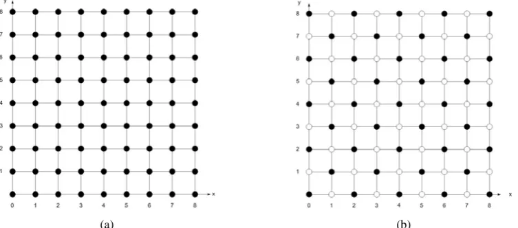
(a) (b)

Figure 1. (a) All nodes will be considered in full-sweep iteration case. (b) For half-sweep iteration, only black (black dot) nodes are considered.

[image:3.595.113.490.65.231.2]

(a) (b)

Figure 2: The stencil of (a) full-sweep and (b) half-sweep cases, respectively.

The half-sweep iteration technique was first applied in robotics application in [19]. Essentially, the half-sweep iteration is based on the five points rotated finite difference approximation equation, which was first introduced by Abdullah [21] for solving problem in Eq. (1). The main characteristic of such iterative method is to reduce the computational complexity by considering only half of the total node points.

The stencil for full-sweep case is shown in Figure 2 (a), whereas Figure 2 (b) shows the stencil of half-sweep iteration technique. The half-sweep approximation equation is actually a rotated 45° of Eq. (3) as shown in Eq. (4).

U_i−1,j−1+U_i+1,j−1+U_i−1,j+1+U_i+1,j+1−4U_i,j =0 (4)

When SOR is embedded to Eq. (4) by adding a weighted parameter, see Young [20],[21], the implementation of the half-sweep iteration can be shown as

k j i k j i k j i k j i k j i k j

i U U U U U

U_, 1 ( _{1, 1 1, 1 1, 1 1, 1}) (1 ) _,

4 ω

ω _{+ + + + −}

= − − + − − + + +

+ ₍₅₎

Furthermore, Red-Black ordering strategy [23],[4] is applied to the half-sweep iteration technique to demonstrate the effectiveness of HSSOR-RB in solving path planning

problem. With Red-Black ordering, first loop starting at the even row of bottom left, then going up to next even row and so on, see Eq. (6). Then when all points on even rows are finished, do the computation for points on odd rows, again starting on odd row of bottom left. This particular ordering is very interesting, since it is completely parallel within the red points (points on even rows) and within the black points (points on odd row).

Computation of red points at domain

Ω

R

n i U U U U U U k j i k j i k j i k j i k j i k j i ,... 6 , 4 , 2 , ) 1 ( ) (

4 1, 1 1, 1 1, 1 1, 1 ,

1 , = − + + + + = − − + − − + + +

+ ω _ω

(6)

Computation of black points at domain

Ω

B

1 ,... 7 , 5 , 3 , ) 1 ( ) (

4 1, 1 1, 1 1, 1 1, 1 ,

1 , − = − + + + + = − − + − − + + + + n i U U U U U U k j i k j i k j i k j i k j i k j i ω ω (7)

[image:3.595.124.474.292.436.2]

(a) (b)

(c) (d)

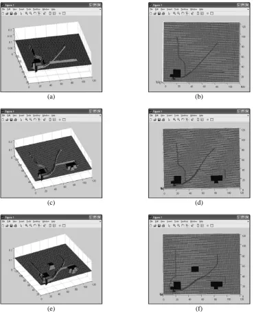
[image:4.595.116.487.59.514.2]

(e) (f)

[image:4.595.61.535.590.689.2]

Figure 3: The paths generated with HSSOR iterative method. (a) and (b) One obstacle. (c) and (d) Two obstacles. (e) and (f) Three obstacles.

Table 1. Performance comparison of the several numerical techniques with varying number of obstacles.

FSGS (one obstacle)

FSGS-RB (one obstacle)

HSGS-RB (one obstacle)

HSSOR-RB (one obstacle)

HSSOR -RB (two obstacles)

HSSOR-RB (three obstacles) Number of

iterations 19,716 19,067 8,436 546 477 296

Maximum

error 9.999

-10

9.993-10 9.986-10 9.712-10 9.959-10 9.880-10

Period in

B. Simulation

The experiment considered a static environment that consists of a goal point, three starting points and varying number of obstacles (Box shape object, L and T shape objects). Initially, the outer boundaries (walls) and obstacles were fixed with high temperature values. Goal point was set to very low temperature. All other free spaces were set to zero temperature value. Then, the iteration process was run on Intel Core 2 Duo CPU running at 1.83GHz speed with 1GB of RAM to compute temperature values numerically at all points in the environment. The iteration process was terminated when there was no more changes in temperature values, where it converged to zero error solution. The highest precision of solution was required to avoid flat area that would cause the path generation algorithm to fail to reach the goal point. A major improvement in this study was discovered by relaxing the requirement of zero error solution as reported in earlier work [19]. Instead of setting maximum error to zero, the value was set to very small value of 1.0-10. It was found that by setting such very small tolerance, it was sufficient to avoid flat area in the resulting temperature values. Moreover, the setting had reduced the number of iteration tremendously, thus produced the generated paths very rapidly.

Table 1 shows the number of iterations, maximum error and period in seconds required to compute all temperature values in the environment for all numerical techniques compared in the experiment. For HSSOR-RB method, several weight values were tested to observe its effect in reducing the number of iterations, but ω=1.9 were chosen for its best performance. Clearly, HSSOR-RB iterative method proved to be very fast compared to the previous methods. Note that the speed of computation gets faster as the number of obstacles increases. This is due to less number of nodes to be computed, since nodes occupied by obstacles are ignored during computation.

Once the temperature values were obtained, the path was generated by performing steepest descent search from start points to goal point. In all experiments, all three paths were successfully generated. The process of generating the paths was very fast. From the current point, the algorithm simply picked the lowest temperature value from its four neighbourhood points. This process continues, until the generated path reached the goal point.

Figure 3 (a) and (b) shows the generated paths in one-obstacle environment, Figure 3 (c) and (d) for two-obstacle environment and Figure 3 (e) and (f) for three-obstacle environment. As shown in Figure 3, the boundaries and obstacles temperature values are raised up for visualization purpose. The lowest temperature indicates the goal point. All other areas are almost flat due to very small difference in temperature values, except for the area close to the goal point. Note that FSGS-RB and HSGS-RB iterative methods produced very similar visual to one-obstacle HSSOR-RB method as shown in Figure 3 (a) and (b).

The environment shown in Figure 3 represents an area of approximately 120x120 units. As shown in Figure 3, the three generated paths started from three different locations. In the experiment, all of them successfully ended at the same goal point with different obstacles setting, although they

were differed in speed to reach the goal point. The generated paths successfully avoided the various shapes of obstacles in the environment. The somewhat jagged nature of the paths was due to the fact that no interpolation was performed here. Interpolation of the gradient would provide smoother paths.

I. CONCLUSION

The experiment in this study shows that solving robot path planning problem using numerical techniques are indeed very attractive and feasible due to the recent advanced and new found techniques, as well as the availability of fast machine nowadays. In this paper, it is shown that error tolerance can be set to a very small value to speed up the convergence rate. Such setting is sufficient to avoid flat areas that will cause the generated path to fail to reach the goal point. As shown in Table 1, the HSSOR-RB iterative method proved to be very fast (less than two seconds) compared to previous FSGS-RB and HSGS-RB methods.

REFERENCES

[1] Connolly, C. I., & Gruppen, R. 1993. On the applications of harmonic

functions to robotics. Journal of Robotic Systems, 10(7): 931–946

[2] Saudi, A. and Sulaiman, J. 2009. Efficient Weighted Block Iterative

Method for Robot Path Planning Using Harmonic Functions. In proc. of the 2nd International Conference on Control, Instrumentation and Mechatronic Engineering (CIM09), Malacca, Malaysia, June 2-3, 2009

[3] Saudi, A. and Sulaiman, J. 2009. Block Iterative Method for Robot

Path Planning. The 2nd Seminar on Engineering and Information Technology (SEIT2009), Kota Kinabalu, Malaysia, July 8-9, 2009

[4] Ibrahim, A. 1993. The Study of the Iterative Solution Of Boundary

Value Problem by the Finite Difference Methods. PhD Thesis. Universiti Kebangsaan Malaysia

[5] Khatib, O. 1985. Real time obstacle avoidance for manipulators and

mobile robots. IEEE Transactions on Robotics and Automation 1:500–505

[6] Koditschek, D. E. 1987. Exact robot navigation by means of potential

functions: Some topological considerations. Proceedings of the IEEE International Conference on Robotics and Automation: 1-6

[7] Connolly, C. I., Burns, J. B., & Weiss, R. 1990. Path planning using

Laplace’s equation. Proceedings of the IEEE International Conference on Robotics and Automation: 2102–2106

[8] Akishita, S., Kawamura, S., & Hayashi, K. 1990. Laplace potential for

moving obstacle avoidance and approach of a mobile robot. Japan-USA Symposium on flexible automation, A Pacific rim conference: 139–142

[9] Sasaki, S. 1998. A Practical Computational Technique for Mobile

Robot Navigation. Proceedings of the IEEE International Conference on Control Applications: 1323-1327

[10] Abdullah, A.R.: The Four Point Explicit Decoupled Group (EDG)

Method: A Fast Poisson Solver. International Journal of Computer Mathematics 38, 61–70 (1991)

[11] Daily, R., & Bevly, D.M. 2008. Harmonic Potential Field Path

Planning for High Speed Vehicles. In the proceeding of American Control Conference, Seattle, June 11-13, 4609-4614

[12] Ibrahim, A., Abdullah, A.R. 1995. Solving the two-dimensional

diffusion equation by the four point explicit decoupled group (EDG) iterative method. International Journal Computer Mathematics, 58 (1995) 253-256

[13] Yousif, W. S., Evans, D. J. : Explicit De-coupled Group iterative

methods and their implementations. Parallel Algorithms and Applications, 7 (2001) 53-71

[14] Abdullah, A.R., Ali, N.H.M.: A Comparative Study of Parallel

Strategies for the Solution of Elliptic PDE’s. Parallel Algorithms and Applications, 10 (1996) 93–103

[15] Sulaiman, J., Hasan, M.K., and Othman, M. The Half-Sweep Iterative

Alternating Decomposition Explicit (HSIADE) Method for Diffusion Equation. CIS 2004, LNCS 3314, pp. 57–63, 2004. Springer-Verlag Berlin Heidelberg, 2004

[16] Willms, A.R. and Simon X.Y. 2008. IEEE Transactions on Systems,

Real-Time Robot Path Planning via a Distance-Propagating Dynamic System with Obstacle Clearance

[17] Jan. G.E., Chang, K.Y., and Parberry I. 2008. Optimal Path Planning

for Mobile Robot Navigation. IEEE/ASME Transactions on Mechatronics, Vol. 13, No. 4, August 2008, pages 451-460

[18] Bhattacharya, P. and Gavrilova, M.L. 2008. Roadmap-Based Path

Planning - Using the Voronoi Diagram for a Clearance-Based Shortest Path. IEEE Robotics & Automation Magazine, Volume 15, Issue 2, June 2008. Page(s):58 – 66

[19] Saudi, A. and Sulaiman, J. 2009. Half-Sweep Gauss-Seidel (HSGS)

Iterative Method for Robot Path Planning. The 3rd Int. Conf. on Informatics and Technology (Informatics09), Kuala Lumpur, 27-28 Oct 2009

[20] Young, D. M. 1954. Iterative Methods for solving Partial Difference

Equations of Elliptic Type, Trans. Amer. Math. Soc.,76: 92-111

[21] Young, D.M. 1971. Iterative solution of large linear systems. London:

Academic Press.

[22] J. Sulaiman, M. Othman, and M.K. Hasan. 2009. Nine Point-EDGSOR

Iterative Method for the Finite Element Solution of 2D Poisson Equations. O. Gervasi et al. (Eds.): ICCSA 2009, Part I, LNCS 5592, pp. 764–774, 2009. Springer-Verlag Berlin Heidelberg

[23] Sulaiman, J., Othman, M. & Hasan., M.K, “The Red-Black Half-Sweep

iteration to solve first order hyperbolic equations”, Proceedings of the

2nd _{International Conference on Research and Education in}