Hyperspectral Image Classification based on
Dimensionality Reduction and Swarm Optimization
Approach
Murinto
Departement of Informatics Engineering Universitas Ahmad Dahlan
Yogyakarta
Dewi Pramudia Ismi
Departement of Informatics Engineering Universitas Ahmad Dahlan
Yogyakarta
Erik Iman H. U.
Departement of Informatics Engineering
Universitas Teknologi Yogyakarta
ABSTRACT
Hyperspectral images have high dimensions, making it difficult to determine accurate and efficient image segmentation algorithms. Dimension reduction data is done to overcome these problems. In this paper we use Discriminant independent component analysis (DICA). The accuracy and efficiency of the segmentation algorithm used will affect final results of image classification. In this paper a new method of multilevel thresholding is introduced for segmentation of hyperspectral images. A method of swarm optimization approach, namely Darwinian Particle Swarm Optimization (DPSO) is used to find n-1 optimal m-level threshold on a given image. A new classification image approach based on Darwinian particle swarm optimization (DPSO) and support vector machine (SVM) is used in this paper. The method introduced in this paper is compared to existing approach. The results showed that the proposed method was better than the standard SVM in terms of classification accuracy namely average accuracy (AA), overall accuracy (OA and Kappa index (K).
General Terms
Evolutionary algorithms, Segmentation, Classification
Keywords
Darwinian Particle Swarm Optimization, Hyperspectral Image, Support Vector Machine
1.
INTRODUCTION
Hyperspectral imaging also known as spectroscopy imaging is a technique that is well known among several fields of research, especially in remote sensing satellite. This technique relates to measurement, analysis and interpretation of spectral obtained from a scene or a particular object in short, medium and long waves through an airborne or satellite sensor. The concept of hyperspectral imaging was first raised by the Jer Propulsion Laboratory Airborne Visible Infrared Imaging Spectrometer (AVIRIS), where a system the Airborne Imaging Spectrometer (AIS) was built to explain this technology [1].
Image classification plays an important role in the analysis image. Some examples of image classification applications include land cover mapping, forest management, regional development, etc. One of the things that are important in classification is obtaining high accuracy. Accuracy plays a very important role in a variety of applications, including in the remote sensing field. One way to improve accuracy is use sequential spatial-spectral information [2]. Methods for finding spatial information among others are morphological
filters [3], watershed methods [4], and Markov random fields [5]. While another way to improve accuracy results by involving spatial information is to use the spatial structure that will be displayed in image segmentation.
Image segmentation is a procedure that can be used to modify the accuracy of classification maps. Several methods for multispectral and hyperspectral image segmentation have been introduced in some literature. Some of these methods are based on a method of merging regions, where adjacent segmented areas are combined with others according to their homogeneity criteria. One simple and very well known method for image segmentation is thresholding. Various types of optimal thresholding methods have been introduced in the literature [6] [7]. One strategy for finding the optimal threshold set is to take into account exhaustive search. The search method commonly used is based on the Otsu’s criteria [8]. Searching to find the optimal n-1 threshold involves evaluating fitness for combination of threshold and L is the intensity level in each component. Therefore, this method is not desirable if it is viewed in terms of computing time. Alternatively, the problem of determining n-1 optimal threshold for thresholding n-level imagery can be formulated as a multidimensional optimization problem. To solve this problem, several biologically inspired algorithms have been explored in image segmentation [8].
One segmentation method based on the threshold is the Darwinian Particle Swarm Optimization (DPSO) which can overcome trapping of local optima commonly experienced by traditional Particle Swarm Optimization (PSO). In this paper, a new spectral-spatial classification approach is introduced to improve the classification accuracy of hyperspectral images. First, the input image will be reduced in dimension by using Discriminant independent component analysis (DICA), the results will be segmented by DPSO. In the end, segmented images will be classified using support vector machine (SVM). The result form image segmentation and spectral classification is combined by using majority vote (MV) approach.
2.
MATERIAL AND METHODOLOGY
Flow chart of method in this paper is shown in Figure-2. Dimensional reduction of data was carried out by using Discriminant independent component analysis (DICA). The segmentation multilevel thresholding method based on DPSO, and spectral information classified by SVM.2.1
Dataset Image
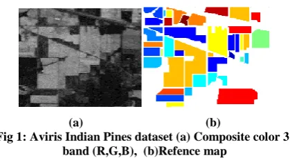
Aviris Indian Pines Data: image used to research is Indian Pines hyperspectral. Image obtained from Aviris sensor that flew over the north western Indiana area in 1992. This image has a size of its spectral resolution of 145 x 145 pixels. Where in this image consists of 220 spectral bands (Noise already omitted) [9]. Ground truth Indian pines hyperspectral image consists of 16 classes: Alfafa, corn no-till, corn-min till, corn, grass-pasture, grass-trees, grass-mowed, hay-windowed, oats, soybean-no till, soybean-min till, soybean-cleam, wheat, woods, building-tress-drive, stone-steel-tower. Figure 1 is depicts Aviris Indian Pines dataset and its reference map.
[image:2.595.62.272.272.388.2](a) (b)
Fig 1: Aviris Indian Pines dataset (a) Composite color 3-band (R,G,B), (b)Refence map
2.2
Discriminant Independent Component
Analysis
In the Discriminant independent component analysis (DICA) method, multivariate data with lower dimensions and independent features are obtained through Negentropy maximization. In DICA, the Fisher criterion and the sum of marginal negentropy independent features are extracted by maximizing simultaneously. Negentropy is a statistical estimate of non-Gaussian random variables. An approach of marginal negentropy can be written as an equation (1).
(1)
In the equation (1), and represented non quadratic function odd and even. There are some general elections for a random vector with symmetrical distribution (normal):
(2)
(3)
(4) Maximization of the marginal quantity of Negentropy with covariance unit can be obtained through the Lagrange equation in the following form:
(5)
The features can be obtained by maximizing the target function in equation (5). The optimization problem that maximizes the function of criteria from the classification and negentropy performance of the independent features extracted
simultaneously can be defined by an Lagrange equation in the following form:
(6) k is constant. is a function to measure efficient classification from features y given C, and same with equation (5).
2.3
Multilevel Thresholding Segmentation
Using DPSO
Multilevel segmentation techniques provide an efficient way to image analysis. The problem faced is usually the automatic selection of an optimal n-level threshold. Threshold can be found using the Otsu’s method [10], which can maximize variance between classes. Pixels of an image are represented in the L gray level. Number of pixels at level i as , the total number of pixels denoted through . The gray level histogram is normalized and is considered probability distribution equation written in the equation (1).
, , (7)
Images are divided into classes and by a threshold at level k in bi-level thresholding problem. is pixels with levels and is pixels with levels . Probabilites of class occurences and mean class levels can be written as equatuons (8) and (9) respectivelyt. While the average total level of the image can be write as equation (10).
(8)
(9)
(10)
Two relation can be written as equation (11) for several choices of k.
, (11)
Furthermore, the objective function of the Otsu method can be defined as equation (12).
Maximim (12) Otsu’s method can be extended to multilevel thresholding problems. It is assumed that there is a threshold, which divides the image into m + 1 class: for for
and for . Kemudian fungsi dari metode Otsu dituliskan kembali sebagai persamaan ( 13). Maximies
(13)
One method used to perform segmentation processes is to use the thresholding method. Threshold image thresholding T partitioning an image I into parts of a particular region based on the value of T itself. Suppose there is an L level of intensity in each RGB component of an image, and these levels are within the range of values (0, 1, 2, L-1), then it can be defined in equation (14).
, , (14) Where is intensity, K is image components,
. N is total numbers pixels in image. is number of pixels for intensity level i correspondens with component K. While total average (mean) is mean that combinated from every image component as a equation (15).
from 2-level thresholding can extended to find n-level thresholding where is n-1 level threshold ,
. Image can be written as equation function (16).
(16) Where si x and y are widht (W) and length (H) image pixels write as dwith inetensity level Lin each RGB components. In this situation pixels of the image will be divided into n classes which is represents multiple objects or certain features on a particular object. The method to get the optimal threshold is by maximizing the variance between classes through equation (17).
, (17)
Where is j represented specific class so that and are probability of occurence (event) and mean from class j. Probability of occurence and classes given as equations (18).
(18)
While the mean of each class calculated using equation (19).
(19)
This n-level thresholding optimization problem is reduced to a search optimization problem for the threshold which maximizes 3 objective functions (i.e. fitness function) of each RGB component written in the form of equation (20).
(20)
The original PSO algorithm was introduced by Eberhart and Kennedy in 1995 [11]. Basically, the PSO comes from the advantages of the swarm intelligence concept, which is a collection of behavioral systems from simple agents that integrate locally with its environment which makes coherence global functional patterns. Based on the concept of PSO inheritance, DPSO was derived. Certain algorithms can work well on one problem but may fail in another. If an algorithm can be designed to adapt to the fitness function, adjust itself to the fitness landscape, a stronger algorithm with wider application, without the need for special engineering problems
will result. In finding a better natural selection model using the PSO algorithm, Darwinian Particle Swarm Optimization (DPSO) was introduced by Tillet et al. [12].
A few simple rules are followed to remove flocks, remove particles, and spawn new flocks and new particles: i) when the herd population is below the minimum, the flock is removed; and ii) the worst performing particles in the herd are removed when the maximum number of steps (counter search) without increasing the fitness function is achieved. After deletion of particles, instead of being set to zero, the counter is reset to the value close to the threshold number, according to the equation (21).
(21)
Where is as the number of particles removed from swarm (flocks) during periods where there is no improvement in fitness.
2.4
Support Vector Machine
Increasing number of features given to the input of a classifier with a given threshold will be affect classification accuracy decreases. This event is called Hughes phenomenon. The approach taken to overcome this problem consists of 4 approaches [13]: 1).Regularization sample of covariance matrix. The approach uses a normal multivariate probability density (Gaussian) model, usually widely used in remote sensing data, 2).Adaptation of statistical estimates through the exploitation of classified, 3).Feature extraction, 4).Spectral analysis class model.
The concept of support vector machine(SVM) mathematically is given as follows: Given a sample training data
, where each sample has d input and a label class with one of two values . All hyperplane in are parameterized through normal non-zero (w) vector which in reality is an orthogonal vector to the hyperplane and constant (b), written in equation (22).
(22) Where x is point in the same space as the hyperplane. Supposes there are two hyperplane that canonical (normalization) given through the equation (23).
(23) The distance from given points is calculates use equation (24).
(24) Support vector is defined as points on the canonical hyperplane. SVM non linear in input space, still in form of linear feature space. Space is obtained through kernel functions. The decision function can be simplified into a form:
(25)
The kernel that is usually used in SVM is in the form of: Kernel polynomial :
(26) 1. Kernel Radial Basis Function (RBF) :
2.5
Evaluation of Classification Result
In this paper evaluation of classification result that will be carried out by measuring classification accuracy (classification accuracy assessment). The results of spatial comparison from evaluation pixel are displayed in error matrix or confusion matrix. The results of comparison are measured using statistical test Kappa index (K). After image classification obtained, the results of the classification are measured and assessed to get feedback as an evaluation material for improved concept developed.Data accuracy test is done by comparing two maps, where one map comes from remote sensing analysis (map tested) and the other is a map that comes from another source. The second map is used as reference map, and is assumed to have correct information. The truth of accuracy test results is done by using a confusion matrix that identifies not only errors for a category but also misclassification between categories. From information in the confusion matrix, it can be learned that classification deviations in form of excess number of pixels from other classes or emissions (omission) and lack of pixels in each class or commission.
A confusion matrix is a table where each column represents a value in a prediction class, while each row represents a value in the actual class. The accuracy of classification can be further calculated from the confusion matrix. The overall accuracy (OA) is the percentage of pixels that are correctly classified. Specific class accuracy or procedure accuracy (CA) is percentage of pixels that are correctly classified for a given class. Average accuracy (AA) is the mean of certain class accuracy for all classes. The Kappa coefficient is a percentage of conformity, i.e. pixels that are correctly classified, is justified through the expected amount of conformity purely through change.
3.
EXPERIMENT RESULT AND
ANALYSIS
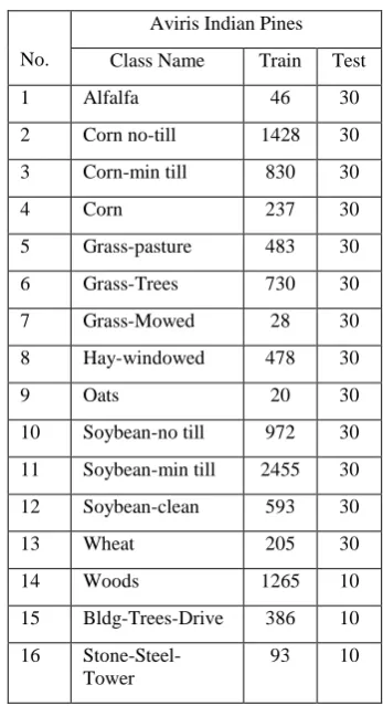
[image:4.595.340.514.94.414.2]Hyperspectral image used in this paper is produce by Airborne Visible /Infrared Imaging Spectrometer (AVIRIS). This sensor operates in visible, near and mid-infrared spectrum, which has a wavelength range from 0.4 to 2.4 . The sensor system has 224 data channels, 4 spectrometers, where each spectral bad is estimated to be 10nm wide. The spatial resolution is 20m. The Indian Pines image was obtained from AVIRIS sensors above Northwestern Indiana in 1992. The original image was 145 x 145 pixels. The image contains 202 spectral bands (after being reduced by spectral bands containing noise and water absorption), the image consists of only 190 spectral bands used in this study. This image contains 16 corresponding classes: Alfalfa, corn no-till, corn-min till, corn, grass-pasture, grass-trees, grass-mowed, oats, soybean-no till, soybean-min till, soybean-clean, building-trees-drive, stone-steel-tower. In Table 1 we can show the number of training and testing sample Aviris Indian Pines dataset.
Table 1: Training-testing Samples for Aviris Indian Pines Hyperspectral Image Data Sets
No.
Aviris Indian Pines Class Name Train Test
1 Alfalfa 46 30
2 Corn no-till 1428 30
3 Corn-min till 830 30
4 Corn 237 30
5 Grass-pasture 483 30
6 Grass-Trees 730 30
7 Grass-Mowed 28 30
8 Hay-windowed 478 30
9 Oats 20 30
10 Soybean-no till 972 30 11 Soybean-min till 2455 30 12 Soybean-clean 593 30
13 Wheat 205 30
14 Woods 1265 10
15 Bldg-Trees-Drive 386 10
16 Stone-Steel-Tower
93 10
.
The first, input image is reduced dimensions by using Discriminant independent component analysis (DICA). The first three independent components (IC’s) are selected since they contain 95 percent of the total variance in dataset. The classification method proposed in this paper is based on Darwinian particle swarm optimization (DPSO) and support vector machine (SVM).
In Figure 2 a classification system of spectral-spatial hyperspectral images is shown which is built on a supervised learning scheme. Training samples and tests are taken from a set of image data following a particular sampling strategy. After image processing involving spectral-spatial operations, feature extraction steps combine spectral and spatial information to explore the most discriminatory features in different classes. The extracted feature is used to train a classifier that minimizes errors in the training set.
From Figure 2 can be seen that the Aviris Indian Pines image prior to the classification process was reduced in dimensions. The approach used is to use Discriminant independent component analysis (DICA) [14] [15]. The first three independent components (IC's) are retained for use in the next process. The output of this step is then segmented using the DPSO method. In this paper, the hyperspectral image segmentation method uses Darwinian particle swarm optimization (DPSO).
Table 2: Parameter Initialization of DPSO
Parameter DPSO
Iteration numbers 150 Population number 50
C1 0.5
C2 0.5
Vmax -4
Vmin 4
Xmax 0
Xmin -
Population Maximal - Population Minimal -
Numbers of Swarm -
Min Swarm -
Max Swarm -
Stagnancy -
[image:5.595.79.255.83.343.2]CPU processing time of the data set used in this paper was tested on DPSO algorithms respectively for thresholding levels of 8, 10 and 12, 14. The average CPU processing time was obtained from 20 runs. The results are shown in Table 3. In the level 8, 10, 12, and 14 value of average CPU processing time are 5.5201, 5.5382, 5.9245, and 5.9710, respectively.
Table 3: Average CPU Processing Time
Level DPSO
8 5.5201
10 5.5382
12 5.9245
14 5.9710
The final results of segmentation using DPSO and spectral classification using support vector machines (SVM) combined with using majority vote (MV). A combination of segmentation map and classification based on pixels is done in this study. It is an approach where classification based on pixels is based on spectral information and image segmentation is displayed separately, then the results of segmentation and classification are combined using a previously defined fusion rule. This combination approach is called Majority Vote (MV) [16].
The approach of the majority vote the steps are as follows: 1. Classification based on pixels which are based
solely on pixel spectral information and segmentation is done independently. In supervised cases it usually uses SVM for classification based on pixels.
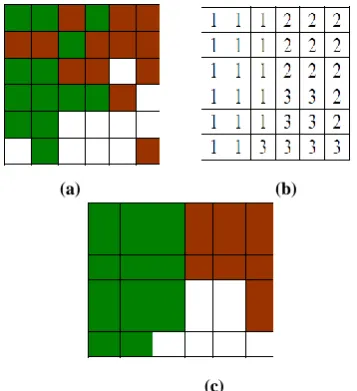
2. In each region on the segmentation map, all pixels are entered into the class with the highest frequency among these regions. In Figure 3 show example of MV.
(a) (b)
(c)
Figure 3 : Example of majority vote implementation for spectal-spatial based classification. (a) Classification map;
(b) segmentation map; (c) Majority vote in a region segmentation
Figure 4 shows the image of Aviris Indian Pines RGB, an example of data dimension reduction using Discriminant independent component analysis (DICA) and segmentation methods using level-12 DPSO method. In this paper
(a) (b) (c ) Figure 4: Aviris Indian Pines data set: (a) RGB Image (b) the first independent components (c) level 12 thresholding
using DPSO
In Figure 5 illustrates the standard SVM classification map and the proposed classification method with segmentation using DPSO level 8, 10, 12, and 14.
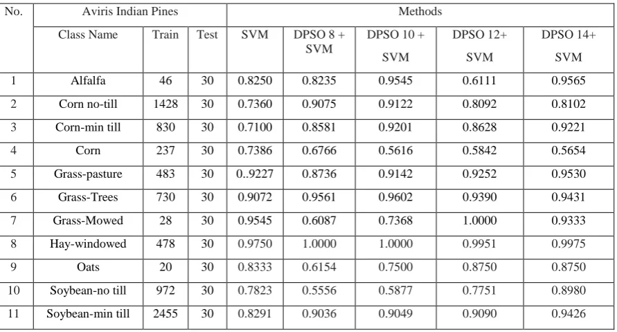
The output of SVM presents much pixel noise which can reduce the results of classification accuracy. The results showed in Table 4 that overall accuracy (OA) for SVM and new methods with levels 8.10, 12, and 14 are 0.8262, 0.8514, 0.8669, 0.8712, and 0.9059, respectively. Average accuracy (AA) value of SVM and four new methods are 0.8450, 0.8389, 0.8594, 0.8583, and 0.8978, respectively. Kappa index value of SVM and four new methods are 0.8014, 0.8300, 0.8474, 0.8521, and 0.8916, respectively.
[image:5.595.318.538.364.474.2] [image:5.595.106.222.427.523.2](a) (b) (c)
[image:6.595.67.269.72.248.2](d) (e)
Figure 5: Classification Map Aviris Indian Pines data set (a-e) of the SVM with-10 fold cross validation and the
classification method with 8,10,12, and 14 level segmentation by DPSO
4.
CONCLUSIONS
In this paper a data dimension reduction technique using Discriminant independent component analysis (DICA) and image segmentation using Darwinian particle swarm optimization (DPSO) is proposed for grouping pixels in hyperspectral images. The experimental results show that the DPSO is robust especially for higher levels of segmentation. The efficiency of image segmentation using DPSO used is then combined with the support vector machines (SVM) method on image classification using a majority vote (MV). The results showed that using the proposed method of SVM + DPSO with levels 8,10,12 and 14 there was an increase in the Kappa index of 2.86%, 4.60%, 5.07%, 9.02% respectively.
5.
ACKNOWLEDGMENTS
The researchers expressed gratitude to DP2M-RISTEKDIKTI who has funded this research with National Strategic Research Institution (PSNI) scheme 2018
Spectral Classification (SVM) Spatial Information (DPSO)
Spectral-Spatial information (MV)
[image:6.595.55.470.282.492.2]Result Map Classification DICA
Figure 2: Flowchart of DPSO and SVM classification approach
Table 4: Classification Accuracy Aviris Indian Pines Hyperspectral Image Data Sets
No. Aviris Indian Pines Methods
Class Name Train Test SVM DPSO 8 +
SVM
DPSO 10 +
SVM
DPSO 12+
SVM
DPSO 14+
SVM
1 Alfalfa 46 30 0.8250 0.8235 0.9545 0.6111 0.9565
2 Corn no-till 1428 30 0.7360 0.9075 0.9122 0.8092 0.8102
3 Corn-min till 830 30 0.7100 0.8581 0.9201 0.8628 0.9221
4 Corn 237 30 0.7386 0.6766 0.5616 0.5842 0.5654
5 Grass-pasture 483 30 0..9227 0.8736 0.9142 0.9252 0.9530
6 Grass-Trees 730 30 0.9072 0.9561 0.9602 0.9390 0.9431
7 Grass-Mowed 28 30 0.9545 0.6087 0.7368 1.0000 0.9333
8 Hay-windowed 478 30 0.9750 1.0000 1.0000 0.9951 0.9975
9 Oats 20 30 0.8333 0.6154 0.7500 0.8750 0.8750
10 Soybean-no till 972 30 0.7823 0.5556 0.5877 0.7751 0.8980
[image:6.595.78.524.523.763.2]12 Soybean-clean 593 30 0.7335 0.8757 0.8462 0.8452 0.9670
13 Wheat 205 30 0.9144 0.9928 0.9784 0.9857 0.9653
14 Woods 1265 10 0.9146 0.9965 0.9948 0.9789 0.9702
15 Bldg-Trees-Drive 386 10 0.7296 0.8392 0.8107 0.6802 0.8413
16 Stone-Steel-Tower 93 10 0.9868 0.9400 0.9184 0.9565 0.8846
OA 0.8262 0.8514 0.8669 0.8712 0.9059
AA 0.8450 0.8389 0.8594 0.8583 0.8978
Kappa 0.8014 0.8300 0.8474 0.8521 0.8916
6.
REFERENCES
[1] [Green, R.O., Eastwood, M.L and Sarture, C.M. et al.” Imaging spectroscopy and the airborne visible/infrared imaging spectrometer (AVIRIS)”, Remote Sensing of Environment, 65, 227-248.
[2] Ghamisi, P., Benediktsson, J. A., & Ulfarsson, M. O, “The spectral-spatial classification of hyperspectral images based on Hidden Markov Random Field and its Expectation-Maximization” In Geoscience and Remote Sensing Symposium (IGARSS), 2013 IEEE International (pp. 1107-1110).
[3] Fauvel, M., Benediktsson, J. A., Chanussot, J., & Sveinsson, J. R, “Spectral and spatial classification of hyperspectral data using SVMs and morphological Profiles”, IEEE Transactions on Geoscience and Remote Sensing, 2008, 46(11), 3804-3814.
[4] Tarabalka, Yuliya, Jón Atli Benediktsson, and Jocelyn Chanussot, “Spectral–spatial classification of hyperspectral imagery based on partitional clustering techniques”, IEEE Transactions on Geoscience and Remote Sensing 47.8. 2009: 2973-2987.
[5] Tarabalka, Y., Fauvel, M., Chanussot, J., & Benediktsson, J. A, “SVM-and MRF-based method for accurate classification of hyperspectral images”, IEEE Geoscience and Remote Sensing Letters, 7(4), 2010, pp:736-740.
[6] Mishra, D., Bose, I., De, U. C., & Pradhan, B, “A multilevel image thresholding using particle swarm optimizatiol”, International Journal of Engineering and Technology, 6(6), 2014, pp:1204-1211.
[7] Oliva, D., Cuevas, E., Pajares, G., Zaldivar, D., & Perez-Cisneros, M. 2013. Multilevel thresholding segmentation based on harmony search optimization.Journal of Applied Mathematics.
[8] Suresh, S., & Lal, S, “Multilevel thresholding based on Chaotic Darwinian Particle Swarm Optimization for segmentation of satellite images”, Applied Soft Computing, 55, 2017, 503-522.
[9] AVIRIS Dataset. [cited 2016 June 1].Available fromftp://ftp.ecn.purdue.edu/biehl/MultiSpec/92AV3C .tif.zip, 2002.
[10] Otsu, N, “A threshold selection method from gray-level histograms. IEEE transactions on systems, man, and cybernetics”, 1979, 9(1), 62-66.
[11] Eberhart, R., & Kennedy, J, “A new optimizer using particle swarm theory”, In Micro Machine and Human Science, 1995. MHS’95. Proceedings of the Sixth International Symposium on, 1995, (pp. 39-43). [12] Tillett, J., Rao, T., Sahin, F., & Rao, R, “Darwinian
particle swarm optimization”, 2005.
[13] Melgani, F. and Bruzzone, L, “Classification of Hyperspectral Remote Sensing Images with Support Vector Machines”, IEEE Transactions on Geoscience and Remote Sensing, 42,2004, 1778-179.
[14] Murinto and Nur Rochmah Dyah PA, “Dimensionality Reduction using Hybrid Support Vector Machine and Discriminant Independent Component Analysis for Hyperspectral Image”, International Journal of Advanced Computer Science and Applications(IJACSA), 2017, 8(11).
[15] Dhir, Chandra S, and Soo-Young Lee,”Discriminant independent component analysis”. IEEE transcations on neural networks 22.6 (2005):845-857.