Statistical Inference for Pareto Distribution based on Progressive Type I Hybrid Censoring Scheme

(1)

Statistical Inference for Pareto Distribution based on

Progressive Type-I Hybrid Censoring Scheme

M. M. Mohie El-Din

Department of Mathematics

Faculty of Science Al-Azhar University

Egypt

A. R. Shafay

Faculty of Science Fayoum University

Egypt

M. Nagy

Egypt

A. Gamal

Egypt

ABSTRACT

In this paper, the maximum likelihood and Bayesian estimations are developed based on progressive Type-I hybrid censored sample from the Pareto distribution. The Bayesian estimators for the unknown parameters are computed using the squared error loss function. Also, the point and interval Bayesian predictions for the unobserved failures from the same sample and that from the future sample are derived. Moreover, a Monte Carlo simulation study is carried out to compare the performance of the maximum likelihood and the Bayesian estimators. Finally, numerical example is presented for illustrating all the inferential procedures developed here.

Keywords

Bayesian estimation, Bayesian prediction, Pareto distribution, Maximum likelihood estimation, progressive hybrid censoring sample

1. INTRODUCTION

In reliability analysis, experiments are often terminated before all units on test fail based on cost and time considerations. In such cases, failure information is available and only partial information is available on all units that have not failed. Such data are called censored data. There are several forms of censored data. Two commonly used right censoring schemes are the Type-I and Type-II censoring, wherein the test terminates, respectively, at a pre-determined time T and upon observing certain number of failures. If n is the number identical units on a life-testing experiment, in the Type-I censoring scheme the experiment is terminated when a pre-fixed censoring timeT is reached. In the Type-II censoring scheme, the experiment gets terminated when a pre-specified numberm≤nof failures is observed. The mixture of Type-I and Type-II censoring schemes is known as a hybrid censoring scheme.

Progressive II censoring scheme is a generalization of Type-II censoring scheme, wheren−munits are withdrawn from the life-test at different time points (rather than all at the timeXm:n). When the first failure is observed,R1of then−1surviving units are randomly selected and removed. At the second observed failure,

R2 of then−R1−2surviving units are randomly selected and removed. The experiment finally terminates at the time of themth

failure when all remainingRm=n−R1−. . .−Rm−1−m surviv-ing units are removed. The censorsurviv-ing numbers{Ri, i= 1, .., m} are prefixed. The resultingmordered values which are obtained from this type of censoring are referred to as progressively Type-II right censored order statistics. Several authors have studied progressive Type-II censoring and properties of order statistics arising from such a progressively censored life-test. Some key references are Aggarwala and Balakrishnan [1], Cramer and Iliopoulos [2], Raqab et al. [3], Mohie El-Din and Shafay [4], and Balakrishnan and Cohen [5].

The disadvantages of the progressive Type-II censoring scheme are that the time of the experiment can be very long if the units are highly reliable. Therefore, Kundu and Joarder in [6] and Childs et al. in [7] proposed a progressive Type-I hybrid censoring scheme (HCS), in this life-testing the experiment is terminated at time

min{Xm:m:n, T}, whereT ∈(0,∞)pre-fixed in advance. Under progressive Type-I HCS, the time on experiment will be no more thanT. Some recent studies on progressive hybrid censored sample have been carried out by many authors including Lin et al. [8], Lin and Huang. [9], and Hemmati and Khorram [10].

In this paper, the underlying distribution is assumed to be the Pareto distribution which introduced by Pareto in [11] as a model for the distribution of income, with the probability density function (PDF) and cumulative distribution function (CDF) given by

f(x|α, σ) = α σ

σ

x (α+1)

, x≥σ, (1)

and

F(x|α, σ) = 1−σ x

α

. (2)

whereα >0andσ >0.

In recent years, its models in several different forms have been studied by many authors including Davis and Feldstein[12], Cohen and Whitten[13], and Grimshaw [14].

(2)

distribution is derived in Section 5. Finally, in Section 6, a Monte Carlo simulation study is carried out to compare the performance of the ML and the Bayesian estimates, for illustrating all the inferential methods developed here, numerical example is then presented.

2. THE MODEL DESCRIPTION

The progressive Type-I HCS can be described as follow: Supposen

identical items are put to test and the lifetime distributions of then

items are denoted byX1, X2, ..., Xn. The integerm < nis fixed at the beginnig of the experiment, andR= (R1, R2, ..., Rm)are

mpre-fixed integers satisfyingn=m+R1+. . .+Rm. The time pointT is also fixed beforehand. At the time of first failureX1:m:n,

R1of the remaining units are randomly removed. Similarly, at the time of the second failure X2:m:n, R2of the remaining units are removed and so on. If themth_failure_X

m:m:noccurs before the time pointT, the experiment stops at the time pointXm:m:n. On the other hand, supposemth _{failure does not occur before time} pointT and onlykfailures occur before the time pointT, where

0≤k < m; then, at the time pointT all the remainingR∗

τ units are removed and the experiment terminates at the time pointT .

Note thatR∗

τ = m

P

i=k+1

(Ri+ 1).(see Fig. 1).

𝑅𝑚

. . .

𝑅𝑡∗

𝑇∗_{= 𝑇}

𝑅1 𝑅2

𝑋1:𝑚:𝑛

𝑅𝑚−1

𝑋2:𝑚:𝑛 𝑋𝑚−1:𝑚:𝑛 𝑇

𝑅1 𝑅2

𝑋1:𝑚:𝑛

𝑅𝑘

[image:2.595.316.557.73.236.2]

𝑋2:𝑚:𝑛 𝑋𝑘:𝑚:𝑛

Fig. 1. Schematic representation of progressive Type-I hybrid censoring scheme Case I: 𝑿𝒎:𝒎:𝒏< 𝑻

Case II: 𝑻 < 𝑿𝒎:𝒎:𝒏

. . . . . .

𝑇∗= 𝑋𝑚−1:𝑚:𝑛

Therefore, in the presence of progressively Type-I HCS, one of the following types of observations is found:

(1) Suppose that the mth _{failure occurs before} _T_{, then the} experiment terminates atT and{X1:m:n < ... < Xk:m:n} are observed.

(2) Suppose that the mth _{failure occurs before} _T,_{then the} experiment terminates at Xm:m:n and {X1:m:n < ... <

Xm:m:n}are observed.

Given a progressively Type-I HCS, the joint density function for the different cases are as follows:

fX(x) = "_D

Y

i=1 m

X

j=i

R∗_j+ 1 #

D

Y

i=1

f(xi:D:n)

_¯ F(xi:D:n)

Ri_¯ F(T)R∗τ

,

(3)

where

D=

k ifXk:m:n≤T < Xm:m:n,

m ifXm:m:n< T, (4)

withR∗

τ is the number of surviving units that are removed atT, given by

R∗τ =





 n−k−

k

P

j=1

Rj ifXk:m:n≤T < Xm:m:n,

0 ifXm:m:n< T,

(5)

and

x=

(x1:m:n, ..., xk:m:n) if, Xk:m:n≤T < Xm:m:n

(x1:m:n, ..., xm:m:n) ifXm:m:n< T, (6)

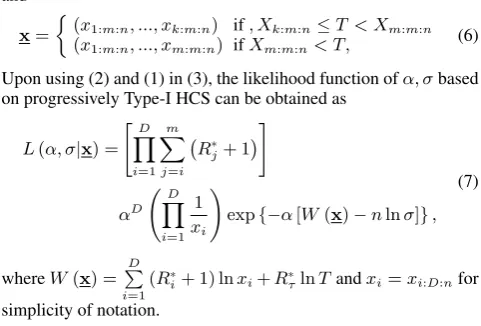
Upon using (2) and (1) in (3), the likelihood function ofα, σbased on progressively Type-I HCS can be obtained as

L(α, σ|x) = "D

Y

i=1 m

X

j=i

R∗j+ 1

#

αD D

Y

i=1

1 xi

!

exp{−α[W(x)−nlnσ]},

(7)

whereW(x) =

D

P

i=1

(R∗

i+ 1) lnxi+R∗τlnTandxi=xi:D:nfor simplicity of notation.

3. THE ML AND BAYESIAN ESTIMATIONS It is clear that the likelihood function is monotone increasing function inσ, so its maximum valueσ_bM L will be attained at the minimum valuex1:m:mofσ. From (7), The log-likelihood function of(α, σ)is given by

ln [L(α, σ|x)] =const.+Dlnα−α[W(x)−nlnσ], (8)

to maximize relative toα, differentiate (8) with respect toαand solve the equation

∂ln [L(α, σ|x)] ∂α = 0,

so the ML estimatorαbM Lofαis obtained as

b αM L=

D

W(x)−nlnx1:m:m

. (9)

For the Bayesian estimations, under the assumption that both parametersαandσare unknown, the joint prior density function ofαandσ, which was suggested by Lwin in [15] and generalized by Arnold and Press in [16], is considered. The generalized Lwin prior or the power-gamma prior is given by

π(α, σ) ∝ αa_σ−1_exp[_−α_(ln_g₋_b_ln_σ_)]_{, α >}₀_,₀_{< σ < h,} (10) wherea, b, g, hare positive constants andhb_{< g}_.

Upon combining (7) and (10), given progressively Type-I HCS, the posterior density function ofα, σis obtained as

π∗(α, σ|x) =L(α, σ|x)π(α, σ)/ Z

L(α, σ|x)π(α, σ)dαdσ

=I−1_αD+a_σ−1_exp_{−α_[_W₍_x₎₋₍_n₊_b_{) ln}_σ_{+ ln}_g_]_}_, (11)

where

I =

x0

Z

0

∞ Z

0

αD+a_σ−1_exp_{−α_[_W₍_x₎₋₍_n₊_b_{) ln}_σ_{+ ln}_g_]_}_dαdσ

= Γ(D+a)

n+b [W(x)−(n+b) lnx0+ lng] −(D+a)

, (12)

(3)

density function, given by

b αB =

x0 Z 0 ∞ Z 0

απ∗(α, σ|x)dαdσ

= D+a

W(x)−(n+b) lnx0+ lng

, (13)

and the Bayesian estimator ofσunder the squared error loss function is obtained as

b σB =

x0 Z 0 ∞ Z 0

σπ∗(α, σ|x)dαdσ

= I−1 x0

∞

Z

0

αD+a

α(n+b) + 1exp{−α[W(x)−(n+b) lnx0+ lng]}dα

= I

−1_x 0

(n+b)[W(x)−(n+b) lnx0+ lng]

−(D+a)

× ∞ Z

0

tD+a_e−t

t+ [W(x)−(n+b) lnx0+ lng]/(n+b)

dt

= x0

Γ(D+a)Φ

D+a,[W(x)−(n+b) lnx0+ lng]

(n+b)

, (14)

where

Φ (x, y) =

∞ Z

0

tx_e−t

t+ydt.

A partial tabulation ofψ(x, y) = (y/Γ(x))Φ (x−1, y)has been provided by Arnold and Press in [16].

4. ONE-SAMPLE BAYESIAN PREDICTION Forρ= 1,2, ..., R∗

j, letXρ:R∗

j denote theρ

th_{order statistic out of}

R∗jremoved units at stagej. Then, the conditional density function ofXρ:R∗_j, given the observed progressively Type-I HCS, is given, see Basak et al. [17], by

fXρ:R∗

j

(x|x) = R ∗ j! (ρ−1)!(R∗

j−ρ)!

[F(x)−F(xj)]ρ −1

[1−F(x)]R∗

j−ρ_f₍_x₎

[1−F(xj)] R∗

j

, x > xj,

(15) where

j=

1, ..., m ifXm:m:n< T,

1, ..., k, τ ifXk:m:n≤T < Xm:m:n,

withxτ=T.

By using (2) and (1) in (15), given Type-I PHCS, the conditional density function ofXρ:R∗_j is then given as follows:

fX_ρ_:_R∗

j

(x|x) =

ρ−1

X

q=0

C1q

α

xexp{−α[ηq(lnx−lnxj)]}, x > xj,

(16)

where C1q=

(−1)q₍ρ−1

q )R∗j!

(ρ−1)!(R∗_j−ρ)! and ηq=q+R

∗

j−ρ+ 1 for

q= 0, ..., ρ−1.Upon combining (11) and (16), the Bayesian predictive density function ofXρ:R∗

j, given progressively Type-I

HCS, is obtained as

f∗

X_ρ_:_R∗

j

(x|x)

= x0 Z 0 ∞ Z 0

fX_ρ_:_R∗

j

(x|x)π∗(α, σ|x)dαdσ

=I−

1_Γ(_D₊_a_{+ 1)}

(n+b) ρ−1 X

q=0 Cq

x [W(x)−(n+b) lnx0+ lng+ηq(lnx−lnxj)]

−(D+a+1) .

(17)

The Bayesian predictive survival function of Xρ:R∗

j, given

progressively Type-I HCS, is given as

¯ F_X∗

ρ:R∗_j(t|x)

=

∞ Z

t

f_X∗

ρ:R∗_j(x|x)dx

=I−

1 Γ(D+a) (n+b)

ρ−1 X

q=0 Cq

ηq [W(x)−(n+b) lnx0+ lng+ηq(lnt−lnxj)]

−(D+a) .

(18)

The Bayesian point predictor ofXρ:R∗

j under the squared error loss

function is the mean of the predictive density, given by

b Xρ:R∗_j =

∞ Z

0

xfX∗_ρ_:_R∗

j

(x|x)dx, (19)

wheref∗₍_x|_x₎

is given as in (17).

The Bayesian predictive bounds of 100(1−γ)% two-sided equi-tailed (ET) interval forXρ:R∗

j can be obtained by solving the

following two equations:

¯ F_X∗

ρ:R∗_j(LET|x) =

γ

2 and F¯

∗

X_ρ_:_R∗

j

(UET|x) = 1−

γ 2,

(20) whereF¯∗₍_t|_x₎

is given as in (18), andLET andUET denote the lower and upper bounds, respectively. On the other hand, for the highest posterior density (HPD) method, the following two equations need to be solved:

¯ F_X∗

ρ:R∗_j(LHP D|x)−

¯ F_X∗

ρ:R∗_j(UHP D|x) = 1−γ

and

f_X∗

ρ:R∗_j(LHP D|x)−f

∗

X_ρ_:_R∗

j

(UHP D|x) = 0,

wheref∗(x|x)is as in (17), andLHP DandUHP Ddenote the HPD lower and upper bounds, respectively.

5. TWO-SAMPLE BAYESIAN PREDICTION Let Y1:`:N≤ Y2:`:N≤ . . .≤ Y`:`:N be a future independent progressive Type-II censored sample from the same population with censoring scheme S = (S1, ... , S`). In this section, a general procedure for deriving the point and interval predictions forYs:`:N,1≤s≤ `, based on the observed progressively Type-I HCS, is developed. The marginal density function ofYs:`:N is given by Balakrishnan et al. in [18] as

fYs:`:N(ys) =c(N, s)

s−1

X

q=0

cq,s−1[1−F(ys)]

Mq,s−1_f₍_y

(4)

where1≤s≤ρ,

c(N, s) =N(N−S1−1)...(N−S1...−Ss−1+ 1),

Mq,s=N−S1−...−Ss−q−1−s+q+ 1, andcq,s−1= (−1)q

("

q

Q

u=1 s−q+u−1

P

υ=s−q

(Sυ+ 1)

# s−q−1

Q

u=1 s−q−1

P

υ=u

(Sυ+ 1)

)−1 .

Upon substituting (2) and (1) in (21), the marginal density function ofYs:`:Nis then obtained as

fYs:`:N(ys) =c(N, s)

s−1 X

q=0 cq,s−1

α ysexp

n

−αhMq,slnys σ

io , ys>0.

(22) Upon combining (11) and (22), given progressively Type-I HCS, the Bayesian predictive density function ofYs:`:Nis obtained as

f_Y∗

s:`:N(ys|x) =

( f∗

1Ys:`:N(ys|x), 0< ys≤x0,

f∗

2Ys:`:N(ys|x), ys> x0,

(23)

where

f ∗1Ys:`:N(ys|x)

= ys Z 0 ∞ Z 0

fYs:`:N(ys|x)π

∗

(α, σ|x)dαdσ

= I−1_Γ(_D₊_a_{+ 1)}_c₍_{N, s}₎ s−1

X

q=0

cq,s−1

(n+b+Mq,s)ys

×[W(x)−(n+b) lnys+ lng]

−(D+a+1)

, (24)

and

f ∗₂_Y

s:`:N(ys|x)

= x0 Z 0 ∞ Z 0

fYs:`:N(ys|x)π

∗

(α, σ|x)dαdσ

= I−1Γ(D+a+ 1)c(N, s)

s−1

X

q=0

cq,s−1

(n+b+Mq,s)ys

×[W(x)−(n+b+Mq,s) lnx0+Mq,slnys+ lng]

−(D+a+1)

.

(25)

From (23), the predictive survival function of Ys:`:N, given progressively Type-I HCS, is obtained as

¯

FY∗_s_:_`_:_N(t|x) =

( ¯ F∗

1Ys:`:N(t|x), 0< t≤x0,

¯ F∗

2Ys:`:N(t|x), t > x0,

(26)

where

¯ F ∗₁_Y

s:`:N(t|x)

=

x0

Z

t

f1∗Ys:`:N(ys|x)dys+

∞ Z

x0

f2∗Ys:`:N(ys|x)dys

= I−1Γ(D+a)c(N, s)

s−1

X

q=0

cq,s−1

(n+b) (n+b+Mq,s)Mq,s

×n(n+b+Mq,s) [W(x)−(n+b) lnx0+ lng]

−(D+a)

−Mq,s[W(x)−(n+b) lnt+ lng]

−(D+a)o

, (27)

and

¯

F ∗2Ys:`:N(t|x)

=

∞ Z

t

f₂∗_Y

s:`:N(ys|x)dys

= I−1Γ(D+a)c(N, s)

s−1

X

q=0

cq,s−1

Mq,s(n+b+Mq,s)

×[W(x)−(n+b+Mq,s) lnx0+Mq,slnt+ lng]

−(D+a)

.

(28)

The Bayesian point predictor ofYs:`:N,1 ≤ s ≤ m, under the squared error loss function is the mean of the predictive density, given by

b Ys:`:N=

∞ Z

0

ysfY∗s:`:N(ys|x)dys, (29)

wheref∗

Ys:`:N(ys|x)is given as in (23).

6. NUMERICAL RESULTS

Before progressing further, how to generate the progressively Type-I HCS, for a given setn,m,R1, R2, ..., RmandT, is described. The following transformation, suggested in Balakrishnan and Aggarwala [19], is used:

Z1=nX1:m:n

Z2=(n−R1−1)(X2:m:n-X1:m:n) .

. .

Zm=(n−R1−1)(Xm:m:n-Xm−1:m:n).

It is known that ifXi’s are i.i.d. , then the spacingsZi’s are also i.i.d. random variables. Then it follows that

X1:m:n=n1Z1

X2:m:n=n−R11−1Z2+ 1 nZ1 .

. .

Xm:m:n=n−R1−...−1Rm−1−m−1Zm+...+ 1 nZ1.

Thus, the progressively Type-I HCS can be easily generated as follows. If Xm:m:n < T, then the progressive Type-I hybrid censored sample X1:m:n,...,Xm:m:n is obtained. If T <

Xm:m:n, then the progressive Type-I hybrid censored sample

X1:m:n, ..., Xk:m:nis obtained whereXk:m:n< T < Xk+1:m:n.

6.1 Monte Carlo Simulation

In this section, a Monte Carlo simulation study is carried out to compare the performance of the ML and the Bayesian estimates under different sampling schemes. Different values forn, mand

(5)

(1) Scheme 1:Ri= 2(n−m)

m ifiis odd andRi= 0ifiis even. (2) Scheme 2:Ri=2(n

−m)

m ifiis even andRi= 0ifi is odd. (3) Scheme 3:R1=R2=...=Rm−1= 1andRm=n−2m+

1.

All Bayesian results are computed based on two different choices of the hyperparameters(a, b, g, h), namely,

(1) Informative prior(IP) : a= 1.78,b= 0.33,g= 3.48and

h= 11.40.

(2) Noninformative prior(N IP) : a = −1,b = 0,g = 1and

h=∞.

6.2 Numerical example

In this numerical example, a progressive Type-I hybrid censored sample from a sample of size n = 25 is generated. Suppose

m= 15andR = (1,0,0,0,0,3,0,0,0,3,0,0,0,0,3), then the following generated data: 6.0034, 6.0641, 6.2204, 6.2437, 6.2638, 6.2939, 6.3944, 6.3949, 6.5048, 6.5280, 6.7037, 6.7572, 7.9157, 8.5940, and 9.1067 are obtained. Different values fork and T

are considered to obtaine the following three different progressive Type-I HCS:

(1) Scheme 1: SupposeT = 6.500, sinceT < X15:15:25, then the experiment would have terminated atX8:15:25, withR∗

τ=

13, and the following data: 6.0034, 6.0641, 6.2204, 6.2437, 6.2638, 6.2939, 6.3944, and 6.3949 are obtained.

(2) Scheme 2: SupposeT = 10, sinceX15:15:25 < T, then the experiment would have terminated atX15:15:25, with R∗

τ =

0, and the following data: 6.0034, 6.0641, 6.2204, 6.2437, 6.2638, 6.2939, 6.3944, 6.3949, 6.5048, 6.5280, 6.7037, 6.7572, 7.9157, 8.5940, and 9.1067 are obtained.

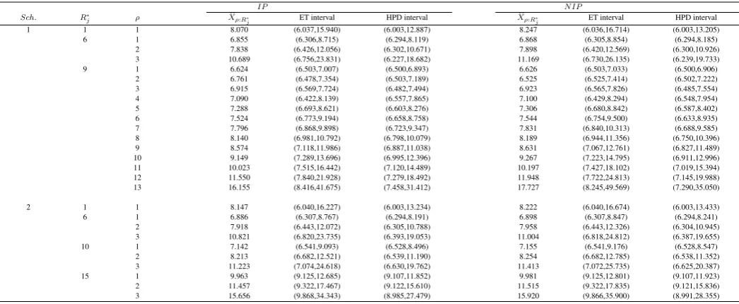
These data are assumed to have come from the Pareto distribution with α and σ are unknown. Based on the above generated progressive Type-I hybrid censored sample, Table 3 presents the point predictor and95%ET and HPD prediction intervals ofXρ:R∗

j

and Table 4 presents the point predictor and95% ET and HPD prediction intervals ofYs:`:Nfrom the future progressive censored sample of size `= 10 from a sample of sizeN = 20 with progressive censoring scheme S= (2,0,2,0,2,0,2,0,2,0 ).

6.3 Conclusions and discussion

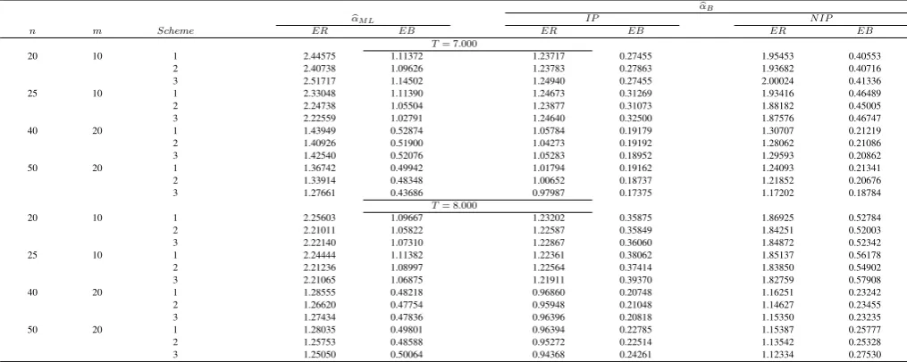
From Tables 1 and 2, it can be seen that the performance of the ML estimators is quite close to that of the Bayesian estimators based noninformative priors, as expected. Thus, if no prior information on the unknown parameters is found, then it is always better to use the ML rather than the Bayesian estimators, because the Bayesian estimators are computationally more sensitive. Also, the Bayesian method with informative priors is the best method for estimation under all different censoring schemes. Moreover, mean-squared error decreases whennandmincrease.

From the results in Tables 3 and 4, it can be seen that the point predictor of mean is between the upper and lower bounds of the prediction intervals. Also, the lower bounds are relatively insensitive while the upper bounds are more sensitive. Moreover, a comparison of the results for the informative priors with the corresponding ones for non-informative priors reveals that the former produce more precise results. Finally, the HPD prediction intervals seem to be more precise than the ET prediction intervals. In this paper, the maximum likelihood and Bayesian estimators are derived for the two unknown parameters of the Pareto distribution

based on progressive Type-I hybrid censored sample. Even though many results of interest in estimation and prediction have been addressed in this paper, there are many problems in this direction are open further study. One possible problem that will be of interest is to use the progressive Type-I hybrid censoring scheme for developing the estimation and prediction problems for some other continuous distribution such as (1) Weibull distribution, (2) Burr Type-XII distribution, (3) Inverted exponential distribution, and (4) Generalized inverted exponential distribution. Another possible problem that will be of interest is to consider the estimation and prediction problems based on some other forms of censoring schemes such as (1) Progressive Type-II hybrid censoring scheme, (2) Adaptive progressively Type-I censoring scheme, and (3) Unified hybrid censoring scheme.

7. REFERENCES

[1] R. Aggarwala, N. Balakrishnan,(1998). Some properties of progressive censored order statistics from arbitrary and uniform distributions with applications to inference and simulation.J.of Stat. Plan. and Infer.70,35-49.

[2] E. Cramer, G. Iliopoulos,(2010). Adaptive progressive Type-II ensoring,Test.19,342-358.

[3] M. Z. Raqab, A. Asgharzadeh, R. Valiollahi, (2010). Prediction for Pareto distribution based on progressively Type-II censored samples, Comput. Stat. – Data Anal. 54, 1732-1743.

[4] M. M. Mohie El-Din, A. R. Shafay, (2013). One-and two-sample Bayesian prediction intervals based on progressively Type-II censored data,Stat. Papers.54,287-307.

[5] N. Balakrishnan, A. C. Cohen, (2014).Order statistics -inference: estimation methods. Elsevier .

[6] D. Kundu, A. Joarder, (2006). Analysis of Type - II progressively hybrid censored data, Comput. Stat.– Data Anal.50,2509-2528.

[7] A. Childs, B. Chandrasekar, N. Balakrishnan,(2008). Exact likelihood inference for an exponential parameter under progressive hybrid censoring schemes, In Stat. models and methods for biomedical and tech. Sys.319-330.

[8] C.T. Lin, C.C. Chou, Y.L. Huang,(2012). Inference for the Weibull distribution with progressive hybrid censoring, Comput. Stat. – Data Anal.56,451-467.

[9] C.T. Lin, Y.L. Huang,(2012). On progressive hybrid censored exponential distribution, J.of Stat. Comput. and Simul. 82, 689-709.

[10] F. Hemmati, E. Khorram,(2013). Statistical analysis of the log-normal distribution under Type-II progressive hybrid censoring schemes,Commun. in Stat.-Simul. and Comput.42, 52-75.

[11] V. Pareto,(1897).Cours d’Economie Politique, Rouge et Cie, Paris.

[12] H.T. Davis, M.L. Feldstein,(1979). The generalized Pareto law as a model for progressively censored survival data, Biometrika,66,299-306.

[13] A.C. Cohen, B.J. Whitten,(1988). Parameter Estimation in Reliability and Life Span Models, Marcel Dekker, Inc, New York .

(6)

[15] T. Lwin,(1972). Estimation of the tail of the Paretian law, Scandinavian Actuarial J.55, 170-178.

[16] B.C. Arnold, S. J. Press, (1989). Bayesian estimation and prediction for Pareto data.J.of the American Stat. Association, 84,1079-1084.

[17] I. Basak, P. Basak, N. Balakrishnan, (2006). On some predictors of times to failure of censored items in progressively censored samples.Comput. stat. – Data Anal, 50,1313-1337.

[18] N. Balakrishnan, A. Childs, B. Chandrasekar,(2002). An efficient computational method for moments of order statistics under progressive censoring. Stat. – Probability Letters, 60,359-365.

(7)

[image:7.595.51.559.125.328.2]

Table 1. The values of EB and ER of the ML and Bayesian estimates forα.

b

αB

b

αM L IP N IP

n m Scheme ER EB ER EB ER EB

T= 7.000

20 10 1 2.44575 1.11372 1.23717 0.27455 1.95453 0.40553

2 2.40738 1.09626 1.23783 0.27863 1.93682 0.40716

3 2.51717 1.14502 1.24940 0.27455 2.00024 0.41336

25 10 1 2.33048 1.11390 1.24673 0.31269 1.93416 0.46489

2 2.24738 1.05504 1.23877 0.31073 1.88182 0.45005

3 2.22559 1.02791 1.24640 0.32500 1.87576 0.46747

40 20 1 1.43949 0.52874 1.05784 0.19179 1.30707 0.21219

2 1.40926 0.51900 1.04273 0.19192 1.28062 0.21086

3 1.42540 0.52076 1.05283 0.18952 1.29593 0.20862

50 20 1 1.36742 0.49942 1.01794 0.19162 1.24093 0.21341

2 1.33914 0.48348 1.00652 0.18737 1.21852 0.20676

3 1.27661 0.43686 0.97987 0.17375 1.17202 0.18784

T= 8.000

20 10 1 2.25603 1.09667 1.23202 0.35875 1.86925 0.52784

2 2.21011 1.05822 1.22587 0.35849 1.84251 0.52003

3 2.22140 1.07310 1.22867 0.36060 1.84872 0.52342

25 10 1 2.24444 1.11382 1.22361 0.38062 1.85137 0.56178

2 2.21236 1.08997 1.22564 0.37414 1.83850 0.54902

3 2.21065 1.06875 1.21911 0.39370 1.82759 0.57908

40 20 1 1.28555 0.48218 0.96860 0.20748 1.16251 0.23242

2 1.26620 0.47754 0.95948 0.21048 1.14627 0.23455

3 1.27434 0.47836 0.96396 0.20818 1.15350 0.23235

50 20 1 1.28035 0.49801 0.96394 0.22785 1.15387 0.25777

2 1.25753 0.48588 0.95272 0.22514 1.13542 0.25328

3 1.25050 0.50064 0.94368 0.24261 1.12334 0.27530

Table 2. The values of EB and ER of the ML and Bayesian estimates forσ.

b

σB

b

σM L IP N IP

n m Scheme ER EB ER EB ER EB

T= 7.000

20 10 1 0.10765 0.07313 0.08297 0.01201 0.11201 0.03022

2 0.10765 0.07313 0.08317 0.01124 0.11029 0.02731

3 0.10765 0.07313 0.08307 0.01155 0.11054 0.02837

25 10 1 0.08571 0.05835 0.06561 0.00822 0.07406 0.01734

2 0.08571 0.05835 0.06544 0.00772 0.07169 0.01564

3 0.08571 0.05835 0.06555 0.00706 0.07107 0.01397

40 20 1 0.05456 0.03856 0.03956 0.00177 0.04058 0.00385

2 0.05456 0.03856 0.03950 0.00163 0.04045 0.00360

3 0.05456 0.03856 0.03952 0.00174 0.04050 0.00378

50 20 1 0.04356 0.03081 0.03132 0.00112 0.03183 0.00237

2 0.04356 0.03081 0.03133 0.00107 0.03182 0.00228

3 0.04356 0.03081 0.03127 0.00092 0.03167 0.00199

T= 8.000

20 10 1 0.10765 0.07313 0.08074 0.00705 0.08476 0.01404

2 0.10765 0.07313 0.08064 0.00660 0.08413 0.01296

3 0.10765 0.07313 0.08070 0.00676 0.08441 0.01338

25 10 1 0.08571 0.05835 0.06424 0.00530 0.06697 0.00982

2 0.08571 0.05835 0.06439 0.00509 0.06686 0.00920

3 0.08571 0.05835 0.06416 0.00448 0.06614 0.00797

40 20 1 0.05456 0.03856 0.03904 0.00051 0.03856 0.00149

2 0.05456 0.03856 0.03900 0.00039 0.03932 0.00166

3 0.05456 0.03856 0.03898 0.00045 0.03931 0.00158

50 20 1 0.04356 0.03081 0.03110 0.00016 0.03133 0.00089

2 0.04356 0.03081 0.03109 0.00022 0.03132 0.00098

[image:7.595.47.560.442.646.2]

(8)

[image:8.595.43.566.134.349.2]

Table 3. Bayesian point predictor and95%ET and HPD prediction intervals forXρ:R∗_j.

IP N IP

Sch. R∗

j ρ Xbρ:R∗

j ET interval HPD interval Xbρ:R∗j ET interval HPD interval

1 1 1 8.070 (6.037,15.940) (6.003,12.887) 8.247 (6.036,16.714) (6.003,13.205)

6 1 6.855 (6.306,8.715) (6.294,8.119) 6.868 (6.305,8.854) (6.294,8.185)

2 7.838 (6.426,12.056) (6.302,10.671) 7.898 (6.420,12.569) (6.300,10.926)

3 10.689 (6.756,23.831) (6.227,18.682) 11.169 (6.730,26.135) (6.239,19.733)

9 1 6.624 (6.503,7.007) (6.500,6.893) 6.626 (6.503,7.033) (6.500,6.906)

2 6.761 (6.478,7.354) (6.503,7.189) 6.525 (6.525,7.414) (6.502,7.222)

3 6.915 (6.569,7.724) (6.482,7.494) 6.923 (6.565,7.826) (6.485,7.554)

4 7.090 (6.422,8.139) (6.557,7.865) 7.100 (6.429,8.294) (6.548,7.954)

5 7.288 (6.693,8.621) (6.603,8.276) 7.306 (6.680,8.842) (6.587,8.402)

6 7.524 (6.773,9.194) (6.658,8.758) 7.544 (6.754,9.500) (6.633,8.935)

7 7.796 (6.868,9.898) (6.723,9.347) 7.831 (6.840,10.313) (6.688,9.585)

8 8.140 (6.981,10.792) (6.798,10.079) 8.189 (6.944,11.356) (6.750,10.396)

9 8.574 (7.118,11.986) (6.887,11.038) 8.631 (7.067,12.761) (6.827,11.489)

10 9.149 (7.289,13.696) (6.995,12.396) 9.267 (7.223,14.795) (6.911,12.996)

11 10.023 (7.515,16.442) (7.120,14.489) 10.197 (7.427,18.102) (7.019,15.394)

12 11.550 (7.840,21.928) (7.279,18.492) 11.948 (7.722,24.813) (7.145,19.988)

13 16.155 (8.416,41.675) (7.458,31.412) 17.727 (8.245,49.569) (7.290,35.050)

2 1 1 8.147 (6.040,16.227) (6.003,13.234) 8.222 (6.040,16.674) (6.003,13.433)

6 1 6.886 (6.307,8.767) (6.294,8.191) 6.898 (6.307,8.847) (6.294,8.241)

2 7.918 (6.443,12.072) (6.305,10.788) 7.958 (6.443,12.326) (6.304,10.945)

3 10.821 (6.820,23.735) (6.393,19.053) 11.004 (6.818,24.812) (6.387,19.655)

10 1 7.142 (6.541,9.093) (6.528,8.496) 7.155 (6.541,9.176) (6.528,8.547)

2 8.213 (6.682,12.521) (6.539,11.190) 8.254 (6.682,12.785) (6.538,11.352)

3 11.223 (7.074,24.618) (6.630,19.762) 11.413 (7.072,25.735) (6.625,20.387)

15 1 9.963 (9.125,12.685) (9.107,11.852) 9.981 (9.125,12.801) (9.107,11.923)

2 11.457 (9.322,17.467) (9.122,15.610) 11.515 (9.322,17.835) (9.121,15.836)

3 15.656 (9.868,34.343) (8.985,27.479) 15.920 (9.866,35.900) (8.991,28.355)

Table 4. Bayesian point predictor and95%ET and HPD prediction intervals forYs:`:N.

IP N IP

Scheme s Ybs:N ET interval HPD interval Ybs:N ET interval HPD interval

1 1 6.020 (5.834,6.247) (5.823,6.235) 6.019 (5.826,6.255) (5.814,6.242)

2 6.107 (5.892,6.462) (5.864,6.418) 6.108 (5.889,6.487) (5.857,6.435)

3 6.201 (5.949,6.677) (5.908,6.601) 6.204 (5.947,6.724) (5.901,6.631)

4 6.320 (6.007,6.956) (5.954,6.835) 6.325 (6.005,7.034) (5.946,6.882)

5 6.452 (6.063,7.263) (6.001,7.091) 6.459 (6.059,7.378) (5.991,7.159)

6 6.633 (6.131,7.712) (6.051,7.460) 6.644 (6.122,7.883) (6.038,7.560)

7 6.844 (6.207,8.238) (6.100,7.891) 6.862 (6.192,8.482) (6.082,8.033)

8 7.203 (6.315,9.242) (6.152,8.690) 7.232 (6.292,9.621) (6.127,8.908)

9 7.686 (6.454,10.643) (6.203,9.792) 7.737 (6.419,11.234) (6.170,10.126)

10 10.452 (6.799,22.781) (6.250,17.985) 10.785 (6.738,25.128) (6.208,19.092)

2 1 6.020 (5.827,6.255) (5.816,6.243) 6.020 (5.821,6.261) (5.810,6.248)

2 6.113 (5.886,6.467) (5.860,6.429) 6.114 (5.881,6.480) (5.472,6.440)

3 6.212 (5.944,6.676) (5.907,6.613) 2.215 (5.941,6.699) (5.902,6.630)

4 6.338 (6.007,6.944) (5.958,6.846) 6.343 (4.006,6.980) (5.953,6.872)

5 6.477 (6.071,7.236) (6.012,7.098) 6.485 (6.070,7.287) (6.007,7.135)

6 6.668 (6.149,7.664) (6.070,7.462) 6.680 (6.147,7.739) (6.065,7.515)

7 6.891 (6.238,8.163) (6.130,7.886) 6.908 (6.234,8.266) (6.124,7.958)

8 7.268 (6.366,9.125) (6.197,8.677) 7.295 (6.362,9.284) (6.188,8.786)

9 7.776 (6.530,10.456) (6.267,9.763) 7.816 (6.524,10.701) (6.255,9.927)

[image:8.595.57.553.475.638.2]