Implicitly Defined Neural Networks for Sequence Labeling

(1)

Proceedings of the 55th Annual Meeting of the Association for Computational Linguistics (Short Papers), pages 172–177 Vancouver, Canada, July 30 - August 4, 2017. c2017 Association for Computational Linguistics

Implicitly-Defined Neural Networks for Sequence Labeling

∗

Michaeel Kazi, Brian Thompson

MIT Lincoln Laboratory

244 Wood St, Lexington, MA, 02420, USA

{first.last_}@ll.mit.edu

Abstract

In this work, we propose a novel, implicitly-defined neural network archi-tecture and describe a method to compute its components. The proposed architec-ture forgoes the causality assumption used to formulate recurrent neural networks and instead couples the hidden states of the network, allowing improvement on prob-lems with complex, long-distance depen-dencies. Initial experiments demonstrate the new architecture outperforms both the Stanford Parser and baseline bidirectional networks on the Penn Treebank Part-of-Speech tagging task and a baseline bidi-rectional network on an additional artifi-cial random biased walk task.

1 Introduction

Feedforward neural networks were designed to ap-proximate and interpolate functions. Recurrent Neural Networks (RNNs) were developed to pre-dict sequences. RNNs can be ‘unwrapped’ and thought of as very deep feedforward networks, with weights shared between each layer. Com-putation proceeds one step at a time, like the tra-jectory of an ordinary differential equation when solving an initial value problem. The path of an initial value problem depends only on the current state and the current value of the forcing func-tion. In a RNN, the analogy is the current hidden state and the current input sequence. However, in certain applications in natural language process-ing, especially those with long-distance dependen-cies or where grammar matters, sequence

predic-∗_{This work is sponsored by the Air Force Research} Lab-oratory under Air Force contract FA-8721-05-C-0002. Opin-ions, interpretatOpin-ions, conclusions and recommendations are those of the authors and are not necessarily endorsed by the United States Government.

tion may be better thought of as a boundary value problem. Changing the value of the forcing func-tion (analogously, of an input sequence element) at any point in the sequence will affect the val-ues everywhere else. The bidirectional recurrent network (Schuster and Paliwal,1997) attempts to addresses this problem by creating a network with two recurrent hidden states – one that progresses in the forward direction and one that progresses in the reverse. This allows information to flow in both directions, but each state can only consider information from one direction. In practice many algorithms require more than two passes through the data to determine an answer. We provide a novel mechanism that is able to process informa-tion in both direcinforma-tions, with the motivainforma-tion being a program which iterates over itself until conver-gence.

1.1 Related Work

Bidirectional, long-distance dependencies in se-quences have been an issue as long as there have been NLP tasks, and there are many approaches to dealing with them.

Hidden Markov models (HMMs) (Rabiner, 1989) have been used extensively for sequence-based tasks, but they rely on the Markov assump-tion – that a hidden variable changes its state based only on its current state and observables. In finding maximum likelihood state sequences, the Forward-Backward algorithm can take into ac-count the entire set of observables, but the under-lying model is still local.

In recent years, popularity of the Long Short-Term Memory (LSTM) (Hochreiter and Schmid-huber,1997) and variants such as the Gated Recur-rent Unit (GRU) (Cho et al.,2014) has soared, as they enable RNNs to process long sequences with-out the problem of vanishing or exploding gradi-ents (Pascanu et al.,2013). However, these models

(2)

only allow for information/gradient information to flow in the forward direction.

The Bidirectional LSTM (b-LSTM) (Graves and Schmidhuber, 2005), a natural extension of (Schuster and Paliwal, 1997), incorporates past and future hidden states via two separate recurrent networks, allowing information/gradients to flow in both directions of a sequence. This is a very loose coupling, however.

In contrast to these methods, our work goes a step further, fully coupling the entire sequences of hidden states of an RNN. Our work is similar to (Finkel et al.,2005), which augments a CRF with long-distance constraints. However, our work dif-fers in that we extend an RNN and uses Netwon-Krylov (Knoll and Keyes,2004) instead of Gibbs Sampling.

2 The Implicit Neural Network (INN) 2.1 Traditional Recurrent Neural Networks

A typical recurrent neural network has a (pos-sibly transformed) input sequence [ξ1, ξ2, . . . , ξn]

and initial statehsand iteratively produces future

states:

h1 = f(ξ1, hs)

h2 = f(ξ2, h1) . . .

hn = f(ξn, hn−1)

[image:2.595.315.512.491.726.2]

The LSTM, GRU, and related variants follow this formula, with different choices for the state transition function. Computation proceeds learly, with each next state depending only on in-puts and previously computed hidden states.

Figure 1: Traditional RNN structure.

2.2 Proposed Architecture

In this work, we relax this assumption by allowing ht =f(ξt, ht−1, ht+1)1. This leads to an implicit set of equations for the entire sequence of hidden states, which can be thought of as a single tensor

1_{A wider stencil can also be used, e.g.}_f_(h

t−2, ht−1, . . .). H:

H = [h1, h2, . . . , hn]

This yields a system of nonlinear equations. This setup has the potential to arrive at nonlocal, whole sequence-dependent results. We also hope such a system is more ‘stable’, in the sense that the pre-dicted sequence may drift less from the true mean-ing, since errors will not compound with each time step in the same way.

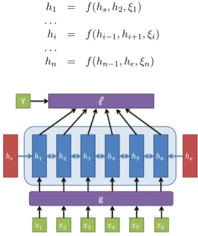
There are many potential ways to architect a neural network – in fact, this flexibility is one of deep learning’s best features – but we restrict our discussion to the structure depicted in Figure2. In this setup, we have the following variables:

data X

labels Y

parameters θ

and functions:

input layer transformation ξ=g(θ, X)

implicit hidden layer def. H=F(θ, ξ, H)

loss function L=`(θ, H, Y)

Our implicit definition function,F, is made up of local state transitions and forms a system of nonlinear equations that require solving, denoting nas the length of the input sequence andhs,heas

boundary states:

h1 = f(hs, h2, ξ1) . . .

hi = f(hi−1, hi+1, ξi)

. . .

[image:2.595.73.292.540.615.2]

hn = f(hn−1, he, ξn)

(3)

2.3 Computing the forward pass

To evaluate the network, we must solve the equa-tionH=F(H). We computed this via an

approx-imate Newton solve, where we successively refine an approximationHnofH:

Hn+1 =Hn−(I− ∇HF)−1(Hn−F(Hn))

Letkbe the dimension of a single hidden state.

(I_{− ∇}HF)is a sparse matrix, since∇HFis zero

except for k pairs of n×nblock matrices, cor-responding to the influence of the left and right neighbors of each state.

Because of this sparsity, we can apply Krylov subspace methods (Knoll and Keyes, 2004), specifically the BiCG-STAB method (Van der Vorst, 1992), since the system is non-symmetric. This has the added advantage of only relying on matrix-vector multiplies of the gradient ofF.

2.4 Gradients

In order to train the model, we perform stochastic gradient descent. We take the gradient of the loss function:

∇θL=∇θ`+∇H`∇θH

The gradient of the hidden units with respect to the parameters can found via the implicit definition:

∇θH = ∇θF+∇HF∇θH+∇ξF∇θξ

= (I − ∇HF)−1(∇θF+∇ξF∇θξ)

where the factorization follows from the noting that

(I_{− ∇}HF)∇θH=∇θF+∇ξF∇θξ.

The entire gradient is thus:

∇θL=∇H`(I− ∇HF)−1(∇θF+∇ξF∇θξ)

+_∇θ`

(1) Once again, the inverse ofI _{− ∇}HF appears, and

we can compute it via Krylov subspace methods. It is worth mentioning the technique of computing parameter updates by implicit differentiation and conjugate gradients have been applied before, in the context of energy minimization models in im-age labeling and denoising (Domke,2012).

2.5 Transition Functions

Recall the original GRU equations (Cho et al., 2014), with slight notational modifications:

final h ht= (1−zt)ˆht+zt˜ht

candidate h ˜_h_t_{= tanh(}_{W x}_t₊_U₍_r_tˆ_h_t_{) + ˜}_b₎

update weight zt=σ(Wzxt+Uzˆht+bz)

reset gate rt=σ(Wrxt+Urhˆt+br)

We make the following substitution for ˆ_h_t

(which was set toht−1 in the original GRU def-inition):

state comb. ˆ_h_t₌_sh_t

−1+ (1−s)ht+1 switch s= _spsp₊_sn

prev. switch sp =σ(Wpxt+Upht−1+bp)

next switch sn=σ(Wnxt+Unht+1+bn)

(2) This modification makes the architecture both implicit and bidirectional, sinceˆ_h_t_{is a linear}

com-bination of previous and future hidden states. The switch variablesis determined by a competition between two sigmoidal unitsspandsn,

represent-ing the contributions of the previous and next hid-den states, respectively.

2.6 Implementation Details

We implemented the implicit GRU structure us-ing Theano (Bergstra et al., 2011). The product

∇HF vfor variousv, required for the BiCG-STAB

method, was computed via theRop operator. In computing∇θL(Equation1), we noted it is more

efficient to compute∇H`(I − ∇HF)−1 first, and

thus used theLopoperator.

All experiments used a batch size of 20. To batch solve the linear equations, we simply solved a single, very large block diagonal system of equa-tions: each sequence in the batch was a single block matrix, and we input the encompassing ma-trix into our Theano BiCG solver. (In practice the block diagonal system is represented as a 3-tensor, but it is equivalent.) In this setup, each step does receive separate update directions, but one global step length. hS and he were fixed at zero, but

could be trained as parameters.

(4)

“one-step” approximation: Hidden states of a tra-ditional GRU were computed in both forward (hf

i)

and reverse (hb

i) directions, andhi was initialized

tof(hf_i₋₁, hb

i+1, ξi). If either of the two candidates

converged, we took its value and stopped comput-ing the other. We also limited both the number Newton iterations and BiCG-STAB iterations per Newton iteration to 40.

3 Experiments

3.1 Biased random walks

We developed an artificial task with bidirectional sequence-level dependencies to explore the perfor-mance of our model. Our task was to find the point at which a random walk, in the spirit of the Wiener Process (Durrett,2010), changes from a zero to nonzero mean. We trained a network to predict when the walk is no longer unbiased. We generated algorithmic data for this problem, the specifics of which are as follows: First, we chose an integer interval lengthNuniformly in the range1to40. Then, we chose a (continuous) time

t0 _∈[0, N), and a directionv_{∈ R}d. We produced the input sequencexi ∈ Rd, setting x0 = 0and iteratively computingxi+1=xi+N(0,1). After

timet, a bias term ofb_·vwas added at each time step (b·v_·(t0₋t))for the first time step greater than

t0.bis a global scalar parameter. The network was fed in these elements, and asked to predicty = 0

for timest_≤t0 andy = 1for timest > t0. For each architecture,ξwas simply the unmod-ified input vectors, zero-padded to the embedding dimension size. The output was a simple binary logistic regression. We produced 50,000 random training examples, 2500 random validation exam-ples, and 5000 random test examples. The implicit algorithm used a hidden dimension of 200, and

the b-LSTM had an embedding dimension rang-ing from100to1000. b-LSTM dimension of300

was the point where the total number of parame-ters were roughly equal.

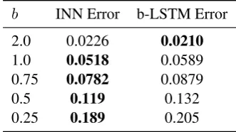
The results are shown in Table1. The b-LSTM scores reported are the maximum over sweeps from 100 to 1500 hidden dimension size. The INN outperforms the best b-LSTM in the more chal-lenging cases where the bias sizebis small.

3.2 Part-of-speech tagging

We next applied our model to a real-world prob-lem. Part-of-speech tagging fits naturally in the se-quence labeling framework, and has the advantage

b INN Error b-LSTM Error

2.0 0.0226 0.0210

1.0 0.0518 0.0589 0.75 0.0782 0.0879

0.5 0.119 0.132

[image:4.595.331.497.63.156.2]

0.25 0.189 0.205

Table 1: Biased walk classification performance.

of a standard dataset that we can use to compare our network with other techniques. To train a part-of-speech tagger, we simply let L be a softmax layer transforming each hidden unit output into a part of speech tag. Our input encodingξ, is a con-catenation of three sets of features, adapted from (Huang et al.,2015): first, word vectors for 39,000 case-insensitive vocabulary words; second, six ad-ditional ‘word vector’ components indicating the presence of the top-2000 most common prefixes and suffixes of words, for affix lengths 2 to 4; and finally, eight other binary features to indicate the presence of numbers, symbols, punctuation, and more rich case data.

We trained the Part of Speech (POS) tagger on the Penn Treebank Wall Street Journal cor-pus (Marcus et al.,1993), blocks 0-18, validated on 19-21, and tested on 22-24, per convention. Training was done using stochastic gradient de-scent, with an initial learning rate of 0.5. The learning rate was halved if validation perplexity increased. Word vectors were of dimension 320, prefix and suffix vectors were of dimension 20. Hidden unit size was equal to feature input size, so in this case, 448.

(5)

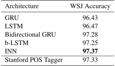
Architecture WSJ Accuracy

GRU 96.43

LSTM 96.47

Bidirectional GRU 97.28

b-LSTM 97.25

INN 97.37

Stanford POS Tagger 97.33

Table 2: Tagging performance relative to recur-rent architectures and Stanford POS Tagger.

4 Time Complexity

The implicit experiments in this paper took ap-proximately 3-5 days to run on a single Tesla K40, while the explicit experiments took approximately 1-3 hours. Running time of the solver is approx-imately nn ×nb × tb where nn is the number

of Newton iterations,nb is the number of

BiCG-STAB iterations, and tb is the time for a single

BiCG-STAB iteration. tb is proportional to the

number of non-zero entries in the matrix (Van der Vorst, 1992), in our case n(2k2 + 1).

New-ton’s method has second order convergence ( Isaac-son and Keller, 1994), and while the specific bound depends on the norm of(I− ∇HF)−1and

the norm of its derivatives, convergence is well-behaved. For nb, however, we are not aware of

a bound. For symmetric matrices, the Conjugate Gradient method is known to take O(√κ)

itera-tions (Shewchuk et al.,1994), whereκis the con-dition number of the matrix. However, our matrix is nonsymmetric, and we expect κ to vary from problem to problem. Because of this, we empiri-cally estimated the correlation between sequence length and total time to compute a batch of 20 hid-den layer states.

For the random walk experiment withb = 0.5,

we found the the average run time for a given se-quence length to be approximately0.17n1.8, with r2 = 0.994. Note that the exponent would have

been larger had we not truncated the number of BiCG-STAB iterations to 40, as the inner itera-tion frequently hit this limit for larger n. How-ever, the average number of Newton iterations did not go above 10, indicating that exiting early from the BiCG-STAB loop did not prevent the New-ton solver from converging. Run times for the other random walk experiments were very similar, indicating run time does not depend on b; How-ever, for the POS task runtime was0.29n1.3_{, with}

r2_{= 0}_.₉₁₀_.

5 Conclusion and Future Work

We have introduced a novel, implicitly defined neural network architecture based on the GRU and shown that it outperforms a b-LSTM on an artificial random walk task and slightly outper-forms both the Stanford Parser and a baseline bidi-rectional network on the Penn Treebank Part-of-Speech tagging task.

In future work, we intend to consider im-plicit variations of other architectures, such as the LSTM, as well as additional, more challeng-ing, and/or data-rich applications. We also plan to explore ways to speed up the computation of

(I_−∇HF)−1. Potential speedups include

approx-imating the hidden state values by reducing the number of Newton and/or BiCG-STAB iterations, using cached previous solutions as initial values, and modifying the gradient update strategy to keep the batch full at every Newton iteration.

6 Acknowledgements

This work would not be possible without the sup-port and funding of the Air Force Research Labo-ratory. We also acknowledge Nick Malyska, Eliz-abeth Salesky, and Jonathan Taylor at MIT Lin-coln Lab for interesting technical discussions re-lated to this work.

[image:5.595.87.272.63.170.2]

(6)

References

James Bergstra, Fr´ed´eric Bastien, Olivier Breuleux, Pascal Lamblin, Razvan Pascanu, Olivier Delalleau, Guillaume Desjardins, David Warde-Farley, Ian Goodfellow, Arnaud Bergeron, et al. 2011. Theano:

Deep learning on gpus with python. InNIPS 2011,

BigLearning Workshop, Granada, Spain.

Kyunghyun Cho, Bart van Merri¨enboer, Dzmitry Bah-danau, and Yoshua Bengio. 2014. On the properties of neural machine translation: Encoder–decoder ap-proaches. Syntax, Semantics and Structure in Statis-tical Translationpage 103.

Justin Domke. 2012. Generic methods for

optimization-based modeling. In AISTATS.

volume 22, pages 318–326.

Richard Durrett. 2010. Probability : theory and

exam-ples. Cambridge University Press, Cambridge New

York.

Jenny Rose Finkel, Trond Grenager, and Christopher Manning. 2005. Incorporating non-local informa-tion into informainforma-tion extracinforma-tion systems by gibbs

sampling. InProceedings of the 43rd Annual

Meet-ing on Association for Computational LMeet-inguistics. Association for Computational Linguistics, pages 363–370.

Alex Graves and J¨urgen Schmidhuber. 2005. Frame-wise phoneme classification with bidirectional lstm and other neural network architectures. Neural Net-works18(5):602–610.

Sepp Hochreiter and J¨urgen Schmidhuber. 1997.

Long short-term memory. Neural computation

9(8):1735–1780.

Zhiheng Huang, Wei Xu, and Kai Yu. 2015.

Bidirec-tional lstm-crf models for sequence tagging. arXiv

preprint arXiv:1508.01991.

Eugene Isaacson and Herbert Bishop Keller. 1994.

Analysis of numerical methods. Courier Corpora-tion, New York.

Dana A Knoll and David E Keyes. 2004. Jacobian-free newton–krylov methods: a survey of approaches

and applications. Journal of Computational Physics

193(2):357–397.

Christopher D Manning. 2011. Part-of-speech tag-ging from 97% to 100%: is it time for some

lin-guistics? In International Conference on

Intelli-gent Text Processing and Computational Linguistics. Springer, pages 171–189.

Mitchell P Marcus, Mary Ann Marcinkiewicz, and Beatrice Santorini. 1993. Building a large annotated

corpus of english: The penn treebank.

Computa-tional linguistics19(2):313–330.

Razvan Pascanu, Tomas Mikolov, and Yoshua Bengio. 2013. On the difficulty of training recurrent neural

networks. ICML (3)28:1310–1318.

Lawrence R Rabiner. 1989. A tutorial on hidden

markov models and selected applications in speech

recognition. Proceedings of the IEEE 77(2):257–

286.

Mike Schuster and Kuldip K Paliwal. 1997. Bidirec-tional recurrent neural networks.Signal Processing, IEEE Transactions on45(11):2673–2681.

Jonathan Richard Shewchuk et al. 1994. An introduc-tion to the conjugate gradient method without the ag-onizing pain.

Kristina Toutanova, Dan Klein, Christopher D Man-ning, and Yoram Singer. 2003. Feature-rich part-of-speech tagging with a cyclic dependency network. InProceedings of the 2003 Conference of the North American Chapter of the Association for Computa-tional Linguistics on Human Language Technology-Volume 1. Association for Computational Linguis-tics, pages 173–180.

Henk A Van der Vorst. 1992. Bi-cgstab: A fast and smoothly converging variant of bi-cg for the solution

of nonsymmetric linear systems. SIAM Journal on