Munich Personal RePEc Archive
Subjective expected utility with
imperfect perception
Pivato, Marcus and Vergopoulos, Vassili
THEMA, Université de Cergy-Pontoise, Paris School of Economics,
and University Paris 1 Panthéon-Sorbonne
8 April 2018
Online at
https://mpra.ub.uni-muenchen.de/85757/
Subjective expected utility with imperfect perception
∗
Marcus Pivato
†and Vassili Vergopoulos
‡April 8, 2018
Abstract
In many decisions under uncertainty, there are constraints on both the available information and the feasible actions. The agent can only make certain observations of the state space, and she cannot make them with perfect accuracy —she hasimperfect perception. Likewise, she can only perform acts that transform states continuously into outcomes, and perhaps satisfy other regularity conditions. To incorporate such constraints, we modify the Savage decision model by endowing the state spaceS and outcome spaceX with topological structures. We axiomatically characterize a Sub-jective Expected Utility (SEU) representation of conditional preferences, involving a continuous utility function on X (unique up to positive affine transformations), and a unique probability measure on a Boolean algebra B of regular open subsets of S. We also obtain SEU representations involving a Borel measure on the Stone space of B — a “subjective” state space encoding the agent’s imperfect perception.
Keywords: Subjective expected utility; imperfect perception; technological feasi-bility; topological space; continuous utility; regular open set; Borel measure.
JEL classification: D81.
1
Introduction
Consider the following decision problems.
(a) Doctor Ali is considering several drug treatment options for a patient. The efficacy of each drug is a continuous function of the patient’s blood chemistry, blood pressure, and other physiological variables. But many of these variables are unknown and either they are unmeasurable, or the available instruments are unreliable and imprecise.
(b) Bryant Heavy Industries (BHI) is about to build a new factory. Several different factory designs are available, using different machines and production processes. The
∗We thank Jean Baccelli, Jean-Marc Tallon and Peter Wakker for their detailed comments. We also
thank Sophie Bade, Denis Bouyssou, Alain Chateauneuf, Eric Danan, Franz Dietrich, Adam Dominiak, J¨urgen Eichberger, Spyros Galanis, Ani Guerdjikova, Simon Grant, Andrew Mackenzie, Michael Mandler, Efe Ok, Emre Ozdenoren, Michael Richter, Klaus Ritzberger and Jingyi Xue for many helpful suggestions.
future profitability of each design is a continuous function of the unpredictable market prices of several raw materials and of BHI’s final products.
(c) The Climate Emergency Panel (CEP) is considering policies to deal with climate change, including decarbonisation, mitigation, and geoengineering. The effectiveness of each policy is a continuous function of atmospheric, ecological, and economic parameters. But many parameter values are unknown, and existing measurements are unreliable and imprecise.
In all three examples, an agent must make a choice under uncertainty. The Subjective Expected Utility (SEU) model is the standard paradigm for these kinds of decisions. In the classic axiomatic foundations of Savage (1954) (and most subsequent treatments), uncertainty is described by a state space, and “acts” are functions from this state space into a space of outcomes. But the Savage theory assumes thatallpossible functions from states into outcomes are feasible, so that an agent can meaningfully form preferences over them.
This makes sense in decision problems where the state space has adiscrete topology (e.g.
bets on coins, dice, or urns; Arrow-Debreu economies). But in the three examples above, onlycontinuousfunctions are feasible, because of the underlying technological constraints. There is no drug that will transform the patient’s physiological state discontinuously into a health outcome. Likewise, there is no production process where profit is a discontinuous function of market prices. So it is ill-conceived and potentially misleading to suppose that an agent can form preferences over such infeasible acts.
Another feature of the three examples is the nature of the information available to the agent. In the standard Savage model, an agent can acquire information by observing an “event” —that is, a subset of the state space —and can form preferences conditional on this event. In the Savage model,anysubset of the state space is a potentially observable event. But in the three examples above, agents can only acquire information using unreliable and imprecise measurement devices, and many events remain unobservable.
For example, Dr. Ali might have instruments to measure the patient’s high-density lipoprotein cholesterol (HDLC) level, in milligrams per decilitre (mg/dL). Suppose her instrument can only measure concentration to the nearest mg/dL. If the instrument reports the cholesterol level as “8 mg/dL”, this means that the measured value is somewhere between 7.5 and 8.5 mg/dL. Furthermore, the machine is susceptible to a random error of 0.3 mg/dL, so Dr. Ali can only be sure that the true level is between 7.2 and 8.8 mg/dL. If she carefully repeats the measurement several times, she can reduce this error down to 0.05 mg/dL, in which case she will know that the true value is between 7.45 and 8.55 mg/dL.
Dr. Ali can also measure the patient’s low-density lipoprotein cholesterol (LDLC) level. Again, her instrument is imperfect, so it can only report an integer value, and is susceptible to error; a measurement of “11 mg/dL” means the measured value is between 10.5 and 11.5 mg/dL, which means that the true value is between 10.2 and 11.8 mg/dL. Unfortunately, to prescribe the correct medecine, she needs to know whether the totalcholesterol level —the sum of HDLC and LDLC levels —is below 20 mg/dL, and she has no instrument which can directly measure this. According to her measurements, the ordered pair (HDLC,LDLC) is confined to the box [7.45,8.55]× [10.2,11.8]. But the line described by the equation “HDLC + LDLC = 20 mg/dL” cuts through this box.
process that requires 0.1 kg of tellurium (Te) and 1 kg of ferro tungsten (FeW) per unit of output, and which will only be profitable if the combined cost of the two materials is below $70 per unit. After considerable market research (e.g. geological surveys of tellurium deposits in Kyrgyzstan), BHI believes the world price of Te will remain between $200/kg and $300/kg for the foreseeable future, while the price of FeW will be between $20/kg and $60/kg. Thus, the price vector (Te,FeW) must be in the box [200,300]×[20,60]. But the line described by the equation “0.1 Te + FeW = $70” cuts diagonally through this box.
Furthermore, some events are simply impossible to observe. For example, it might be diagnostically useful for Dr. Ali to measure the patient’s triglyceride levels, but perhaps she has no device which can do this. Likewise, the effects of different climate policies may depend partly on the structure of the methane clathrate deposits at the bottom of the Barents Sea. But it may be impossible to make any precise measurements of these deposits. So the CEP cannot condition its plans on such measurements.
One couldapply the Savage approach directly to these kinds of decision problems. But this would require the agent to form preferences over infeasible acts and to condition these preferences on unobservable events. This undermines the plausibility of the preference rela-tion, the axioms, and the resulting SEU representation —whether interpreted normatively or descriptively. For these reasons, imperfect perception and technological constraints re-quire a substantial departure from the Savage framework; this is the topic of this paper. First, we introduce a new model of imperfect perception; then, we use this model to analyse decisions under uncertainty with imperfect perception and technological constraints. We do this by enriching Savage’s state space and outcome space with topological structure.
Our model of imperfect perception has three aspects. First, we assume that the agent is only able to acquire information about the state by observing it through afinite partitionof the state space. For example, Dr. Ali is only able to measure the patient’s HDLC levels to the nearest mg/dL. It might be diagnostically useful to measure it to the nearestmicrogram per decilitre, but her instruments cannot do this. Second, only some finite partitions are
observable. For example, Dr. Ali is only able to measure certain physiological variables;
she has no way to directly measure total cholesterol or trigliceride levels. Likewise, BHI cannot directly estimate the price of the Te-FeW mixture, and the CEP cannot precisely measure the methane clathrate deposits. Finally, even for those measurements the agent
canmake, there may be a small amount of random error. The agent might be able to make
this error arbitrarily small, but she cannot reduce it to zero. So Dr. Ali can only really determine that HDLC levels are between 7.5−ǫ and 8.5 +ǫmg/dL, for some small ǫ.
To capture these three aspects, we suppose that the agent’s information about the
state arrives through a regular partition of the state space S. For example, there might
be an open, continuous function φ from S to some closed interval [a, b] of real numbers
(representing some numerical “measurement”, e.g. the HDLC level in mg/dL), along with a finite set of threshold values a =h0 < h1 < · · ·< hN = z such that the agent can only
observe events of the form “hn−1−ǫ < φ(s)< hn+ǫ” (for somen∈[1. . . N]), wheresis the
true state of the world and ǫ >0 is some measurement error. If she can make ǫ arbitrarily small, the agent can, in the limit, observe events of the form “hn−1 ≤φ(s)≤hn”. In other
words, she can observe the events φ−1[h
subsets of S, which overlap on their boundaries. For technical reasons, it is simpler (and for our purposes, equivalent) to represent these sets by theirinteriors, which are the events
R1, . . . ,RN, where Rn := φ−1(hn−1, hn) (because φ is continuous and open). These are
regular subsets of S, and their union R1 ⊔ · · · ⊔ RN is dense in S —we call this a regular
partition of S. This is the basic unit of information available to the agent in our model.
Furthermore, only certainregular partitions might be available —for example, because
only certain real-valued functions φ can be used in the above construction, because only certain “measurements” are technologically feasible. The collection of all feasible regular partitions generates a Boolean algebra B. This is the algebra of all events which are ob-servable, either directly or indirectly, by the agent. Any conditional preferences she forms
must be conditional on events in B. Meanwhile, our model represents technological
con-straints on the feasible actions by defining them as continuous functions from the state
space onto the outcome space. The domain A of feasible acts need not contain all
con-tinuous functions; thus, our framework can incorporate further technological restrictions. The agent’s conditional preferences rank acts inA conditional upon events inB.
Despite these limitations, our main results provide axiomatic characterizations of SEU representations for conditional preferences. In these representations, utility is acontinuous function; thus, similar outcomes yield similar utility levels. This makes our representations particularly relevant to applications in economics and finance, which usually take continuity for granted (Gollier, 2001). Moreover, beliefs are described by what we call a credence, a
structure like a finitely additive probability measure on the Boolean algebra B (Theorem
1). Finally, under an additional assumption on B, beliefs can also be represented by a
classical Borel probability measure on the Stone space of B —a “subjective” state space
extending the initial state space (Theorem 2).
Technological constraints introduce some obstacles into the axiomatization of SEU. For
example, Savage’s axioms (e.g. the Sure Thing Principle) and his construction of
condi-tional preferences depend on the ability to splice any two acts on any binary partition of the state space. Furthermore, Savage obtains the subjective probability measure and utility function by restricting preferences to two-valued acts and finitely-valued acts respectively. But both spliced acts and finitely-valued acts are typically discontinuous, and hence inad-missible in our framework. Furthermore, Savage’s axiom P6 (Small event continuity) relies on a rich collection of classical partitions of the state space. But in our model of imperfect perception, only certain regular partitions of the state space are available.
The rest of this paper is organized as follows: Section 2 presents our model of imperfect perception. Section 3 introduces the notation and terminology of our model of decisions under uncertainty. Section 4 introduces the six axioms used in our results. Section 5
presents the SEU representation, in terms of a credence on a Boolean subalgebra B of
regular sets, while Section 6 presents the Stonean SEU representation, which relies on
a Borel probability measure on the Stone space of B. Section 7 contains variants and
2
Imperfect perception
LetS be a topological space, which we interpret as the set of possible states of nature. An open subsetR ⊆ S isregularif R is the interior of its own closure. For example, any open interval is a regular subset of R. The union of any two non-touching open intervals is also
regular. However, the union (0,1)⊔(1,2) isnot regular, because the interior of its closure is the interval (0,2). The interior of any closed set is regular.
The intersection of two regular subsets is another regular subset. Given any two regular subsets D,E ⊆ S, we define their join to be D ∨ E := int[clos(D ∪ E)] (the interior of the
closure of D ∪ E). This is the smallest regular set containing both D and E. Meanwhile,
given a regular subsetD, we define¬D to be the interior ofS \ D—another regular subset. The set R(S) of all regular subsets ofS forms a Boolean algebra under the operations ∨,
∩, and¬(Fremlin, 2004, Theorem 314P). For example, we noted that (0,1)⊔(1,2) is not a regular subset ofR. But (0,1)∨(1,2) = (0,2) is indeed regular. Likewise, the set-theoretic
complement of (0,1) is not regular, but its interior, ¬(0,1) = (−∞,0)∪(1,∞), is.1 A regular partition of S is a collection R1, . . . ,RN of disjoint regular subsets such that
R1∨ · · · ∨ RN =S —equivalently, such that R1⊔ · · · ⊔ RN is dense inS. As we already
hinted in the introduction, we will represent the agent’s imperfect perception of the state space by a collection such regular partitions —or more precisely, by the Boolean subalgebra of R(S) which is generated by them. We will illustrate this with two models.
2.1
Imperfect measurement technology
LetR:= [−∞,∞] be the extended real line, with the natural topology.2 We will represent
a “measurement” as a function φ:S−→R with two properties:3
(i) (Stability) Small changes in the state only cause small changes in the measured value.
(ii) (Sensitivity) For any states inS, any small change in the value measured atscan be achieved by some small perturbation of s.
Formally, property (i) means that φ is continuous everwhere on S. Meanwhile, property
(ii) means that φ is an open function. Thus (i) and (ii) together imply that φ is an
open, continuous, R-valued function on S. As noted in the introduction, the agent cannot
perceive the precise value of φ. Real-life instruments do not display their measurements
with infinitely many digits of precision. (Even if they did, humans could not absorb this information.) Thus, the agent’s perception of the measurement value is filtered through
some finite partition of R into intervals. Formally, we define a measurement instrument
1What we call “regular” sets are often calledregular opensets. Symmetrically, a subsetQ ⊆ S isregular closedifQ= clos[int(Q)] —or equivalently, ifQ∁ is regular open. The regular closed sets form a Boolean algebra which is dual to the regular open sets. Thus, we could have developed the entire theory of this paper using regularclosedsets instead of regularopensets.
2That is: Rhas the usual topology, while neighbourhoods of ∞and −∞ are of the form (r,∞] and
[−∞, r), respectively, for anyr∈R. So [−∞,∞] is homeomorphic to [−1,1] in the obvious way.
to be an ordered pair (φ,H), where φ : S−→R is an open, continuous function, and
H = {h0 < h1 < h2 < · · · < hN} ⊂ R is a finite set of “threshold” values, where by
convention we fix h0 :=−∞ and hN :=∞. We assume the agent is able to observe events
of the form “the measured value is between hn−1 and hn” for each n∈[1. . . N].
Formally, this corresponds to the subsetφ−1[h
n−1, hn] inS. If the agent could make one
or both of these inequalities sharp, then she could even perceive events like φ−1[h
n−1, hn)
or φ−1(h
n−1, hn). But the measurement device inevitably has some small amount of error
—call itǫ. Thus, in practice, the agent is only able to observe events of the formφ−1(h n−1−
ǫ, hn+ǫ).4 By carefully repeating the measurement many times, or by otherwise expending
resources to increase precision, the agent can make ǫ arbitrarily small, but she cannot
reduce it to zero. In the limit, she can observe the eventFn:= T
ǫ>0 φ
−1(h
n−1−ǫ, hn+ǫ).
It is easily verified that in fact Fn=φ−1[hn−1, hn], a closed subset of S.
The family {F1, . . . ,FN} covers S. But for all n ∈ [1. . . N], the sets Fn−1 and Fn
overlap on their common boundary φ−1{h
n}. So {F1, . . . ,FN}is nota partition of S. For
alln∈[1. . . N], letGn be the event that the state is notinFm for any m6=n. Formally,
Gn := S \(F1∪ F2∪ · · · Fn−1∪ Fn+1∪ · · · ∪ FN). (1)
To understand this construction, note thatGnis precisely the set of states where the agent
can be sure thathn−1 ≤φ(s)≤hn, after sufficiently precise measurements. The following
facts are easily verified: (i)G1 =φ−1[−∞, h1),GN =φ−1(hN−1,∞], andGn=φ−1(hn−1, hn)
for all n ∈ [2. . . N −1]; (ii) for all n ∈ [1. . . N], Gn = int[Fn];5 (iii) thus, Gn is a regular
subset of S; and (iv) the collection G ={G1, . . . ,GN} is a regular partition of S. We will
useG to represent the information the agent can obtain from the measurement instrument
(φ,H). When we say “The agent observesGn”, this means that the instrument has returned
a reading which tells her that the measured value is in the interval [hn−1, hn], which means
that the true value is in the interval (hn−1−ǫ, hn+ǫ) (for some arbitrarily smallǫ > 0).
Importantly, when the agent “observes” Gn, the only thing she knows for sure is that the
true state is inFn —in particular, the state may lie on theboundary ∂Gn=φ−1{hn−1, hn}.
A measurement technology is a collection Mof measurement instruments. Let BM be
the Boolean subalgebra of R(S) generated by all sets of the form φ−1(h
n, hm), for any
instrument (φ,H) ∈ M and any hn, hm ∈ H, under application of the operations ∨, ¬,
and∩. This is the Boolean algebra of all possible events in the state space which the agent can observe through any combination of measurements with her technology.
To see why it is appropriate to close the observable events under ∨ and ¬, fix n, m∈
[1. . . N] with n≤m and letGn,m be the event that the state isnotinFp for anyp6=n, m.
Formally,
Gn,m := S \(F1∪ F2∪ · · · Fn−1∪ Fn+1∪ · · · Fm−1∪ Fm+1∪. . .∪ FN).
Thus, Gn,m is the set of states where, after sufficiently precise measurements, the agent can
be sure that the true state is either inFnor inFm. It is easily verified thatGn,m =Gn∨Gm.
4Here we define−∞ −ǫ=−∞and∞+ǫ=∞.
(b) (c) (d) (a)
Figure 1: The Boolean subalgebras from Examples 2 to 5. (a) A typical element of Bprx(R2). (b) A
typical element of Bbox(R2). (c) A typical element ofBpoly(R2). (d) A typical element of Bsmth(R2).
(Note that in each case, thenegationof the shaded set is also an element of the algebra in question.)
Likewise, for anyn∈[1. . . N], letGn be the event that the state isnotinFn. Formally,
Gn :=S \ Fn. It is then easy to see that Gn =¬Gn. Hence, the regular operations ∨ and
¬ represent the appropriate logical connectives for the set of observable events.
Typically, a measurement technologyM has the formM= Φ×H, where Φ is a set of
all open, continous functions fromS intoR satisfying certain “regularity” conditions, and
where H is the set of all finite subsets H = {−∞=h0 < h1 < h2 <· · · < hN =∞}. We
define BΦ:=BΦ×H.
Example 1. Let S =R, and let Φ be the set of all open, continuous, R-valued functions
onS. Let Bas(R) be the Boolean algebra consisting of all basicsets; that is, finite disjoint
unions of the form (a1, b1)⊔(a2, b2)⊔ · · · ⊔(aN, bN), where −∞ ≤ a1 < b1 < a2 < b2 <
· · · < aN < bN ≤ ∞. Then Bas(R) is the Boolean algebra of Φ-observable events. To
see this, note that any open, continuous function φ:R−→Ris either strictly increasing or
strictly decreasing. Thus, for any h, h′ ∈ R, the preimage φ−1(h, h′) is an open interval.
Any element ofBΦ is a finite join of intersections of such intervals. ♦
Example 2. (Proximity measurements) LetS =RN . For anys∈ S, defineφs :S−→R+
by setting φs(t) := d(s, t) for all t ∈ S. Let Φprx = {φs; s ∈ S}. It is easily verified that
these functions are all open and continuous.
LetBprx(RN) be the collection of all regular subsets of RN constructed by taking joins
and/or intersections of finite collections of open balls and/or the complements of their closures. ThenBprx(RN) is a Boolean subalgebra of R(RN). A typical element is shown in
Figure 1(a). It is easily verified that Bprx(RN) =BΦprx. This algebra describes the
infor-mation available to an agent whose measurement technology allows her to check whether the true state within a specified proximity of some target state. (For example, she can check the statement, “The true state is within distance 1.6 of the point (0,0,0)”.) ♦
Example 3. (Coordinate projections and boxes) Again, let S =RN, but now let Φ box :=
{π1, π2, . . . , πN}, where πn : RN−→R is the projection onto the nth coordinate. Clearly
these projections are open and continuous.
element is shown in Figure 1(b). It is easily verified thatBbox(RN) =BΦ
box. This algebra
describes the information available to an agent whose measurement technology allows her to check whether any particular coordinateof the true state satisfies some strict inequality. (For example, she can check the statement, “The horizontal coordinate of the state is
strictly between 1.16 and 3.24.”). ♦
Example 4. (Affine measurements and polyhedra) Again, let S =RN, but now let Φpoly
be the set of all nonconstant affine functions from S to R. (A function φ : RN−→R is
affine if φ =φ0+r for some linear functionφ0 :RN−→R and some constant r ∈R.)
A subset H ⊆ RN is a hyperplane if there is a (nontrivial) linear function φ : RN−→R
such thatH:=φ−1{r}for somer∈R. A regular subsetR ⊆RN is apolyhedronif there is a
finite collectionH1,H2, . . . ,HN of hyperplanes such that∂R= (H1∩∂R)∪· · ·∪(HN∩∂R).
(Heuristically, each of the setsHn∩∂R is one of the “faces” of the polyhedron. Note that
we do not require these polyhedra to be convex, or even connected.) Let Bpoly(RN) be the
set of regular polyhedra; then Bpoly(RN) is a Boolean subalgebra of R(RN). A typical
element is shown in Figure 1(c). It is easily verified thatBpoly(RN) =BΦ
poly. This algebra
describes the information available to an agent whose measurement technology allows her to check whether the state satisfies any finite collection of strict linear inequalities.6 ♦
Example 5. (Differentiable measurements) Let S be an open subset of RN, and let
Φsmth :={φ :S−→R; φ is differentiable and dφ is everywhere nonzero}. Then Φsmth is a
collection of continuous, open functions (by the Open Mapping Theorem).
A subsetH ⊆RN is asmooth hypersurfaceif there is a differentiable functionφ:RN−→R
such thatH:=φ−1{r}for somer∈R, and such that dφ(h)6= 0 for allh∈ H. We will say
that a regular subset R ⊆ S has a piecewise smooth boundary if there is a finite collection
H1,H2, . . . ,HN of smooth hypersurfaces such that∂R = (H1∩∂R)∪ · · · ∪(HN∩∂R). Let Bsmth(RN) be the set of regular subsets ofRN with piecewise smooth boundaries. A typical
element is shown in Figure 1(d). It is easily verified thatBsmth(RN) = BΦ
smth. This algebra
describes the information available to an agent whose measurement technology allows her to check whether the state satisfies any finite collection of strict inequalities based on differentiable functions. We normally assume that the output of any scientific instrument is a differentiable function of the true state of the world; thus, Bsmth(RN) describes the
information available through such scientific instruments.7 ♦
In Examples 1 to 5, all measurements ranged over R. But ifS is acompact space, then
we must allow R-valued measurements, because there are no open continuous functions
from a compact space into R. For instance, Example 5 can be generalized to any smooth
manifoldS, by defining Φsmthto be the set of Morse functionsonS (Pivato and
Vergopou-los, 2018c, Example 4.2(b)). But if S is a compact manifold, then these functions must
range over a closed interval (which we can take to be R without loss of generality).
6This construction works if S is any topological vector space. But we must then stipulate that φ is
continuousas well as linear.
7We can also construct subalgebras ofB
2.2
Imperfect observations of a metric space
The construction in Section 2.1 is fairly general, but it does not cover all cases of inter-est. First, it does not seem possible to obtain the entire Boolean algebra R(RN) from a
measurement technology. Second, if S is a totally disconnected space (e.g. a Cantor set),
then there arenoopen continuous functions from S intoR; thus, we cannot represent any
regular subset ofS in terms of such “measurement instruments”. So we will now introduce
a second and more general model of imperfect perception. In this case, we will suppose that the state space S is a metric space.
Let ψ : S−→[1. . . N] be an arbitrary function, representing an “observation device”. For all n∈[1. . . N], let Pn :=ψ−1{n}; then{P1, . . . ,PN}be is a partition of S —that is,
P1, . . . ,PN are disjoint, andP1⊔ · · · ⊔ PN =S. As in Section 2.1, these observations are
subject to some error of size ǫ > 0, but now this error is measured in terms of the metric ofS. If the device reports the reading “n”, then the agent does not know for sure that the true state lies in Pn; she only knows that it lies in the ǫ-neighbourhoodPnǫ, defined
Pǫ
n := {s ∈ S ; d(s, p)< ǫ for some p∈ Pn}. (2)
Again, by making repeated, careful observations, the agent can makeǫ very small, but she
cannot reduce it to zero. In the limit, she can observe the set
Fn := \
ǫ>0
Pǫ
n. (3)
It is easily verified thatFn := clos(Pn).8 Once again, the collection{F1, . . . ,FN}coversS,
but it is isnota partition ofS, because these sets may overlap on the topological boundaries of the sets P1, . . . ,PN. For any n ∈ [1. . . N], we could define Gn as in formula (1). But
assertions (ii)-(iv) beneath formula (1) are not necessarily true. The reason is simple: if
P1, . . . ,PN are arbitrary subsets of S, then their boundaries may cover large regions inS.
(Indeed, if Pn is dense in S, then ∂Pn = S). Thus, the aforementioned ǫ-imprecision in
observation, even in the limit when ǫ is reduced to zero, may almost completely destroy
whatever information was carried in the original partition P.
To avoid this problem, the agent must make observations using “neat” partitions of S. A subset P ⊆ S is neat if (i) int[clos(P)] ⊆ P and (ii) P ⊆ clos[int(P)]. Inclusion (ii) means that every element of P is a cluster point of its interior. Inclusion (i) is equivalent to saying that int(P) = int[clos(P)]; in other words, the interior of P is as large as it can be, inside clos(P). In particular, int(P) is regular. It is easily verified thatP is neat if and only ifP∁ is neat. (However, the collection of neat sets does not form a Boolean algebra.) Also, if P is neat, then its boundary ∂P is nowhere dense. A partition {P1, . . . ,PN}
is neat if P1, . . . ,PN are neat. For example, if (φ,H) is a measurement technology (as
defined in Section 2.1), then for all h, h′ ∈ H, the setφ−1[h, h′
) is neat; thus, the partition
{φ−1[−∞, h
1), φ−1[h1, h2), . . . , φ−1[hn−2, hn−1), φ−1[hn−1,∞]} is neat.
8The argument of this section doesnot crucially rely on the existence of a metric onS. Assuming only
Let P = {P1, . . . ,PN} be a neat partition. For all n ∈ [1. . . N], define Fn using
formulae (2) and (3), and then defineGn via formula (1). It is now easy to verify assertions
(ii)-(iv) beneath formula (1). In particular, G := {G1, . . . ,GN} is a regular partition of
S. We will use G to represent the information the agent learns from the observation
represented by P. When we say “The agent observes Gn”, this means her device reports
“n”, which only means that thetruevalue is in the neighbourhoodPǫ
n(for some arbitrarily
small ǫ > 0). Importantly, when she “observes” Gn, the only thing she knows for sure is
that the true state is in Fn —in particular, the state may lie on the boundary ∂Gn.
We define an observation technology to be a collection O of neat partitions of S; this can be seen as a generalization of the measurement technologies introduced in Section 2.1.
Given an observation technology O, let BO be the subalgebra of R(S) generated by all
elements Gn defined using formula (1) as in the previous paragraph, under application of
∨, ∩ and ¬. This is the Boolean algebra of all possible events which the agent can learn
through any combination of observations via her technology. In particular, if we allow O
to be the set of all neat partitions of S, then BO=R(S).
There are several other models of “imperfect perception” which lead to regular parti-tions. In one of these, observations are represented by upper hemicontinuous multifunctions fromS into a finite set. In another, observations are represented byrandomneat partitions
of S (with the randomness concentrated on the boundaries). Finally, if we suppose that
meager subsets of S have “measure zero”, then we only need to define partitions “almost
everywhere”, as is typically done in classical probability theory. In this case, regular par-titions emerge as canonical representatives of these a.e. equivalence classes. However, the technical details of these alternative interpretations are beyond the scope of this paper; we refer the reader to Pivato and Vergopoulos (2018a) for details.
3
Acts and preferences
Let S and X be topological spaces. As in Section 2, elements of S represent states of
nature. Elements of X are called outcomes; they represent the possible consequences of
actions. We will assume X is connected.
Information. We will represent the agent’s imperfect perception by means of two Boolean
subalgebras B ⊆ R(S) and D ⊆ R(X), as explained in Section 2. If B ∈ B, then a B
-partitionof B is a collection{B1, . . . ,BN} (for some N ∈N) of disjoint elements ofBsuch
that B=B1∨ · · · ∨ BN. We define D-partitions similarly. We suppose that the agent can
only observe states and outcomes through B-partitions and D-partitions.
Recall that a subset Y ⊆ X is relatively compact if its closure clos(Y) is compact.
(It follows that any continuous, real-valued function on X is bounded when restricted
to Y.) For example, if X is a metric space, then Y is relatively compact if and only
if Y is a bounded subset of X. A function α : S−→X is bounded if its image α(S) is
relatively compact in X. If X is a metric space, then this agrees with the usual definition of “bounded”. But this definition makes sense even if X is nonmetrizable. LetC(S,X) be the set of all continuous functions fromS intoX, and letCb(S,X) be the set of allbounded
continuous functions from S into X. We will assume that all feasible acts lie in Cb(S,X).
An act can indirectly yield information about the state. To see this, let α:S−→X be
an act, and let s ∈ S be the state. The agent can acquire information about s by first
applyingα tos and then obtainingD-observable information about α(s). In a model with
perfect perception, we would formalize this by saying that, for any D ∈D, the agent can
check whether α(s) is inD. But we are assuming imperfect perception. So the agent can only learn whetherα(s) is in clos(D). Thus, if she is obtaining information about the state of the world via α, then she can only learn whether s is α−1[clos(D)]. As in Section 2,
we represent this observation with the regular set int (α−1[clos(D)]). Roughly speaking,
we say thatα is “comeasurable” if this observation conveys no new information about the
state, beyond the information already contained in the algebra B. Formally, a continuous
function α :S−→X is comeasurable with respect to B and D (or (B,D)-comeasurable) if int (α−1[clos(D)])∈B for all D ∈D.
Example 6. (a) If α : S−→X is any continuous function, then α is comeasurable with respect to R(S) and R(X) (because the interior of any closed set is regular).
(b) Let S = X = R, and let B = D = Bas(R) be the Boolean algebra of basic sets
from Example 1. A continuous function α : R−→R is (B,D)-comeasurable if there is a
finite sequence of points −∞ = r0 < r1 < r2 < r3 < · · · < rN = ∞ such that for each
n ∈[1. . . N], eitherφ is non-increasing on (rn−1, rn), or φ is non-decreasing on (rn−1, rn).
In particular, any polynomial is (B,D)-comeasurable, as is any decreasing or
non-increasing continuous function. Butφ(x) = sin(x) is not (B,D)-comeasurable.
(c) LetS =RN and X =RM and let B=B
poly(RN) andD=Bpoly(RM) be the algebras
of regular polyhedra, from Example 4. A function φ : RN−→RM is affine if φ = f0 +r
for some linear function f0 :RN−→RM and some constant r∈RM. We say φ is piecewise
affine if there is a partition P = {P1, . . . ,PN} of RN into regular polyhedra, and a set
φ1, . . . , φN :RN−→RM of affine functions, such thatf
↿Rn =φ n
↿Rn for alln ∈[1. . . N]. Any
continuous piecewise affine function from RN to RM is (B,D)-comeasurable.
(d) Again, let S = RN and X = RM and let B = Bsmth(RN) and D = Bsmth(RM) be
the Boolean algebras of regular sets with piecewise smooth boundaries, from Example 5. If φ : RN−→RM is any differentiable function such that the Jacobian matrix Dφ(s) is
nonsingular for all s∈RN, then φ is (B,D)-comeasurable. ♦
LetCb(S,B;X,D) denote the set of bounded, (B,D)-comeasurable and continuous
may be additional feasibility restrictions on acts, beyond boundedness, comeasurability and continuity. Thus, we introduce an exogenously given subset A ⊆ Cb(S,B;X,D); this
is the set of feasible acts. In general, A could be much smaller than Cb(S,B;X,D). For
instance, in the case whereB=R(S) andD=R(X), if feasible production plans must be infinitely differentiable, then we could define A to be the set of all bounded and infinitely
differentiable functions from S to X. However, the collection A cannot be too small; it
must be large enough to satisfy structural condition (Rch) below, and must contain all constant acts; these representsrisklessalternatives. The inclusion of such acts in Ameans that we can risklessly obtain any outcome by a feasible act.
Conditional preference structures. Savage (1954) started from a preference order on the set of unconditional acts. He then obtained conditional preferences via axiom P2 (the Sure Thing Principle). Axiom P2 assumes that, for any two feasible acts α and β, and any event B, the “spliced” act αBβ (which is equal to αonB and to β on the complement
B∁) is also feasible. But such “spliced” acts are often discontinuous, hence, inadmissible in
our framework. So instead of defining conditional preferences implicitly via P2, we must
assume they exist explicitly. But we will only assume that these preferences can rank feasible acts, and we only assume preferences conditional on observable events. Thus, in terms of its primitive behavioral data, our model is not directly comparable to the Savage
(1954) theory: while Savage assumed a single preference order on the universal domain of
acts, our approach relies on acollection of preference orders on a more restrictive domain. But compared to other conditional versions of SEU (e.g. Ghirardato, 2002), our approach requires less data, both in terms of the number of preference orders and their domain.
For any B ∈B, and any α∈ A, let α↿B denote the restriction of α to a function on B.
LetA(B) := {α↿B; α∈ A} be the set of acts conditional uponB. LetB be a preference
order onA(B). We interpretB as the conditional preferencesoverA(B) of an agent who,
after sufficiently precise measurements, learns that the true state lies in the closure of B. We will therefore refer to the system {B}B∈B as a conditional preference structure; this will be the primitive data of the model. Our goal is to axiomatically characterize an SEU representation for {B}B∈B.
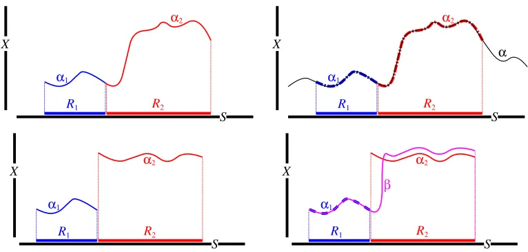
The richness condition. As already noted, the restriction to continuous acts means that we cannot rely on “spliced” acts the way that Savage did. Instead, we will require the set A of feasible acts to satisfy a “richness” condition with respect to the conditional preference structure {B}B∈B. Let B1,B2 ∈ B be disjoint regular subsets of S. For any
α1 ∈ A(B1) and α2 ∈ A(B2), say that α1 and α2 are compatible if there is some α ∈ A
with α↿B1 =α1 and α↿B2 =α2. We need A to satisfy the following condition:
(Rch) For any disjoint regular subsets B1,B2 ∈B, and any α1 ∈ A(B1) and α2 ∈ A(B2),
there is an act β2 ∈ A(B2) which is compatible with α1, such thatα2 ≈B2 β2.
In other words, the values of an act on a regular subsetB1 do not restrict the indifference
class of that act conditional upon the disjoint regular subset B2, in spite of the continuity
X
S
R1 R2
α1
α2
X
S
R1 R2
α1
α2
α
X
S
R1 R
2 α1
α2
X
S
R
1 R2
α1
α2
[image:14.612.110.493.94.277.2]β
Figure 2: Top row. α1is compatible with α2. Bottom row. The richness condition.
not very restrictive; often, every element of A(B2) is compatible with α1. The nontrivial
case of (Rch) is when B1 and B2 are “touching” –e.g. when B1 =¬B2. In this case, (Rch)
provides a weak version of Savage’s act splicing: For any B ∈B, and any α, β ∈ A, there is someγ ∈ A that is equal to α onB and indifferent toβ↿¬B conditional on ¬B. (Rch) is
also similar to solvability, a condition often used in axiomatizations of additive utility.
Aneed not containallbounded continuous functions fromS toX, as long as it satisfies
(Rch) and contains all constant acts. For example, suppose S and X are differentiable
manifolds (e.g. open subsets of Euclidean spaces RN and RM, for some N, M ≥ 1), and
let A be the set of all differentiable functions from S to C; then a conditional preference
structure on A can easily satisfy (Rch) along with our other axioms.9 Alternatively, let
S and X be metric spaces, let c ∈ (0,1], and let A be the set of all c-H¨older-continuous functions from S toX; then (Rch) is easily satisfied.10 Or, letS be a bounded interval in R, letX be a path-connected metric space, and letAbe the set of all continuous functions
from S into X having bounded variation; then again (Rch) is easily satisfied.11 But if S
and X are open subsets of Euclidean spaces, and Ais a set of analyticfunctions fromS to
X (e.g. polynomials), then a conditional preference structure onA cannotsatisfy (Rch).12
9The same is true ifAis the set ofN-times differentiable functions, for anyN ∈[2. . .∞]. 10A functionα:S−→X isc-H¨older-continuousif there is some constantK >0 such thatd[φ(s
1), φ(s2)]≤
K·d(s1, s2)
c
for alls1, s2∈ S. In the special case whenc= 1, these are calledLipschitz-continuousfunctions.
Any continuously differentiable function is Lipschitz.
11A functionα : [0, S]−→X hasbounded variation if its “total variation” sup{PN
n=1d[α(sn), α(sn−1)];
N ∈Nand 0≤s0 < s1<· · ·< sN ≤S}is finite. Heuristically, this means that αdoes not oscillate too
violently; it describes a path throughX of finite total length.
12An infinitely differentiable functionα:S−→X isanalytic if it is the limit of its own Taylor series in
4
Axioms
Throughout the paper, we assume that each order B in the conditional preference
struc-ture {B}B∈B is complete (for any α, β ∈ A(B), at least one of αB β orβ B α holds),
transitive (for any α, β, γ ∈ A(B), if α B β and β B γ, then α B γ), and nontrivial
(there exist α, β ∈ A(B) such that α ≻B β). These assumptions are more natural in our
framework than in Savage’s: they only require a transitive ordering on feasible acts, not
on all logically possible acts. To understand the implications of this distinction, consider
a case where an agent observes event B ∈ B, and must choose between two feasible acts
α and γ in A(B). Suppose that she has preferences over unfeasible acts, and there is an
unfeasible act β such that α B β and β B γ. A blind application of transitivity would
yield α B γ. But the unfeasibility of β undermines the meaningfulness of both rankings
α B β and β B γ. Why should these two rankings influence the choice between α and
γ? By restricting preferences to feasible acts, we eliminate such spurious influences.
The separability axioms. Additive separability over disjoint events is a characteristic feature of SEU theories. In a Savage framework, it is captured by P2. In Ghirardato’s (2002) axiomatization, where an agent is endowed with conditional preferences, separability is captured by the axiom of Dynamic Consistency. Dynamic Consistency also plays a central role in Hammond’s (1988) derivation of SEU maximization on decision trees; see
also Hammond (1998, §6-§7). Our next axiom captures separability through a version of
Dynamic Consistency that only applies to regular partitions of a regular event.
(Sep) For any event B ∈ B, any disjoint events D,E ∈B such that D ∨ E =B, and any
α, β ∈ A(B) with α↿D ≈D β↿D, we have αB β if and only if α↿E E β↿E.
In (Sep), the “forward implication” (from α B β to α↿E E β↿E) says that a feasible act
that was deemed optimal conditional on B will be still be optimal conditional on E. The
“backward implication” says that a more-informed decision is more reliable than a less-informed decision; thus, decisions based on inferior information should be guided by the
hypothetical decisions thatwould have been made withsuperior information. In this case,
the agent should choose α over β given inferior information (B), because she recognizes
that shewould be willing to chooseα given superior information (either D or E).
Just as the restriction to feasible acts strengthens the appeal of the ordering axiom, the restriction to events inBstrengthens the appeal of (Sep) —more specifically, its “backward
implication”. To see this, suppose the agent must choose between two feasible acts α and
β, conditional on some B ∈ B. Say that she has preferences conditional upon events D
and E, with D ∨ E = B, such that α↿D ≈D β↿D and α↿E E β↿E. A na¨ıve application of
separability would then yield α B β. But if D and E are not elements of B, then they
are unobservable events, so it is not clear that the preferences conditional on D and E are
even meaningful, much less that they should determine the choice between α and β. The
restriction toB eliminates this problem.
(i) α≻B β if and only if α↿E ≻E β↿E; and
(ii) α≈B β if and only if α↿E ≈E β↿E.
Statement (i) means that no event inB is null. Thus, any SEU representation must give
nonzero probability to all events in B. Conversely, statement (ii) says that the boundary of any event in B is null: the behaviour of α and β on that small part of B that is not covered by D ∪ E is irrelevant for decisions conditional onB. This seems to suggest that
the SEU representation must givezero probability to the boundary of any regular set. But
A is a set of continuous functions; thus, the behaviour of α and β on the open sets D and
E entirely determines their behaviour on the common boundary∂D ∩∂E. Thus, statement
(ii) does not mean that we ignorethe behaviour ofα andβ on∂D ∩∂E, as if∂D ∩∂E had zero probability; it just means that we havealreadyimplicitly accounted for this behaviour in our rankings of α↿D versus β↿D and α↿E versusβ↿E.
If D,E ∈ B are disjoint and B =D ∨ E, then Axiom (Sep) says that the B-ranking
of two actsα, β ∈ A(B) is partly determined by theD-ranking of α↿D versus β↿D and the
E-ranking of α↿E versus β↿E. The next axiom says that this dependency is continuous.
(CCP) (Continuity of conditional preferences) Let B = D ∨ E as in axiom (Sep). Let
β, α, β ∈ A(B) be three acts with β ≺B α ≺B β. Then there exist δ, δ ∈ A(D) and
ǫ, ǫ∈ A(E), with δ ≺D α↿D ≺D δ and ǫ ≺E α↿E ≺E ǫ such that, for any α′ ∈ A(B), if
δ≺D α′↿D ≺D δ and ǫ≺E α′↿E ≺E ǫ then β ≺B α′ ≺B β.
The intuition here is that a small variation inα↿D and α↿E (relative to the order topologies
onA(D) and A(E)) should not affect the B- ranking of α versus β and β.
Measurability ofex post preferences. For anyx∈ X, letκxbe the constantx-valued
act on S. Let K:= {κx; x∈ X }. We have assumed K ⊆ A, so the preference order
S,
restricted to K, induces a preference order xp onX as follows: for any x, y ∈ X,
xxp y
⇐⇒ κx
S κy
. (4)
xp describes the ex post preferences of the agent onX when there is no uncertainty. The
next axiom says that these preferences are compatible with the Boolean subalgebra D.
(M) The ex post order xp is D-measurable. That is: for all x ∈ X, the contour sets
{y∈ X; y≻xp x}and {y∈ X; y≺xpx} are elements of D.
The intuition here is straightforward. The agent is aware of her ownex postpreferences. So for any x, y ∈ X, she can discern whethery satisfies the properties “y≻xpx” or “y≺xpx”
—i.e. whetherybelongs to the open upper or lower contour set ofx. In other words, these
open contour sets must be “observable” subsets of X. But then they must belong to D.
Moreover, note that axiom (M) implies the continuity of ex post preferences with respect
Certainty equivalents. For anyB ∈Bandx∈ X, letκx
B := (κx)↿B; this is the constant
x-valued act, conditional on B. Given an act α ∈ A(B), we say x is a certainty equivalent
for α onB if κx
B ≈B α. The next axiom is a mild richness condition on X.
(CEq) For any event B ∈B, any act α∈ A(B) has a certainty equivalent on B.
Axiom (CEq) may appear somewhat implausible or technical. But it is a logical conse-quence of the following axiom of “constant measurability” which may seem more natural and has an interpretation similar to that of axiom (M).
(CM) For any event B ∈ B and any act α ∈ A(B), the sets {x ∈ X; κx
B ≻B α} and
{x∈ X; α≻B κxB} are elements of D.
If X is connected and A ⊆ Cb(S,B;X,D), then (CM) is equivalent to the conjunction of
(M) and (CEq). So we could state our results with (CM) in place of (M) and (CEq).
The statewise dominance axiom. Our next axiom imposes some consistency between the agent’s conditional preference structure and her ex post preferences. It says that the agent always prefers a statewise dominating act.
(Dom) For any B ∈B and any α, β ∈ A(B), if α(b)xp β(b) for all b ∈ B, then α B β.
Furthermore, for anyB ∈ Band any x, y ∈ X, if x≻xpy, thenκxB ≻B κyB.
Recall that, although the agent has observed the event B, the state of the world might
actually be in ∂B. (Dom) says that the values of acts on ∂B do not matter for statewise
dominance. To see why this is reasonable, recall that α andβ are continuous functions on
B, so they have unique extensions to clos(B), and these extensions preserve weak statewise
dominance. Thus, weak statewise dominance over B implies weak statewise dominance
over clos(B); that is, over all the states that remain possible given the observation of B. (Dom) appears similar to (Sep), and thus to Savage’s axiom P2. The difference is that (Sep) applies to regular partitions, while (Dom) applies to partitions into singleton sets,
which, in general, are not regular. Thus, (Dom) cannot be obtained as a special case of
(Sep). Axiom (Dom) is also related to Savage’s axioms P3 and P7. Axiom P3 requires the ranking of outcomes to be independent of the events that yield the outcomes. (Dom) entails a similar form of state independence: it implies that S can be replaced by B for
any B ∈ B, in formula (4). Thus, the ex post preference orders obtained from different
conditional preference orders must agree with one other. To see how (Dom) and P7 overlap,
consider the special case of (Dom) where one of α or β is a constant act. In fact, under
(CM) and as long as A only contains continuous and bounded acts, (Dom)implies P7.
Tradeoff consistency. To state the last axiom, we need some preliminary definitions.
Let B ∈ B, and let Q := ¬B. Consider an outcome x ∈ X and an act α ∈ A(Q).
Structural condition (Rch) yields an act (xBα)∈ A with two properties:
We will call (xBα) an (x, α)-bet for B; if B obtains, this bet is indifferent to the outcome
x, while it is indifferent to α conditional on the complement of B. Note that (xBα) is not
uniquely defined by (B1) and (B2). But if (xBα) and (xBα)′ are two acts satisfying (B1)
and (B2), then axiom (Sep) implies that (xBα)≈S (xBα)′.
Fix now four outcomes x, y, v, w ∈ X, and a regular subset B ∈B. Let Q:=¬B. We
write (x B
❀y)(v B
❀w) if there exist α, β ∈ A(Q), an (x, α)-bet (xBα)∈ A, a (y, β)-bet
(yBβ)∈ A, a (v, α)-bet (vBα)∈ Aand a (w, β)-bet (wBβ)∈ A such that (xBα)S (yBβ)
while (vBα)S (wBβ). By the remark in the previous paragraph, this implies that for any
such bets (xBα),(yBβ),(vBα),(wBβ)∈ A, we have (xBα)S (yBβ) and (vBα)S (wBβ).
If (xBα)S (yBβ), then the “gain” obtained by changing xtoy onB is at least enough
to compensate for the “loss” incurred by changing α to β on Q. In contrast, if (vBα) S
(wBβ), then the gain obtained by changing v tow on B is at most enough to compensate
for the loss incurred by changingαtoβ onQ. Together, these two observations imply that the gain obtained from changing xto yonB is at least as large as the gain from changing
v to w on B; hence the notation (x B
❀ y) (v B
❀ w). If S has an SEU representation
with utility functionu, then (x B
❀y)(v B
❀w) means thatu(y)−u(x)≥u(w)−u(v).
Conversely, we write (x B
❀ y) ≺ (v B
❀ w) if there exist γ, δ ∈ A(Q), an (x, γ)-bet (xBγ) ∈ A, a (y, δ)-bet (yBδ) ∈ A, a (v, γ)-bet (vBγ) ∈ A and a (w, δ)-bet (wBδ) ∈ A
such that (xBγ)S (yBδ) while (vBγ)≺S (wBδ). Again, this implies that (xBγ)S (yBδ)
and (vBγ) ≺S (wBδ) for any such bets (xBγ),(yBδ),(vBγ),(wBδ)∈ A. If S had an SEU
representation, then this means that u(y)−u(x)< u(w)−u(v). Here is our final axiom:
(TC) For any two regular subsets B1,B2 ∈ B, there are no x, y, v, w ∈ X such that
(x B1
❀y)(v B1
❀w) while (x B2
❀y)≺(v B2 ❀w).
In the case B1 = B2, (TC) requires “tradeoff attitudes” over outcomes to be well-defined,
independently of the acts that are used to reveal them. In the caseB1 6=B2, (TC) requires
tradeoff attitudes at different regular subsets to be consistent with each other: they must be independent of the event over which outcomes are traded. Thus, tradeoff attitudes can be evaluated independently from the choice situation used to reveal them.
Previous axiomatizations of SEU using a tradeoff consistency axiom (e.g. Wakker’s
(1988) Cardinal Coordinate Independence) did not also require a separability axiom,
be-cause it was implied by tradeoff consistency. But our axiom (Sep) is not superseded by
(TC); to the contrary, (Sep) is necessary to even state (TC). Axiom (TC) needs “bets”’
satisfying conditions (B1) and (B2). To construct these bets, we use (Rch). But the re-sulting construction is non-unique. To show that this non-uniqueness doesn’t matter in our formulation of (TC), we must invoke (Sep).
5
SEU representations
Beliefs. We will represent the probabilistic “beliefs” of the agent by a credence —a
precise, a credence onBis a function µ:B−→[0,1] such thatµ[S] = 1 and such that, for any finite collection {Bn}Nn=1 of disjoint elements of B, we have
µ " N
_
n=1
Bn #
=
N X
n=1
µ[Bn]. (5)
A credence µ behaves like an ordinary probability measure. For example, for any B ∈B
withµ[B]>0, we can define theconditional credenceµB by setting µB[R] :=µ[B ∩ R]/µ[B]
for all R ∈ B. Then µB also satisfies equation (5). We say that a credence µ has full
support if µ[B]>0 for all nonempty B ∈B.
An important difference from the usual definition of a measure is that additivity is
defined with respect to the operation ∨, rather than ordinary union. To explain this, it
helps to reformulate the additivity property of probability in logical terms, as follows:
IfB and B′ are two mutually exclusive statements, then the probability of the logical disjunction of B and B′ is the sum of their probabilities.
Now, suppose that statements B and B′ corresponds to some disjoint events B,B′ ∈ B
. As explained in Section 2.1, in our model of imperfect perception, the event corresponding to the disjunction of B and B′ is not B ⊔ B′
, but rather, B ∨ B′
. So the above principle requires that µ[B ∨ B′
] =µ[B] +µ[B′
].
Example 7. (a) Let S := (0,1), and let Bas(0,1) be the Boolean algebra of basic open subsets of (0,1), as defined in Example 1. For any B ∈ Bas(0,1), if B = (a, b) for some
a < b, then let µ[B] :=b−a. Next, if B =B1⊔ · · · ⊔ BN for some disjoint open intervals
B1, . . . ,BN, then define µ[B] := µ[B1] +· · ·+µ[BN]. Then µis a credence on Bas(0,1).
(b) More generally, let S = (0,1)N, and let λ be the Lebesgue measure on S. Let B be
the set of all regular subsets B ⊆ S such that λ[∂B] = 0. It is easily verified that B is a Boolean subalgebra ofR(S). Defineµ[B] =λ[B] for allB ∈ B; thenµis a credence onB. (Pivato and Vergopoulos, 2018c, Proposition 3.4). The same construction works for any
subalgebra of B; in particular, example (a) is a special case whenS = (0,1). ♦
Conditional expectation structures. From any credence, we can construct a
sys-tem of expectation functionals, which assign “expected values” to bounded, comeasurable
and continuous real-valued measurements and, in particular, to the utility profiles of
fea-sible acts. First, we need a bit of background. A continuous function h : S−→R is
B-comeasurable if, for any r ∈ R, we have int (h−1(−∞, r]) ∈ B and int [h−1[r,∞)] ∈B.
Let C(S,R) denote the vector space of all continuous, real-valued functions on S. Let
Cb(S,R) be the Banach space of bounded, continuous, real-valued functions, with the
uni-form norm k·k∞. Let CB(S) be the set of all B-comeasurable functions in Cb(S,R). This
set is not necessarily closed under addition. So, let GB(S) be the closed linear subspace of Cb(S,R) spanned by CB(S). (If B=R(S), then GB(S) = CB(S) = Cb(S,R).) For any
Anexpectation functionalonBis a linear functionalE:GB(B)−→Rsuch thatkEk
∞ = 1,
and such that, for any f, g ∈ GB(B), if f(b)≤g(b) for allb ∈ B, then E[f] ≤E[g]. If 1 is the constant function with value 1, then it follows that E[1] = 1.
Now letµbe a credence onB. Aconditional expectation structureforS that iscompatible with µis a collectionE :={EB}B∈B, where, for allB ∈ B, EB is an expectation functional
on GB(B), and furthermore, if µ[B]> 0, then for any B-partition {Bn}Nn=1 of B, and any
g ∈ GB(B), we require
EB[g] = 1
µ[B]
N X
n=1
µ[Bn]EBn[g↿Bn]. (6)
In particular, E = ES is an expectation functional on GB(S), and a version of equation
(6) holds for every B-partition of S. Equation (6) captures a key feature of Bayesianism: conditional expectations are additively separable over the disjoint events of aB-partition. Indeed, for any regular event B ∈ B with µ[B] > 0, the subcollection {ER}R∈B′, where B′ is the collection of sets in Bthat are contained inB, is itself a conditional expectation structure on B, compatible with the conditional credence µB.
If g ∈ GB(S) and B ∈ B, we will abuse notation and write “EB[g]” to mean EB[g↿B].
We say E is strictly monotonic if, for all B ∈ B and g ∈ CB(B), if g(b) >0 for all b ∈ B, thenEB[g]>0. For every credenceµ, there is a unique compatible conditional expectation
structure E; furthermore, ifµhas full support, then E is strictly monotonic (see Theorem 4.3 from Pivato and Vergopoulos (2018c)). For example, let S = (0,1)N, B ⊂ R(S) and
µbe as in Example 7(b). Then the uniqueµ-compatible conditional expectation structure
is defined as follows: for any B ∈ B and any g ∈ GB(B), EB[g] = RBg dλ, where λ is
the Lebesgue measure on S. (Pivato and Vergopoulos, 2018c, Example 4.1). For other
examples, see Pivato and Vergopoulos (2018c).
SEU representations. A continous functionu:X −→RisD-measurableif, for allr∈R,
the preimage sets h−1(−∞, r) and h−1(r,∞) are elements ofD. Let A ⊆ C
b(S,B;X,D),
and let{B}B∈B be aB-indexed conditional preference structure on A. Letu:X −→Rbe a continuous D-measurable “utility” function. Let µbe a credence onB. Let{EB}B∈B be
the (unique) conditional expectation structure that is compatible with µ. The pair (u, µ) is asubjective expected utility (SEU) representation for{B}B∈B if, for anyB ∈Band any
α, β ∈ A(B), we have
α B β
⇐⇒ EB[u◦α]≥EB[u◦β]. (7)
Since we suppose that the utility function uis D-measurable, and that all acts α ∈ A are (B,D)-comeasurable, it follows that all utility profiles u◦α:S−→R are B-comeasurable
(Pivato and Vergopoulos, 2018c, Proposition 5.4(a)). Thus, all utility profiles of feasible acts can be evaluated by any conditional expectation structure compatible with a credence
on B, and the SEU representation (7) is well-defined. In this SEU representation, the
utility function is continuous, but it need not be bounded, unlike Savage’s utility. This is
Theorem 1 Let S and X be topological spaces, with X connected. Let B and D be non-trivial Boolean subalgebras ofR(S)andR(X)respectively. Let Abe a collection of bounded continuous and (B,D)-comeasurable functions from S into X. Let {B}B∈B be a condi-tional preference structure on A which satisfies condition (Rch). Then, it satisfies (CEq),
(M), (Dom), (Sep), (CCP), and (TC) if and only if it has an SEU representation (7) with
full support. Finally, µ is unique, and u is unique up to positive affine transformation.
The SEU representation (7) axiomatically characterized in Theorem 1 portrays an agent facing three sorts of technological constraints. First, she only has limited information about states and outcomes —perhaps in the form of a small collection of real-valued functions representing “feasible measurements”. Even worse, due to limitations in her instruments or her own perception, she cannot even make these measurements precisely; instead of a continuum of measurement values, she can only discriminate a finite set of “measurement
intervals”, which determine regular partitions of S and X. These two informational
limi-tations mean that she can only perceive events arising from some Boolean subalgebras B
andDof regular subsets ofS andX. Finally, her actions are restricted to a collectionAof
continuous acts, which furthermore must be comeasurable relative to B and D. However,
if she defines probabilistic beliefs in the form of a “credence” on B, then she can compute the expected utility of every element ofA, conditional on any event inB, and in this way, she can define a conditional preference structure onA. Theorem 1 says that, given certain rationality axioms, every conditional preference structure arises in this way.
Sketch of proof. We will sketch the main steps in the construction of the SEU repre-sentation from the axioms. In the first step, we fix a B-partition P ={E1, . . . ,EN} of S
and use (Rch) to construct a mapping ΦP :XN−→A such that ΦP(x)↿En ≈En κ xn
En for any
n ∈ [1. . . N] and any x = (x1, . . . , xN) ∈ XN. This mapping induces a preference order
P on XN in the following way: For any x,y∈ XN,
xPy
⇐⇒ ΦP(x)S ΦP(y)
.
We then invoke (CCP), (M), (Dom) and (CEq) to show that this new preference order P
is continuous. By (TC), it also satisfies Cardinal Coordinate Independence. Since X is
connected, Theorem 6.2 from Wakker (1988) provides a continuous function uP : X −→R
and a probability vector (µP(E1), . . . , µP(EN))∈∆([1. . . N]) such that, for anyx,y∈ XN,
xP y
⇐⇒
N X
n=1
µP(En)·uP(xn)≥ N X
n=1
µP(En)·uP(yn) !
.
In the next step, we show that the functions uP can be taken to be independent ofP and
that the numbers µP(En) are independent from P, provided P contains En as a cell. This
follows from (Sep) and the uniqueness of Wakker’s theorem. Thus, we obtain a continuous
function u fromX toR, which can be shown to be D-measurable by axiom (M). We also
Finally, we show that the expected utility of any feasible act conditional on any ob-servable event is equal to the utility of any of its certainty equivalents. The argument uses (Sep) and (Dom), and relies on the boundedness and comeasurability of feasible acts. From there, since (CEq) provides certainty equivalents, the SEU representation easily follows.
6
Stonean SEU representations
The Stone Representation Theorem shows that any Boolean algebraBcan be represented
as a Boolean algebra of subsets of some set —the Stone space of B. This can be used to
obtain an alternative SEU representation where the agent’s beliefs are represented by the more familiar notion of a Borel probability measure.
Borel probability measures. Let S be a topological space. Let Bor(S) be the Borel
sigma-algebra ofS —that is, the smallest sigma-algebra containing all open sets. ABorel
probability measureonS is a (countably additive) probability measure on Bor(S). A Borel probability measureµisnormal if, for every B ∈Bor(S), we have µ[B] = sup{µ[C]; C ⊆ B
and C closed in S} and µ[B] = inf{µ[O]; B ⊆ O ⊆ S and O open in S}. Finally, it has
full support if µ(O)>0 for any open setO inS.
Stone spaces. LetBbe any Boolean algebra. Atruth valuationonBis a Boolean algebra
homomorphism v : B−→T, where T := {T, F} is the two-element Boolean algebra, with
the usual operations ∨, ∧ and ¬. If B is a set of propositions about the world, each of
which may be true or false, then v is a complete, logically consistent assignment of truth values to these propositions. Let σ(B) be the set of all truth valuations of B. For any
B ∈ B, let B∗
:={v ∈σ(B); v(B) =T}. The collection {B∗
; B ∈B} is a base of clopen
sets for a topology on σ(B), making it into a compact, totally disconnected Hausdorff
space, called the Stone space of B.13
In particular, let S be a topological state space, and let Bbe a Boolean subalgebra of
R(S) representing all events which are observable to the agent. Let S∗ := σ(B) be the
Stone space of B. Then, each truth valuation s∗ ∈ S∗ is a complete subjective description
of the world, as perceived by this agent. In turn, S∗
can be interpreted as the “subjective state space” of the agent.
Extensions of the feasible acts. Our Stonean SEU representation will use Borel prob-ability measures on the Stone space S∗ of B, and therefore needs the feasible acts to be
extended into functions on S∗. This requires additional structural assumptions.
A topological spaceS isHausdorffif any pair of points inScan be placed in two disjoint
open neighbourhoods. A Hausdorff space S is locally compact if every point in S has a
13The Boolean algebra structure of B is completely encoded in the topology of σ(B). To be precise,
the Stone Representation Theorem says that the map B 7→ B∗ is an isomorphism fromBto the Boolean