MASTER
THESIS
26-04-2018
Developing a Forecasting Model for the Power
Production of Wind Turbines
Mike M. J. Hesselink
Industrial Engineering and Management
Page | i
Page | ii
Developing a Forecasting Model for the Power Production of
Wind Turbines
Publication date
26-04-2018
Student
Mike M. J. Hesselink
Industrial Engineering and Management
Track: Production and Logistic Management
Supervisory committee:
University of Twente
Dr. R. A. M. G. Joosten
Dr. ir. L. L. M. van der Wegen
DVEP Energie
Joost Frank
Maarten Hofhuis
Maarten Vinke
University of Twente
Faculty of Behavioural, Management and Social sciences
Drienerlolaan 5
7522 NB Enschede
www.utwente.nl
DVEP Energie
Page | iii
Page | iv
Management Summary
De Vrije Energie Producent (DVEP) is an energy supplier and Balance Responsible Party (BRP) in the Dutch energy market. A BRP is responsible for buying and selling energy in advance on behalf of the customers in its portfolio. Each day DVEP is responsible for forecasting the energy production and usage of its entire portfolio for each hour of the next day. The forecast at 9:00 in the morning is used, so the forecast horizon is 15-38 hours ahead. Due to the volatile intraday market, an inaccurate day ahead forecast can be very costly. A large part of the portfolio of DVEP consists of wind power producers. Currently, DVEP buys the day ahead wind power forecast from Company X. This forecast is believed to be inaccurate, which is very costly. Therefore, the research goal is to develop a day ahead forecasting model for the power production of wind turbines of DVEP producers that is more accurate than Company X. The main research question is:
“How to develop a model that is able to translate day ahead weather forecasts
into power production forecasts for wind turbines of DVEP producers with
higher accuracy than Company X?”
Literature suggests that weather forecasts are essential for our forecast horizon. According to our literature review, we should use causal models such as regression to describe the relationship between historical weather forecasts and historical production data for each producer separately. Day ahead weather forecasts provide values for average wind speed, average wind direction and average temperature per hour. However, historical day ahead weather forecasts (hindcasts) are only available for the second half of 2017. Therefore, we describe the relationship between historical weather measurements and historical production data using regression models.
For each producer, we have data for the total production of all its wind turbines for each hour. Historical weather data are not available at the wind turbine site, so data from KNMI weather stations are used. For each weather station we have historical data of average wind speed, average wind direction and average temperature for each hour. A selection of 10 producers is included in the study based on location and total rated power. The aggregated rated power of all 10 producers is 45.65 MW. The average distance of producers to the closest KNMI weather station is 8.6 km. We use historical weather measurements and hindcasts from the KNMI stations of Vlissingen, Hupsel and Lelystad. We found statistical evidence that wind speed, wind direction and temperature forecasts are biased in Vlissingen, Hupsel and Lelystad. Therefore, we adjust the day ahead weather forecast for the bias, before we insert it into the regression models. The parameters of the regression models are estimated using historical weather measurements.
Page | v
Model Function
Log
log 𝑃 = log 𝛼 + β log 𝑣 + 𝑘 log 𝑇 + 𝜆 log cos(𝜃 − 𝛿
∗
𝑐∗ )
3rd degree polynomial
𝑃 = (𝑎0+ 𝑎1𝑣 + 𝑎2𝑣2+ 𝑎3𝑣3) ×
𝑘
𝑇× (𝜆 cos 𝜃 − 𝛿
𝑐 )
4th degree polynomial
𝑃 = (𝑎0+ 𝑎1𝑣 + 𝑎2𝑣2+ 𝑎3𝑣3+ 𝑎4𝑣4) ×
𝑘
𝑇× (𝜆 cos 𝜃 − 𝛿
𝑐 )
5th degree polynomial
𝑃 = (𝑎0+ 𝑎1𝑣 + 𝑎2𝑣2+ 𝑎3𝑣3+ 𝑎4𝑣4+ 𝑎5𝑣5) ×
𝑘
𝑇× (𝜆 cos 𝜃 − 𝛿
𝑐 ) Exponential
𝑃 = (𝑃𝑟(1 + (
𝛽 𝑣)
𝛼
)
−𝑦
) ×𝑘
𝑇× (𝜆 cos 𝜃 − 𝛿
𝑐 ) Logistic 4
𝑃 = (𝛼 (1 + 𝑚𝑒
−𝑣𝜏
1 + 𝑛𝑒−𝑣𝜏
)) ×𝑘
𝑇× (𝜆 cos 𝜃 − 𝛿
𝑐 ) Logistic 5 𝑃 = ( 𝑑 + (
𝑎 − 𝑑
(1 + (𝑣𝑓)
𝑏
)
𝑔
)) ×𝑘
𝑇× (𝜆 cos 𝜃 − 𝛿
𝑐 )
Table 1: Regression models using wind speed, temperature, and wind direction as predictors.
We select a top 3 regression models based on the accuracy using historical weather data. The 4th degree Polynomial, 5th degree Polynomial and the Logistic 4 model are the most accurate models. All three models are most accurate using wind speed, temperature and wind direction as predictors. Out of these three models, the 4th degree Polynomial model has the best day ahead forecast accuracy.
Model Standard Error of Regression (S) in kW
Root Mean Squared Error (RMSE) in kW
Mean
Absolute Error (MAE) in kW
Normalized Mean Absolute Percentage Error (NMAPE)
Company X 3,338 3,335 2,407 5.3%
4th degree Polynomial 4,166 4,162 3,092 6.8%
Table 2: Aggregated day ahead forecast error for Company X and our best model for the second half of 2017.
Page | vi
Preface
With this report my time as a student at the University of Twente comes to an end.
I want to thank DVEP for giving me the opportunity to conduct this interesting research project. During my graduation period I got to know many new colleagues. I immediately felt at home at the Supply Department of DVEP and want to thank my colleagues for the many laughs during my time there. Especially the skiing trip to Winterberg was really memorable. Special thanks go out to Joost Frank, Maarten Hofhuis and Maarten Vinke at DVEP for their supervision during this research project. Furthermore, I want to thank my supervisors at the University of Twente for their patience and guidance during this project. I am grateful for the guidance of Reinoud Joosten and the interesting conversations we had throughout the research project. I want to thank Leo van der Wegen for his critical points during the last phase of my research. This was really helpful and contributed to the end result.
I made some amazing friends during my study period, without them this period in my life would not have been so nice. Finally, I would like to thank my family for the unconditional support during my study years. They have always encouraged me and supported me in finishing my master’s thesis in these last months.
I hope you will enjoy reading this report. Hengelo, April 2018
Page | vii
Table of Contents
Management Summary
iv
Preface
vi
Table of Contents
vii
List of Figures
ix
List of Tables
xii
1.
Introduction
1
1.1 Introduction to DVEP 1
1.2 Research context 1
1.3 Problem description 3
1.4 Research objective and questions 4
1.5 Research scope 6
1.6 Report outline 6
2.
Review of Literature
7
2.1 Wind resource 7
2.2 Wind turbine design 11
2.3 Power output of wind turbines 13
2.4 Forecasting wind power production 17
2.5 Power curve modelling techniques 20
2.6 Regression models 23
2.7 Measuring forecast accuracy 26
2.8 Conclusion 28
3.
Current Situation
30
3.1 Available data 30
3.2 Producer and weather station selection 34
3.3 Weather data 35
3.4 Production data 38
3.5 Weather forecast accuracy 43
3.6 Cleaning the data 50
3.7 Conclusion 52
4.
Solution Design
54
4.1 General forecasting approach 54
4.2 Regression models 55
Page | viii
4.4 Evaluating day ahead forecast accuracy 62
4.5 Optimization algorithm 64
4.6 Conclusion 65
5.
Analysis of Results
67
5.1 Linear regression assumption testing 67
5.2 Accuracy using measured weather data 70
5.3 Top 3 models using measured weather data 74
5.4 Day ahead accuracy top 3 models 75
5.5 Day ahead forecast accuracy of Company X per producer 78
5.6 Aggregated day ahead forecast accuracy 80
5.7 Conclusion 82
6.
Conclusion and Recommendations
83
6.1 Conclusion 83
6.2 Limitations of our research 84
6.3 Recommendations 85
6.4 Suggestions for further research 86
Bibliography
87
Appendix A: KNMI weather stations in the Netherlands
90
Appendix B: Raw production data for Producers 1 and 2
91
Appendix C: Production versus wind direction
94
Appendix D: Production and wind speed versus temperature
95
Appendix E: Weather forecast error
97
Appendix F: Clean data power curves
98
Appendix G: Regression parameter values
99
Appendix H: 4
thdegree Polynomial power curves for day ahead weather forecasts
100
Appendix I: Correlation matrices
102
Appendix J: T-tests of weather forecast errors
104
Page | ix
List of Figures
Figure 1.1: Imbalance prices up to 10:00 and APX prices (€/MWh) for a random day. 2 Figure 1.2: Overview of buy and sell scenario on the day ahead auction. 2 Figure 1.3: Day ahead aggregated energy production forecast for wind turbines at 9:00. 3 Figure 1.4: Intraday aggregated energy production forecast for wind turbines at 9:00. 4 Figure 2.1: Average monthly wind speed and variation at a UK site (Lynn, 2012). 8 Figure 2.2: Typical plot of wind speed for a short period of time (Manwell et al., 2009). 9 Figure 2.3: Weibull Probability density function of wind speed using different shape parameter values
(Burton et al., 2001). 9
Figure 2.4: Atmospheric boundary layer with Prandtl layer and Ekman layer (Hau, 2013). 10 Figure 2.5: Schematic arrangement of a typical HAWT (Hau, 2013). 12 Figure 2.6: Cp – λ performance curve for a modern three-bladed turbine showing losses (Burton et al.,
2001). 14
Figure 2.7: Power curve of blade pitch control versus stall control (Hau, 2013). 15 Figure 2.8: Theoretical power curve for a standard 2 MW turbine (Lynn, 2012). 15 Figure 2.9: Air density as a function of the geographic altitude and temperature (Hau, 2013). 16 Figure 2.10: Wind speed, power and turbulence effects downstream of a building (Manwell et al.,
2009). 17
Figure 2.11: Input sources for forecasting wind power production (Giebel, 2003). 19
Figure 2.12: WTPC modelling techniques (Lydia et al., 2014). 20
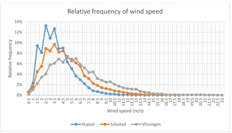
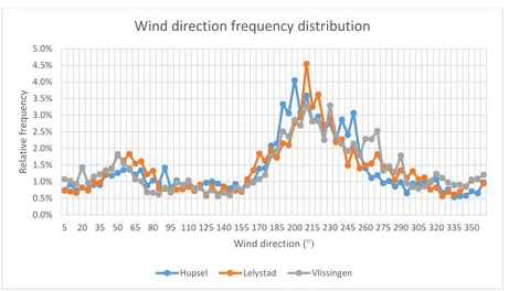
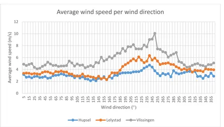
Figure 2.13: A time series divided into training- and test data (Hyndman, 2014). 28 Figure 3.1: KNMI weather stations used by DVEP located in the Netherlands (KNMI, 2000). 32 Figure 3.2: Wind speed distribution in Hupsel, Lelystad and Vlissingen in 2015-2016. 36 Figure 3.3: Wind direction distribution in Hupsel, Lelystad and Vlissingen in 2015-2016. 37 Figure 3.4: Average wind speed per wind direction in Hupsel, Lelystad and Vlissingen in 2015-2016. 38 Figure 3.5: Scatterplot of production versus wind speed in 2015-2016 for Producer 3 with 2 turbines
with 6 MW total rated power. 39
Figure 3.6: Scatterplot of production versus wind speed in 2015-2016 for Producer 1 with 2 turbines
with 1.8 MW total rated power. 40
Figure 3.7: Average production per wind direction in 2015-2016 for Producer 1 with 1.8 MW total
rated power. 41
Figure 3.8: Average production per wind direction in 2015-2016 for Producer 2 with 16 MW total
rated power. 41
Figure 3.9: Average production versus temperature in 2015-2016 for Producer 1 with 1.8 MW total
rated power. 42
Figure 3.10: Average wind speed versus temperature in 2015-2016 in Vlissingen. 43 Figure 3.11: Scatterplot of wind speed forecast errors in Vlissingen during the last 6 months of 2017.
44 Figure 3.12: Variance and average of wind speed forecast error in Vlissingen during the last 6 months
of 2017. 44
Figure 3.13: Average wind direction forecast error in Vlissingen during the last 6 months of 2017. 45 Figure 3.14: Average temperature forecast error in Vlissingen during the last 6 months of 2017. 46 Figure 3.15: Variance and average of wind speed forecast error in Hupsel during the last 6 months of
2017. 46
Page | x Figure 3.17: Variance and average wind speed forecast error in Lelystad during the last 6 months in
2017. 48
Figure 3.18: Average wind direction forecast error in Lelystad during the last 6 months in 2017. 48 Figure 3.19: Root Mean Squared Error (RMSE) for day ahead wind speed forecasts in Vlissingen,
Hupsel and Lelystad during the last 6 months in 2017. 50
Figure 3.20: Scatterplot of production versus wind speed of Producer 3 with 6 MW total rated
power. 52
Figure 4.1: Sine and cosine functions between -2π and 2π. 59
Figure 4.2: Value of cosine function for all wind directions using example of c=3 and δ=π. 60 Figure 4.3: Value of cosine function for all wind directions using example of c=10 and δ=π. 60 Figure 4.4: Parameter estimation process for Producers 1, 2, and 3. 62 Figure 4.5: Day ahead accuracy evaluation process for Producers 1-10. 63 Figure 4.6: Global versus local optima in a simplified 3D representation. 64 Figure 5.1: Scatterplot of production versus wind speed for Producer 1. 68 Figure 5.2: Scatterplot indicating heteroscedasticity for the 3rd degree Polynomial linear regression
model of Producer 1using wind speed as predictor. 69
Figure 5.3: Power curve of 5th degree Polynomial model using all 3 predictors for Producer 1 with 1.8
MW rated power using test data. 72
Figure 5.4: Power curve of 4th degree Polynomial model using all 3 predictors for Producer 2 with 16
MW rated power using test data. 73
Figure 5.5: Effect of wind direction for the best regression model for Producers 1, 2, and 3. 74 Figure 5.6: Power curve using bias adjusted hindcast data for Producer 3 with 6 MW rated power. 77 Figure 5.7: Normalized Mean Absolute Percentage Error versus wind speed for Company X for
Producers 1, 2 and 3 in the second half of 2017. 79
Figure 5.8: Normalized Mean Absolute Percentage Error versus temperature for Company X for
Producers 1, 2 and 3 in the second half of 2017. 79
Figure 5.9: Aggregated day ahead mean absolute error per hour with a total rated power of 45.65
MW in the second half of 2017. 81
Figure 5.10: Aggregated day ahead mean absolute error per month for a total rated power of 45.65
MW in the second half of 2017. 81
Figure A.1: Map of KNMI weather stations in the Netherlands. 90
Figure B.1: Scatterplot of production per wind speed in 2015-2016 for Producer 2 with 16 MW
combined rated power. 92
Figure C.1: Average production per wind direction in 2015-2016 for Producer 3 with 16 MW
combined rated power. 94
Figure D.1: Average production versus temperature in 2015-2016 for Producer 2 with 16 MW
combined rated power. 95
Figure D.2: Average wind speed versus temperature in 2015-2016 in Hupsel. 95 Figure D.3: Average production versus temperature in 2015-2016 for Producer 3 with 6 MW
combined rated power. 96
Figure D.4: Average wind speed versus temperature in 2015-2016 in Lelystad. 96 Figure E.1: Average and variance of temperature forecast error in Hupsel during the last 6 months of
2017. 97
Figure E.2: Average and variance of temperature forecast error in Lelystad during the last 6 months
of 2017. 97
Figure F.1: Scatter plot of production versus wind speed for Producer 1 with 1.8 MW total rated
Page | xi Figure F.2: Scatterplot of production versus wind speed for Producer 2 with 16 MW total rated
power. 98
Figure H.1: Power curve using day ahead weather forecast for Producer 1 with 1.8 MW rated power. 100 Figure H.2: Power curve using day ahead weather forecast for Producer 2 with 16 MW rated power.
100 Figure H.3: Power curve using day ahead weather forecast for Producer 3 with 6 MW rated power.
101
Figure I.1: Correlation matrix for Producer 1. 102
Figure I.2: Correlation matrix for Producer 2. 102
Figure I.3: Correlation matrix for Producer 3. 103
Page | xii
List of Tables
Table 1: Regression models using wind speed, temperature, and wind direction as predictors. v Table 2: Aggregated day ahead forecast error for Company X and our best model for the second half
of 2017. v
Table 2.1: Classification of wind power forecasting and its applications (Wang et al., 2011). 18 Table 2.2: Forecasting approach with different input data (Giebel, 2003). 19 Table 3.1: Example of dataset with historical weather measurements and historical production
measurements. 33
Table 3.2: Overview of available data per period of time. 34
Table 3.3: Selection of 10 producers used for analysis. 35
Table 3.4: Minimum, average and maximum production as a percentage of the rated power for
Producer 3 using raw data. 37
Table 3.5: Summary of forecast biases in Vlissingen, Hupsel and Lelystad. 49
Table 4.1: WTPC modelling techniques. 56
Table 4.2: Regression models using wind speed as predictor. 57
Table 4.3: Regression models using wind speed and temperature as predictors. 58 Table 4.4: Regression models using wind speed, temperature, and wind direction as predictors. 61 Table 4.5: Example of dataset with weather hindcasts adjusted for bias. 63 Table 5.1: Jarque-Bera test for normality of errors of linear regression models for Producer 1. 68 Table 5.2: SPSS model summary including Durbin-Watson statistic for 3rd degree Polynomial linear regression model for Producer 1 using only wind speed as predictor. 70 Table 5.3: Standard error of regression (S) for Producer 1 using different predictors. 71 Table 5.4: Standard error of regression (S) for Producer 2 using different predictors. 72 Table 5.5: Standard error of regression (S) for Producer 3 using different predictors. 73 Table 5.6: Top 3 models based on test data from Producers 1, 2 and 3. 75 Table 5.7: Bias in historical weather forecast data for the locations Vlissingen, Hupsel and Lelystad. 76 Table 5.8: Standard error of regression (S) for adjusted hindcasts of the second half of 2017. 77 Table 5.9: Root Mean Squared Error (RMSE) for Company X versus the 4th degree Polynomial model
using bias adjusted hindcast data. 78
Table 5.10: Aggregated day ahead forecast errors with a total rated power of 45.65 MW in the
second half of 2017. 80
Table B.1: Minimum, average and maximum production per wind speed for Producer 2. 91 Table B.2: Minimum, average and maximum production per wind speed for Producer 1. 93 Table G.1: Parameter values for the 4th degree Polynomial model. 99 Table G.2: Parameter values for the 5th degree Polynomial model. 99
Table G.3: Parameter values for the Logistic 4 model. 99
Page | 1
1. Introduction
In the first chapter we provide a brief description of De Vrije Energie Producent. Secondly, we describe the research context in Section 1.2. After this, we provide a problem description in Section 1.3. In Section 1.4, we formulate the research objective and research questions. Lastly, we discuss the research scope and report outline in Sections 1.5 and 1.6.
1.1
Introduction to DVEP
De Vrije Energie Producent (DVEP) from Hengelo is one of the fastest growing energy suppliers in the Netherlands. DVEP offers a wide variety of services in the energy industry, among which the supply and resupply of energy. In 2003, the organization was founded as a one-man company, after growing steadily for 14 years the company had approximately 70 employees in August 2017. In September 2017 the company was bought by UGI corporation, which is an LPG distribution company headquartered in USA with extensive operations in Europe (DVEP Energie, 2017). With approximately 13,000 employees, UGI is big international player in the LPG industry. UGI bought DVEP to have a foothold in the Dutch energy market.
DVEP trades on Dutch and German energy markets and wants expand to other countries in Europe. In addition, it also trades on energy related markets like gas. DVEP is a Balance Responsible Party (BRP), which means one of its main responsibilities is managing the usage and production of energy for energy suppliers and customers in its portfolio. DVEP is responsible for buying and selling energy on the markets on behalf of these suppliers and customers. This can involve long term deals, which usually have a fixed price per hour over a timespan of months or years, or short term (intraday) deals over a timespan of an hour or a couple of hours. Long term deals involve buying energy for a period of at least a month, long in advance for a fixed price. This is mostly done for customers with a high energy usage like municipalities or organizations, since they want to limit risk of price fluctuations. A large part of the expected energy usage is bought in advance to reduce the risk of adverse price movements. Short term deals involve eliminating energy imbalance during the day. Besides energy, DVEP is also BRP in terms of gas for some customers. However, energy is its core business.
DVEP has a wide variety of customers in its portfolio, ranging from municipalities to football stadiums. DVEP is an energy supplier and BRP for other energy suppliers. Most customers consume energy; DVEP has to estimate how much energy is consumed on an hourly basis. Besides energy users, the company has many energy producers in its portfolio as well. Most producers focus on sustainable energy like solar power, wind power, biomass, cogeneration and hydropower. Just like DVEP has to estimate the energy consumption of its portfolio, it has to estimate the energy production on an hourly basis as well.
1.2
Research context
For each day, DVEP has to hand in an estimate of the energy usage and production per hour for the following day in the form of an auction. As input for the auction, forecasts are used to estimate the hourly energy usage and production of its entire portfolio. After all BRPs have handed in their auctions, the spot market operator, APX, determines the market price for each hour of the next day based on demand and supply.
Page | 2 day, TenneT releases the predicted imbalance prices in real-time, Figure 1.1 shows the imbalance prices in €/MWh up to 10:00 for a random day.
Figure 1.1: Imbalance prices up to 10:00 and APX prices (€/MWh) for a random day.
The red line indicates the APX price, which is determined day ahead. The blue line indicates the predicted imbalance prices, these are determined by demand and supply each minute. Figure 1.1 shows that the energy imbalance market can be very volatile, with predicted prices ranging from €-150 to €140 per megawatt-hour (MWh) within one hour. The actual imbalance prices are determined per 15 minutes after the hour has passed.
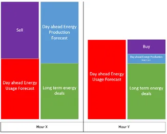
The position taken by DVEP each hour is mainly determined by the day ahead auction. Figure 1.2 illustrates a buy scenario for Hour Y and a sell scenario for Hour X at the auction.
Figure 1.2: Overview of buy and sell scenario on the day ahead auction.
Page | 3 expected production of all producers in the portfolio of DVEP. Together with the long term deals, this determines the expected amount of energy DVEP has during an hour. Depending on the energy usage and production forecasts per hour, energy is bought or sold on the auction.
The day ahead auction mainly determines the position you take for each hour of the day. During the next day, this position can be altered up until 5 minutes before the hour starts. On the intraday market, traders can buy or sell energy for upcoming hours. Some parties have excess energy based on intraday forecasts, while other parties have shortages. By selling energy to each other, they can alter their position before the hour starts. This can lower risk, because the amount that is bought/sold is not traded using imbalance prices, but the price agreed upon by both parties. As can be seen in Figure 1.1, imbalance prices can be very volatile.
According to DVEP, energy usage forecasts are quite accurate and do not form a problem. Production forecasts however, do form a problem since DVEP believes these are inaccurate. DVEP has many types of producers in its portfolio, among which solar power and wind power. Especially the wind power production forecasts are important for DVEP, since it has a lot of wind power in its portfolio.
1.3
Problem description
Currently DVEP buys a wind production forecast from a third party. We call this party ‘Company X’ out of confidentiality. The forecast from Company X shows the energy production in kilowatt-hour per hour of the day. While making the auction for the day ahead, the forecast at 9:00 is used, since the input for the auction has to be delivered before 12:00. Ideally, DVEP would like to use the forecast from 11:00. However, a time buffer for technological issues is necessary, so the 9:00 forecast is the most recent forecast that can be used. Normally, DVEP uses the exact production forecast from 9:00 of Company X in the auction. This can be seen in Figure 1.3.
Figure 1.3: Day ahead aggregated energy production forecast for wind turbines at 9:00.
The aggregated day ahead forecast at 9:00 is illustrated by the yellow line in Figure 1.3. The aggregated wind production is illustrated by the blue line, this is used in the auction that DVEP has placed before 12:00. Usually this coincides with the day ahead forecast, since DVEP uses the forecast. Therefore, the blue line is hard to see in Figure 1.3.
Page | 4 competitors. However, DVEP thinks it can be improved and wants to develop an in-house forecast model to improve forecast accuracy and lower costs. The desired output of the model is a graph that shows the expected energy production (kilowatt-hour) for each hour of the next day (see Figure 1.3). In addition to the day ahead forecast, DVEP also uses intraday forecasts so their traders have up-to-date information about the expected energy production for the upcoming hours. Since weather forecasts change during the day, the expected energy production of wind turbines changes also.
Figure 1.4: Intraday aggregated energy production forecast for wind turbines at 9:00.
Figure 1.4 shows the intraday forecast at 9:00, this forecast is based on more recent weather data. While comparing the day ahead graph in Figure 1.3 and the intraday graph in Figure 1.4, we see a difference in expected energy production (yellow line), while the auction (blue line) remains the same. To minimize the difference between the auction and the actual production, DVEP wants a more accurate day ahead forecast. Therefore, DVEP would like to develop a forecasting model that is more accurate than the current one. This model should be able to translate weather forecasts into expected wind production for DVEP wind turbines.
The core problem for this project is that the current day ahead forecast for power production of wind turbines is believed to be inaccurate. DVEP currently buys this forecast from Company X, which is costly. DVEP thinks that a forecasting model can be developed that is more accurate than Company X. DVEP is especially interested in the time horizon between 15-38 hours ahead, since this is the time horizon that is used for the day ahead auction.
1.4
Research objective and questions
The research goal is to develop a day ahead forecasting model for the power production of wind turbines of DVEP producers. This model should be more accurate than the model that is currently used. After development of the model a comparison should provide insight into which model is most accurate.
Page | 5
“How to develop a model that is able to translate day ahead weather forecasts
into power production forecasts for wind turbines of DVEP producers with
higher accuracy than Company X?”
To answer this research question, the following sub-questions are addressed during the project:
1. Which factors influence the power production of wind turbines according to the
literature?
(a) Which weather conditions influence the power production of wind turbines? (b) Which turbine characteristics influence the power production of wind turbines? (c) Which site-related factors influence the power production of wind turbines?
To determine which factors influence energy production of wind turbines, we conduct 3 literature reviews. First, we look into which weather conditions have an impact on the power production. After this, we look into wind turbine design to determine which turbine characteristics influence power performance. Lastly, we look into site-related factors.
2. What is known in literature on day ahead forecasting power production for wind
turbines?
(a) Which methods are used in literature for forecasting power production for wind turbines? (b) How can forecast accuracy be measured and the forecast model be validated?
We conduct 2 literature reviews to see which forecasting methods are used in literature for the energy production of wind turbines. We assess which forecasting method is most appropriate for the time horizon we wish to forecast. Also, we look at how to validate forecast models and how to measure forecast accuracy.
3. What is the current situation at DVEP with respect to data?
(a) Which data are available and how are these measured? (b) Which producers should be selected for model testing? (c) What are the characteristics of the available data?
Here, we look at the available data and describe how this data was measured. We make a selection of producers that are included in the project scope. We select KNMI stations throughout the Netherlands located near producers of DVEP. We analyze production and weather data and describe how we clean the data. Also, we check whether there is a bias in the weather forecasts.
4. Which forecasting approach should result in the most accurate day ahead forecast
according to the data patterns and literature review?
Page | 6
5. Which day ahead forecasting model is most accurate in production forecasts and how
accurate is this model in comparison to Company X?
In Chapter 5 we select the 3 most accurate regression models based on historical weather and production data. After this, we use historical weather forecasts for all 10 producers to see which model has the most accurate production forecast using day ahead weather forecasts as input. We do this for each producer separately, as well as for the aggregated selection of 10 producers. This enables us to compare the day ahead forecast accuracy of Company X and the models developed in this project. This leads to conclusions and recommendations in the final chapter.
1.5
Research scope
For every research project, a scope should be defined. When investigating problems, other problems may come to the surface. It is very tempting to investigate these problems as well. However, we should stick to the problem at hand. Furthermore, we are dependent on the data that are available. Therefore, we have to draw a line; we do this by defining the research scope:
The forecast horizon is 15-38 hours ahead, using weather forecasts from 9:00 in the morning as input to forecast power production for each hour of the next day.
The forecasting model focuses on accuracy in terms of production. The goal is to minimize the financial risk by being as accurate to the realized production as possible. We do not look into the financial implications of the forecasting model.
The selection of producers should cover at least 10% of the total rated power of DVEP. We assume every turbine has storm detection and ice detection.
We focus on 3 KNMI weather stations to obtain weather data.
We exclude producers with multiple sources of production (e.g. solar AND wind power), since we cannot distinguish the production of multiple sources under the same EAN (unique connection code).
We only include producers that have a contract between 01-01-2015 and 01-01-2019. We exclude producers with long term downtime between 01-01-2015 and 01-01-2019. The most important choices regarding the scope of this project are listed above. Throughout the project, the scope is further defined.
1.6
Report outline
Page | 7
2. Review of Literature
In this chapter, we conduct a literature review to obtain the information that is necessary to develop a forecasting model for the energy production of wind turbines. We answer Sub-question 1 in Sections 2.1, 2.2, and 2.3. Firstly, the wind resource is researched in Section 2.1, since this is the driving power behind the energy production of wind turbines. Secondly, in Section 2.2 we look into the types of wind turbines that are used in practice. After this, we look into the effect of turbine characteristics and site-related factors on the energy production of wind turbines in Section 2.3. Next, we answer Sub-question 2 in Section 2.4 up until Section 2.7. In Section 2.4 we review existing literature to see what forecasting methods are used in the literature. In Section 2.5, we discuss wind turbine power curve modeling techniques that are most promising. Afterwards, in Section 2.6 we show how these models can be expanded with the help of regression analysis. Lastly, in Section 2.7 we discuss how forecasting performance can be measured.
2.1
Wind resource
The winds of the world are unpredictable, intermittent, fickle in speed and direction, and are occasionally extremely strong. This poses a challenge to predict the effectivity of wind energy systems. To do so, we need to understand the wind’s behavior.
2.1.1 Wind speed variability during different timescales
The wind speed variability can have a big impact on energy production of a wind energy application. When considering variations in wind speed in time, conventional practices use four time categories (Lynn, 2012; Manwell, McGowan & Rogers, 2009):
Inter-annual. Annual.
Diurnal (time of day). Short-term.
We briefly discuss each category and its implications for wind turbines.
Inter-annual
The wind resource at a particular site differs from year to year. For example, a coastal site in the Western Europe may experience a series of strong ‘autumn gales’ one year, but not during the next (Lynn, 2012). So a single year’s wind speed measurement, although widely used to assess a site’s potential, may not always give an accurate picture. Inter-annual variations of up to 5% in average wind speed are pretty common. These variations in wind speed lead to even bigger variations in power output, as we demonstrate later on. The ability to estimate the inter-annual variability at a site is almost as important as estimating the long-term mean wind at the site. Manwell et al. (2009) state that it takes meteorologists approximately 30 years of data to determine long-term values of weather or climate, and that it takes at least five years to arrive at reliable average annual wind speed at a given location. Lynn (2012) adds that climate change can have an influence in the future as well. Who can tell what will happen to the world’s wind patterns over the coming decades?
Annual
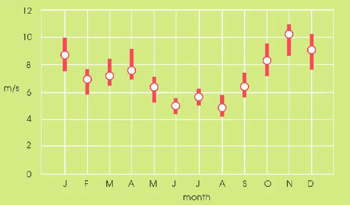
Page | 8 that the autumn and winter months tend to be most windy, summer months are the calmest. These annual variations are important when it comes to assessing wind energy production in relation to seasonal energy demand.
Figure 2.1: Average monthly wind speed and variation at a UK site (Lynn, 2012).
Diurnal (time of day)
In temperate latitudes, large wind variations can occur on a diurnal or daily time scale. This type of wind speed variation is due to differential heating of the earth’s surface during the daily radiation cycle (Manwell et al., 2009). A typical diurnal variation is an increase in wind speed during the day with lowest wind speeds during the hours between midnight and sunrise (Lynn, 2012). Daily variations in solar radiation are responsible for diurnal wind variations in temperate latitudes over flat land areas. According to Manwell et al. (2009), the largest diurnal changes occur in spring and summer, and the smallest in winter. Diurnal variation may also vary with location and altitude. At mountainous areas the diurnal variation may be very different than at flat areas. This variation can be explained by the mixing or transfer of momentum from the upper air to the lower air (Manwell et al., 2009).
Short-term
Page | 9
Figure 2.2: Typical plot of wind speed for a short period of time (Manwell et al., 2009).
When considering wind energy applications for a given location, all these time categories have to be taken into account. From long-term wind speed prediction to maximum load calculations due to gusts or turbulence, a wide variety of implications of wind speed variations need to be considered over time. For wind energy applications, knowledge of wind behavior is of particular importance to successfully utilize the kinetic wind energy. While short-term behavior of wind is of significance with regard to the structural strength and control function of a wind turbine, the long-term characteristics of the wind have relevance with regard to the energy yield (Hau, 2013). The long-term characteristics of the wind can only be determined by using statistical surveys over many years.
2.1.2 Wind speed probability distribution
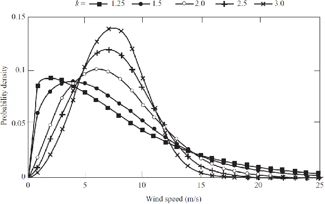
While year-to-year variation in annual mean wind speeds is hard to predict, wind speed variations during the year can be well characterized in terms of a probability distribution. In the literature it is widely found that the Weibull distribution gives a good representation of the variation in hourly mean wind speed over a year at many typical sites (Burton et al., 2001).
Page | 10 The shape parameter k determines the shape of the distribution. A special case of the Weibull distribution is the Rayleigh distribution with k=2, this is a fairly typical value for many locations (Burton et al., 2001). On real sites the shape parameter k varies from about 1.5 to 2.5. A value of 1.5 is typical for offshore sites, over land the factor reaches values up to 2.5 or somewhat above (Hau, 2013). Offshore locations typically have a longer tail, because there is less surface friction offshore. The Weibull distribution can be used to estimate annual production, the Danish manufacturer Vestas uses a shape parameter of k=2 to estimate annual production of its turbines (Vestas, 2017). For short term production estimates, the Weibull distribution is not very useful.
2.1.3 Wind speed at different altitudes
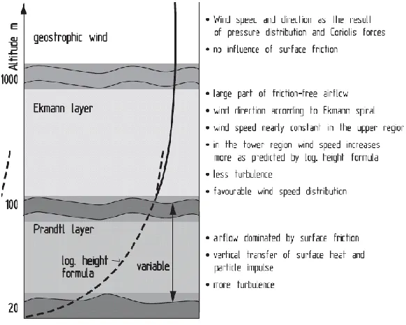
[image:23.595.76.367.369.602.2]One of the most important factors with respect to the utilization of wind energy is the increase in wind speed with altitude. The moving air masses have less friction against the earth’s surface as the altitude increases. The range up to where the wind is undisturbed is between 600 and 2000 m above ground, depending on the time of day and atmospheric conditions (Hau, 2013). This is called the atmospheric boundary layer. The area of the boundary layer closest to the ground is called the Prandtl layer, where flow conditions are dominated by the friction with the earth’s surface. In meteorology the area above the Prandtl layer is called the Ekmann layer. The influence of friction is less dominant in this layer, while wind direction is influenced by Coriolis forces due to the earth’s spin. Above the Ekmann layer, geostrophic winds flourish since there is no surface friction, and there are large influences by Coriolis forces.
Figure 2.4: Atmospheric boundary layer with Prandtl layer and Ekman layer (Hau, 2013).
The height of Prandtl layer varies with the meteorological conditions. During the night, it is only 20 to 50 m thick, whereas during the day it is between 50 and 150 m thick. A rotor hub height of 60 m is in the Prandtl layer for approximately 30% of the annual hours whereas a hub height of 100 m this is only about 7%. Therefore, the wind conditions of large turbines are extensively influenced by the characteristics of the Ekman layer (Hau, 2013).
2.1.4 Turbulence and gusts
Page | 11 with the earth’s surface and thermal effects (Burton et al., 2001). Friction with the earth’s surface can be thought of as flow disturbances caused by hills and mountains or man-made structures. Thermal effects cause air masses to move vertically due to differences in temperature and density of the air. These two effects are often interconnected. Turbulence is a complex process, in order to describe it, it is necessary to take into account the temperature, pressure, density and humidity as well as the motion of the air itself in three dimensions (Burton et al., 2001).
Wind gusts are big, short-term fluctuations in wind speed. Whereas the long-term fluctuations in wind speed are significant to the power output and energy yield of a wind turbine, the loads are marked by short-term fluctuations in wind speed (Hau, 2013). The extreme wind speeds must be taken into consideration for the fatigue strength and loads, although they may occur rarely. Wind gusts and turbulence are especially interesting for fatigue and maximum load calculations, not for power output and energy yield because of their short-term nature (Hau, 2013).
2.2
Wind turbine design
Mankind has been trying to use the wind to its advantage for a long time. The oldest windmill in recorded history is the so-called Persian windmill. It was first described around 900 AD and is a drag-driven windmill with a vertical axis of rotation (Schaffarczyk, 2014). Drag-drag-driven means the windmill generates its power by using drag force, which has the same direction as the wind. Later, in 1279 the Dutch windmill appeared which represented a milestone in technological development. The axis of rotation changed from vertical to horizontal. From an aerodynamic point of view, the Dutch concept began a movement toward lift-driven wind turbines instead of drag-driven (Schaffarczyk, 2014). Lift force refers to forces perpendicular to the wind direction. Today, a wide variety of wind turbines are used. Wind turbines can either rotate about a horizontal or vertical axis, therefore wind turbines are classified as Horizontal Axis Wind Turbines (HAWTs) or Vertical Axis Wind Turbines (VAWTs). HAWTs are the dominant design principle in wind energy technology today, since this design has a higher power output (Hau, 2013). Therefore, we take a closer look at HAWTs.
2.2.1 Horizontal axis wind turbine
Within the HAWT classification, there are a lot of variations. These variations include the number of blades, arrangement of rotor, variable/constant speed, blade pitch control and yawing options. According to Schaffarczyk (2014), standard HAWTs have the following properties:
Horizontal axis of rotation. Three bladed.
Driving forces mainly from lift.
Upwind arrangement of rotor; tower downwind. Variable speed/Tip-speed ratio (TSR) control. Blade pitch control after rated power is reached.
Page | 12
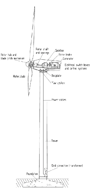
Figure 2.5: Schematic arrangement of a typical HAWT (Hau, 2013).
Most turbines have a hub height between 40 and 120 m, in extreme cases the height can go up to 180 m. Rotor blades range in length from 20 to 80 m and most turbines have 3 rotor blades. Turbines are built with a rated power of up to 8 MW today. Offshore wind turbines are usually larger than onshore ones; this typically leads to a higher rated power. Today’s onshore turbines range up to 120 m normally and rarely exceed 3 MW.
If a turbine wants to capture the full power of the wind, it has to be oriented to the wind direction correctly. Wind direction is constantly measured and the yaw system makes sure the horizontal axis of rotation is perpendicular to the wind direction. There are three different yawing methods (Hau, 2013):
Yawing by aerodynamic means (wind vanes or fan-tail wheels). Active yawing with the help of a motorized yaw drive.
Free yawing of rotors located downwind.
Page | 13 the blade and the wind speed is kept at a constant, optimal rate. This is done to achieve maximum efficiency.
The last property which we discuss is power control, in case of strong winds it is necessary to waste part of the excess energy to avoid damaging the wind turbine in high wind speeds. All wind turbines are therefore designed with some sort of power control. There are two different ways of doing this safely on modern wind turbines:
Blade pitch control. Stall control.
The most effective way of adjusting the aerodynamic angle of attack, and thus the input power, is by mechanically changing the rotor blade pitch angle (Hau, 2013). The rotor blade is turned about its longitudinal axis with the aid of actively controlled actuators with this method. This is not only done for safety measures, but also to maintain maximum output after rated power is reached.
When a turbine does not have blade pitch control, rotor blades have a fixed angle which is called stall control. Stall controlled wind turbines have blade designs that create turbulence on the side of the blade not facing the wind when the wind speed increases. As the actual wind speed increases, at some point the rotor blade starts to stall, which prevents it from reaching dangerously high speeds.
2.3
Power output of wind turbines
A wind turbine has to capture as much of the wind’s power as possible and convert it efficiently into electricity. This is done by converting kinetic energy of the wind into electrical energy. The performance of a wind turbine depends crucially on the conditions at a particular site including the wind’s average speed and variability (Lynn, 2012). To see what factors influence the power output of wind turbines, (Lynn, 2012) starts by considering a well-known equation of fluid mechanics:
𝑃 =1
2𝜌𝐴𝑣
3 (2.1)
where:
P = power in W
𝜌 = air density in kg/m3
A = area of the intercepted airstream in m2 (swept area of rotor blades) v = wind velocity in m/s
Equation 2.1 is used to calculate the available kinetic wind power. We see that the available wind power increases with the air density, the area of the intercepted airstream and the wind velocity. Especially the wind velocity has a big impact due to its cubic relationship with power. To illustrate its impact, a doubling in wind velocity leads to an eight times higher available wind power. Air density and the swept area of the rotor blades have an influence as well.
In Equation 2.1, the available wind power can be calculated. However, the power that is extracted by wind turbines is smaller. There are fundamental limitations to rotor efficiency that prevent wind turbines from converting 100% of the available wind power. Therefore, Burton et al. (2001) added a power coefficient to the equation, resulting in Equation 2.2:
𝑃 =1
2𝜌𝐶𝑝𝐴𝑣
3 (2.2)
Page | 14
𝐶𝑝 = power coefficient (fraction of the available wind power that may be converted by the turbine into mechanical work)
The power coefficient has a theoretical maximum value of 59.3% (Betz limit) due to the principles of conservation of mass and momentum of the air stream, though in practice lower peak values are reached (Burton et al., 2001). Incremental improvement in the power coefficient are constantly sought by detailed design changes in wind turbines. However, these changes only lead to a modest increase in power output. Major increases in power output can only be achieved by increasing the swept area of the rotor or by locating the wind turbines on sites with higher wind speeds (Burton et al., 2001).
2.3.1 Turbine characteristics and power output
A cause of reduced output is rotor yawing with the wind direction. Yawing is the process of aligning the rotor with the wind direction. This is done to use the wind to its highest potential. Even with sensitive yawing a certain loss is unavoidable. Various investigations have shown a loss of about 2 to 3% in energy yield of the turbine with a correctly operating yawing mechanism (Hau, 2013). Losses increase when there are frequent wind direction changes on site.
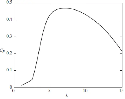
[image:27.595.75.342.363.574.2]Another cause of reduced output can be explained with the 𝐶𝑝– λ performance curve. Here, 𝐶𝑝 is the power coefficient and λ, the tip-speed ratio (TSR). The TSR is the ratio between the speed of the tip of the rotor blade and the wind speed.
Figure 2.6: Cp – λ performance curve for a modern three-bladed turbine showing losses (Burton et al., 2001).
The first thing to note is that the maximum value of 𝐶𝑝 is only 0.47, which is smaller than the Betz limit, achieved at a TSR of 7 (Burton et al., 2001). To have maximum efficiency, it is crucial that the TSR is kept at this constant rate. The fact that this value is considerable smaller than the Betz limit is due to stall, tip and drag losses among other losses.
Page | 15 An option that also affects the power output is blade pitch control. A change in angle of attack can have a big impact on the power output. Blade pitch control is also used to regulate the TSR, thus is connected with TSR control. Active pitch control is necessary to maintain a constant, optimal TSR after rated wind speed is reached (Burton et al., 2001).
Figure 2.7: Power curve of blade pitch control versus stall control (Hau, 2013).
The pitch angle should continuously be adjusted after rated power is reached to maintain the highest efficiency. This is where blade pitch control distinguishes itself from stall control. After rated power is reached blade pitch control is able to maintain optimal TSR so rated power is achieved at a wider wind range than using stall control. Figure 2.7 illustrates that stall controlled turbines are less efficient at high wind speeds.
Obviously, wind speed affects the power output of the turbine. However, wind can reach tremendous speeds, leading to dangerous situations. To prevent turbine damage, the blades can be feathered and the turbine is turned off, this happens when cut-out speed is reached. This means only a certain range in the wind speed domain can be utilized (Lynn, 2012).
Figure 2.8: Theoretical power curve for a standard 2 MW turbine (Lynn, 2012).
Page | 16 where it ideally will remain until the blades are feathered, and the turbine is shut off. Cut-in and cut-out speeds can vary depending on design type and environmental factors (Lynn, 2012). The newest turbine designs from the German manufacturer Enercon have cut-out speeds between 28-34 m/s (Enercon, 2015). However, older turbines have lower cut-out speeds.
2.3.2 Site-related influences on power output
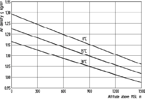
[image:29.595.75.382.212.423.2]The density of the air has an influence on power output and varies with both elevation and temperature. Cold air at sea level is considerably denser than warm air at high upland sites (Hau, 2013). This is illustrated in figure 2.9:
Figure 2.9: Air density as a function of the geographic altitude and temperature (Hau, 2013).
Air density decreases when temperatures increases from 0 °C. The density is largest at mean sea level (MSL), the decrease in air density is already noticeable at a few hundred meters, as well as the change in the temperature range between summer and winter, so that its influence on turbine performance cannot be neglected (Hau, 2013). This is supported by Lynn (2012), who states that a turbine produces more power during winter than midsummer, in winds of the same speed. Large manufacturers such as Enercon and Vestas assume a standard air density of 1.225 kg/m3 in their power curves (Enercon, 2015; Vestas, 2017).
Page | 17
Figure 2.10: Wind speed, power and turbulence effects downstream of a building (Manwell et al., 2009).
In Figure 2.10 the change in available power and turbulence is illustrated in the wake of a sloped-roof building. At a distance of 5 times the height of the building (5 hs), the wind power is decreased by 43% mainly due to an increase in turbulence and a decrease in wind speed. At larger distances the turbulence reduces and wind speeds increase again which results in a smaller loss in wind power (Manwell et al., 2009). Besides buildings and other manmade objects, wooded inland regions and mountainous areas have an impact on the annual energy yield as well (Hau, 2013). It is difficult to estimate flow conditions in complex terrain in detail. The flow field is affected by topographic shapes such as slopes or depressions. Depending on wind direction, wooded inland areas cause variable vertical wind shears (Hau, 2013). Seasonal changes need to be accounted for also, during summer the trees have a larger collection of leaves in comparison to the winter, which affects wind flow differently. Each location has its own specific air flow conditions, which have to be examined carefully when estimating annual energy yield. However, from the point of view of the practical operation of the wind turbine, the influence of turbulence on the energy yield is, as a rule, not severe (Hau, 2013).
Apart from the turbulence of the wind, other weather-related factors can influence the power output of wind turbines also. Primarily, icing of the rotor blades at temperatures below zero can alter the aerodynamic profile of the blades significantly (Hau, 2013). However, due to safety reasons the turbine has to be turned off so there is no sense in taking its influence on the power curve into consideration. The influence of snowfall or long-lasting rain can have a more practical significance. According to Hau (2013), recent studies have shown that the surface roughness of the rotor blades changes due to the rain, which can result in power losses.
Another factor that influences the surface roughness of the rotor blades is soiling. After a certain operating period, rotor blades exhibit soiling phenomena (Hau, 2013). The dirt on the surface of the blades is produced after long periods of dryness and high temperatures in summer. During this time there are more dust and insects in the air, which can stick to the blades. Soiling is not only dependent on the weather, but also on the site. Extreme conditions are observed in desert-like conditions. A prolonged operation with badly soiled rotor blades leads to a great loss in energy yield (Hau, 2013).
2.4
Forecasting wind power production
Page | 18 used for these approaches. We focus on day ahead wind power forecasting, since that is the
forecasting horizon that we use in this research.
2.4.1 Forecasting approaches for wind power production
When considering forecasting methods for power production of wind turbines, a classification of forecasting horizon needs to be made. Forecasting serves different purposes for different time-scales, for 8 hours-ahead the main purpose is real-time grid operations, while multiple-days-ahead one of the main purposes is maintenance planning (Wang et al., 2011). Table 2.1 shows the classification of wind power forecasting and its applications:
Time-scale Forecast horizon Applications
Immediate-short-term 8 hours-ahead - Real-time grid
operations
- Regulation actions
Short-term 48 hours-ahead - Economic load dispatch
planning
- Load reasonable decisions
- Operational security in spot market
Long-term Multiple-days-ahead - Maintenance planning
- Operation management - Optimal operating cost
Table 2.1: Classification of wind power forecasting and its applications (Wang et al., 2011).
In this research, we use wind power forecasting for operational security in the spot market. Besides classification based on the prediction horizon, wind power forecasts can also be classified based on their methodology. Here, the physical approach, statistical approach or a combination (hybrid approach) can be taken.
Short term wind power forecasting requires predictions of meteorological variables from Numerical Weather Prediction (NWP) models as input. The physical and statistical approaches differ in how they translate meteorological predictions into power production forecasts.
The physical approach focuses on the description of air flow around the turbine and uses the manufacturer’s power curve for estimating power production. The core idea of the physical approach is to refine the NWPs by using physical considerations about the terrain such as roughness, orography and obstacles (Wang et al., 2011). The manufacturer’s power curve is used to translate the refined NWP data into power production forecasts.
Page | 19
Figure 2.11: Input sources for forecasting wind power production (Giebel, 2003).
The various forecasting approaches can be classified according to the type of input that is used. All models involving Meteo Forecasts have a horizon that is limited by the NWP model (usually 48 hours). Models that use online production data use Supervisory Control and Data Acquisition (SCADA) systems. Models that use terrain specific data use information about terrain complexity, obstacles, orography and turbine specifications to enhance the forecast accuracy.
Input Approach Horizon
1 Statistical < 6 hours
2 Physical/statistical > 3 hours
2 + 3 Physical > 3 hours
1 + 2 Statistical -
1 + 2 + 3 Combined -
Table 2.2: Forecasting approach with different input data (Giebel, 2003).
Table 2.2 illustrates that different approaches should be taken for different input data from Figure 2.11. The horizon at which good results can be achieved also differs for each approach and input combination. The approach should be chosen according to the data that are available and the horizon to be forecast (Giebel, 2003).
Statistical approach
Page | 20
Physical approach
Physical models tailor the predictions from NWP models to the turbine site by using a detailed description of the terrain. The use of 3D Computational Fluid Dynamics (CFD) models allows physical models to accurate compute the air flow at the turbine site (Lange & Focken, 2006). Along with the manufacturer’s power curve, this leads to power production forecasts. Most physical models use Model Output Statistics (MOS) to avoid systematic forecasting errors and to correct the predicted power output of the manufacturer’s power curve (Foley et al., 2012; Giebel, 2003). MOS can be used to avoid systematic forecasting errors in production forecasts. It involves the use of historical weather predictions and historical power production to adjust the manufacturer’s power curve.
According to Giebel (2003), sub-models for orography and surface roughness were not always able to improve the results. However, the use of MOS was deemed useful. A large influence regarding the power curve was found. The theoretical power curve given by the manufacturer and the power curve found from the data proved to be rather different in many cases. Even the power curve estimated from different years showed strong differences. Nevertheless, the largest influence on the forecast error originated from the NWP model itself (Giebel, 2003).
2.5
Power curve modelling techniques
Power curve modelling techniques are used to model the relationship between wind speed and wind power production. This is a form of simple regression, since only one predictor is used. Wind speed conversion to wind power through Wind Turbine Power Curve (WTPC) modelling is a key pillar of any wind power prediction model (Marciukaitis et al., 2017). The easiest way to do this is to use theoretical (manufacturer’s) wind power curve. However, in most cases this leads to additional errors due to differences in theoretical and real-life wind power measurement data. Many different mathematical modeling techniques for WTPC are available. Literature classifies these techniques into parametric techniques and non-parametric techniques (Lydia et al., 2014).
Figure 2.12: WTPC modelling techniques (Lydia et al., 2014).
Page | 21 techniques that show promising results according to the literature. Parametric techniques are mostly used in the physical approach, while non-parametric techniques are often used in statistical approaches. First, we focus on the parametric modeling techniques, after this we discuss the non-parametric techniques.
2.5.1 Parametric techniques
Parametric techniques are based on solving mathematical expressions. These techniques are often used in the statistical approach to estimate the power curve. Some techniques are only able to calculate a part of the power curve, which is shown in Equation 2.3. The actual power output, P(v), can be expressed as given below (Carrillo et al., 2013):
𝑃(𝑣) = {
0, 𝑣 < 𝑣𝑐𝑖, 𝑣 > 𝑣𝑐𝑜
𝑞(𝑣), 𝑣𝑐𝑖 ≤ 𝑣 ≤ 𝑣𝑟
𝑃𝑟, 𝑣𝑟≤ 𝑣 ≤ 𝑣𝑐𝑜
(2.3)
where:
𝑣 = wind speed in m/s
𝑣𝑐𝑖 = cut-in wind speed in m/s
𝑣𝑐𝑜 = cut-out wind speed in m/s
𝑣𝑟 = rated wind speed
𝑃𝑟 = rated power
Here, q(v) is the variable region between the cut-in speed and the rated speed at which rated power is reached. This distinction has to be made, since some techniques focus on approximating this part of the power curve instead of the entire curve. The most typical mathematical equations for representing q(v) are the polynomial power curve, exponential power curve and approximate cubic power curve (Carrillo et al., 2013). All of the equations listed in this subsection, except for the approximate cubic power curve, are used for curve fitting, which means the parameters have no physical meaning.
Approximate cubic power curve
The cubic power curve is estimated by assuming the power coefficient (Cp) is equal to the maximum
value of the effective power coefficient (Cp,max) of the turbine type. The term effective means that
electrical and mechanical losses are included in this coefficient. The resulting equation is:
𝑞(𝑣) =12𝜌𝐴𝐶𝑝,𝑚𝑎𝑥𝑣3 (2.4)
This equation is similar to Equation 2.2. To be able to calculate the resulting power output, the air density, area of the swept rotor and the maximum power coefficient have to be known. Of course, the entire power curve can also be calculated using this equation, whether or not this impacts the results negatively is not certain. The approximate cubic power curve showed the best results according to Carrillo et al. (2013) and Lydia et al. (2014). However, Thapar et al. (2011) argue that models based on Equation 2.2 are cumbersome and are not suitable for accurately calculating hourly energy production. Polynomial power curve
Page | 22
𝑃(𝑣) = 𝑎0+ 𝑎1𝑣 + 𝑎2𝑣2+ 𝑎3𝑣3+ ⋯ + 𝑎𝑛𝑣𝑛 (2.5)
Here, n is the order of the polynomial and 𝑎𝑛 are the parameters of the polynomial function to be estimated. Among the polynomial functions, the quadratic (n=2) power curve showed the worst results when estimating 𝑞(𝑣) (Carrillo et al., 2013). The ninth-order polynomial showed the most promising results when estimating the entire curve 𝑃(𝑣) (Lydia et al., 2014).
Exponential power curve
Exponential functions are used in literature to estimate the power curve. A lot of adaptations of these kinds of functions are used. Recently, Marciukaitis et al. (2017) used the following function to estimate the entire curve:
𝑃(𝑣) = 𝑃𝑟(1 + ( 𝛽 𝑣)
𝛼
)
−𝑦
, 𝛼, 𝛽, 𝑦 > 0 (2.6)
Here, 𝛽, 𝛼, and 𝑘 are positive parameters which have to be estimated. A lot of different other exponential functions have been used in literature, this function yielded the best results after cross-validation according to Marciukaitis et al. (2017). They claimed that this model outperforms the polynomial and approximate cubic power curve functions.
Logistic power curve
The shape of the power curve can be approximated by using a logistic expression with varying parameters. Lydia et al. (2013) experimented with four and five parameter logistic expressions successfully. The four parameter logistic function is expressed as follows:
𝑃(𝑣) = 𝛼 (1+𝑚𝑒
−𝑣𝜏
1+𝑛𝑒−
𝑣 𝜏
) (2.7)
Parameters 𝛼, 𝑚, 𝑛, and 𝜏 have specific ranges giving the function favorable results. The five parameter logistic function is expressed as follows:
𝑃(𝑣) = 𝑑 + ( 𝑎−𝑑
(1+(𝑣
𝑓) 𝑏
)
𝑔) , 𝑓, 𝑔 > 0 (2.8)
The five parameter logistic function showed the best results of the parametric functions (Lydia et al., 2013). However, this method was not compared to the exponential, polynomial or approximate cubic power curve. It did outperform some non-parametric techniques like neural networks, fuzzy logic and data mining algorithms.
2.5.2 Non-parametric techniques
Several non-parametric techniques are used to find the relationship between the input wind speed data and output power. We highlight the techniques that are most widely used in the literature and show the most promising results. Most of these techniques are used in the statistical approach. These techniques are far more complex than their parametric counterparts, therefore we only give a short description of each.
Artificial neural networks