Monetary policy rules in practice: Evidence for Sri Lanka

(1)

Monetary policy rules in practice:

Evidence for Sri Lanka

Perera, Roshan and Jayawickrema, Vishuddhi

Central Bank of Sri Lanka, Central Bank of Sri Lanka

January 2014

Online at

https://mpra.ub.uni-muenchen.de/95584/

(2)

Monetary Policy Rules in Practice: Evidence for Sri Lanka

Roshan Perera and Vishuddhi Jayawickrema

(3)

Monetary Policy Rules in Practice: Evidence for Sri Lanka

Roshan Perera and Vishuddhi Jayawickrema1

Abstract

The paper seeks to characterise the monetary policy decision making process for Sri Lanka using standard Taylor-type monetary policy rules. Alternative monetary policy reaction functions are estimated for Sri Lanka over the period 1996Q1 to 2013Q2. An open economy reaction function is used in the analysis where the central bank is assumed to respond to changes in inflation, the output gap and the exchange rate. A forward looking specification of the reaction function is found to provide the most appropriate characterisation of policy making at the Central Bank of Sri Lanka. The results indicate that the size of the coefficient on the inflation gap has increased over time reflecting a greater focus on price stability. However, the response of monetary policy to fluctuations in output has been greater than the response to deviations in inflation reflecting the central bank’s preference and the lower sensitivity of output to interest rate changes.

JEL Classification Numbers: C22, E43, E52

Keywords: Monetary Policy, Policy Interest Rates, Monetary Policy Reaction Function,

Taylor Rule

1

(4)

3

I. INTRODUCTION

The goals of monetary policy determine what constitutes optimal monetary policy. In many central banks the final goal of monetary policy is to maximise welfare by maintaining inflation at a low and stable level and by reducing the deviation of actual output from its potential. However, having a target or goal for monetary policy alone does not guarantee that the target would be met. Further there are multiple instruments that could be used to achieve a given target. Determining the optimal monetary policy is an issue that central banks have to constantly address. Given the importance of the policy decisions facing central banks a large literature has been developed which has tried to characterise the

relationship between the central bank’s monetary policy instrument and the central bank’s

objectives using monetary policy reaction functions. In the New Keynesian tradition, central banks are characterised as conducting monetary policy to stabilise inflation and to reduce the output gap2

(Clarida, Gali and Gertler 1999, 2000; Svensson, 1999, 2002).3

Empirical studies have been carried out to determine the extent to which the rules proposed in theoretical models such as the New Keynesian model actually reflect the conduct of

monetary policy in central banks. The ‘Taylor Rule’ which was proposed in Taylor (1993) was considered the most appropriate characterision of monetary policy making by the Federal Reserve Bank of the USA (Fed) during the period 1987 to 1992. According to the Taylor rule, the Fed’s monetary policy instrument - the interest rate - was set in response to deviations of actual inflation from a targeted level and actual output from its potential level. Empirical estimates of the monetary policy rule for the Fed showed that the behavior of the interest rate as determined by the monetary policy rule was closely related to the actual path of the Federal Funds Rate during the period for which the estimation was carried out.

Estimates from monetary policy reaction functions provide valuable insights into how central banks have conducted monetary policy in the past, while guiding central banks in the setting of appropriate interest rates in various macroeconomic environments. With the shift to inflation targeting frameworks an increasing number of central banks have adopted a more rule based approach to monetary policy decision making. A key feature of inflation targeting is that it leads to a more systematic response of central banks to inflation. When central banks commit to following a rule they overcome the time inconsistency problem associated with discretionary monetary policy making. Central banks that are guided by policy rules are also able to better communicate their policy actions to the market. The greater predictability in the behaviour of central banks has thus improved the transmission of monetary policy. Rules based decision making also increases the accountability of central

2

The output gap is measured as the gap between actual output (y) and potential output (y*) expressed as a ratio of potential output [(y-y*)/y*], where potential output is defined as a level of output that can be sustained over a period of time without generating inflationary or deflationary pressures

3

(5)

4

banks and enhances the credibility of future policy actions. The breakdown of the direct relationship between money supply growth and inflation has also led to more emphasis being placed on Taylor type rules in the conduct of monetary policy (Blinder, 2006). The shift towards more rule based monetary policy making was intended to mitigate the impact on the economy of monetary and other shocks and thereby reduce the emergence of crises. Although rules are a simplification of the monetary policy decision making process of central banks it has been found to provide a fairly good approximation of the monetary policy actions of central banks around the world. Empirically estimating monetary policy reaction functions help describe the monetary policy decision making of central banks and determine the extent to which they approximate rule-based behaviour. It enables an analysis of how far the actual conduct of monetary policy deviates from that prescribed by rules.

In this paper we seek to estimate alternative monetary policy reaction functions for Sri Lanka over the period 1996 to 2013:Q2. Although the objectives of monetary policy and monetary operations have changed over this period, the short term interest rate has reflected by and large the changes in the monetary policy stance of the Central Bank of Sri Lanka.

Section II provides an overview of the theoretical and empirical literature relating to

monetary policy rules and in section III the monetary policy framework in Sri Lanka and its evolution over time are discussed. Section IV provides a discussion of the methodology adopted and sets out the alternative specifications of the monetary policy reaction functions. In section V the data used in the estimation are described and the results from the empirical analysis are presented and discussed. The final section concludes and discusses some policy implications and areas for further research.

II. LITERATURE REVIEW

In the optimsation problem, central banks are assumed to minimise a loss function by stabilising inflation around an inflation target and stabilising output around potential (Svennson, 1999).

(6)

5

The rule proposed in Taylor (1993) was derived as a solution to the optimisation problem of central banks. In the original version of the Taylor rule, the policy rate was set as a function of a deviation of inflation from target and the actual output from potential or the output gap4_.

where it is the nominal policy interest rate, πt is the inflation rate, π* is the targeted or

desired rate of inflation, r* is the average equilibrium real interest rate, yt is actualy* is the

estimated potential output level.

The monetary policy rule provides a guide to how much the central bank should change its policy interest rate in response to deviations of inflation and output from target or potential, respectively. The weights assigned by central banks to the objectives of inflation and output are reflected in the coefficients for the output gap and inflation gap. The relative weights assigned by central banks to the inflation gap and the output gap would depend on the preference of central banks as well as their legal mandates. The coefficient on the output gap shows the trade-off between output and inflation with a higher coefficient on the output gap indicating lower output variance. Clarida et al 2000 in an empirical analysis for the US find that policymakers did not obey the Taylor principle during the 1970s and 1980s, while their theoretical analysis suggests that the failure to obey the Taylor principle led to

indeterminacy of rational expectations equilibrium and possible sunset equilibria. Hence, they conclude that the greater macroeconomic volatility experienced during that period was due to poor policymaking. A fundamental requirement for stability in theoretical models is

the adherence to the ‘Taylor principle’, which is the rise in the nominal interest rate more

than one for one with inflation. This requires central banks to raise policy interest rates by more than the increase in inflation, resulting in a rise in the real interest rate, which would help dampen aggregate demand and bring inflation back to the targeted level5_{. Failure to}

obey the Taylor principle leads to indeterminancy of rational expectations equilibrium and possible sunset equilibria in theoretical models. Empirically it has been associated with

greater macroeconomic volatility. The estimated magnitude of the coefficient φ provides an

important yardstick for evaluating a central bank’s policy reaction function.

Patra and Kapur (2010) estimating alternative monetary policy rules for India find that the dominant focus of monetary policy is inflation, which is accompanied by a strong

commitment to the stabilisation of output.

4_{According to the reaction function formulated for the US Federal Reserve Bank in Taylor (1993) the Fed was}

assumed to adjust the Federal Funds Rate according to the following rule: , where the inflation target was assumed to be 2 per cent and the constant real interest rate was also assumed to be 2 per cent.

(7)

6

There are several issues that need to be addressed when estimating a monetary policy rule. A choice needs to be made regarding the measure of inflation and the output gap6

to be used in the estimation. Orphanides (1999, 2001) find a high degree of incertainty surrounding output gap estimates particularly when there are large deviations between real time data and final revised data. A decision needs to be made regarding the timing of information flows which will in turn determine whether contemporaneous, lagged or forward looking variables are used in the analysis. In estimating forward looking specifications of the monetary policy rule a choice needs to be made whether actual or forecasted values are to be used.

A choice also needs to be made whether interest rate smoothing behavior of central banks should be taken into consideration. The monetary policy rule proposed by Taylor was modified to take into consideration the interest rate smoothing behaviour of central banks (Judd and Rudebusch, 1998; Clarida et al, 2000; Paez-Farrell, 2000)7_{. Central banks}

typically change policy rates gradually to avoid sharp shocks to financial markets and to reduce the possible risk of inaccurate policy actions which may then require a reversal of policy actions which in turn could lead to a loss of credibility. The uncertainty of the monetary policy transmission mechanism and the parameters linking the changes in the policy instrument with the key variables in the economy as well as the uncertainty

surrounding the models used by central banks linking the variables of interest, have made

central banks cautious in their monetary policy making, to ensure they don’t create any

undue volatility by wrongly responding to macroeconomic developments. Patra and Kapur (2010) find a high degree of interest rate smoothing in the case of India. Many empirical studies estimating the monetary policy rule find that the lagged interest rate is highly significant indicating that the policy adjusts gradually to changes in macroeconomic conditions (English et al 2003).

Open economy policy functions including the response of policy makers to the exchange rate have been developed to characeterise monetary policymaking in emerging market and developing economies, particularly considering the importance of the exchange rate in these economies. The exchange rate takes on greater importance for emerging market and

developing economies because the pass through from the exchange rate to domestic inflation is high and the exchange rate is important for a country to maintain its external

competitiveness (Mohanty and Klau, 2004). Estimating a standard open economy monetary policy reaction function for 13 emerging market economies, they find that in many of these countries while monetary policy has increasingly focused on price stability, they also find a strong response of interest rates to the exchange rate. In the case of India, Patra and Kapoor (2010) find that in most specifications of the monetary policy rules estimated, the exchange

6

This includes making a choice about how potential output is to be measured.

7

(8)

7

rate is found to be insignificant which they conclude is a reflection of the Reserve Bank of

India’s approach to exchange rate management, wherein the policy rate is not used to target a level or band of the exchange rate. McCauley (2006) who estimates a monetary policy rule for Thailand find that the policy rate does not respond to changes in the exchange rate. However, he concludes that this does not imply that the authorities are not concerned about the exchange rate but rather that they have other instruments to deal with the exchange rate.

The time horizon adopted by the central bank as well as the view regarding the transmission of monetary policy would determine whether the specification of the monetary policy rule should be forward looking, backward looking or contemporaneous. Lags in the transmission of monetary policy have made forward looking specifications of the monetary policy rule more attractive (Batini and Haldane, 1999). A monetary policy reaction function

incorporating forward looking behaviour of agents and taking into consideration rational expectations of agents was considered the most preferred specification for the US, Japan and the UK by Clarida et al (1998). On the other hand, Taylor and William (2010) estimate contemporaneous specifications of the monetary policy rule incorporating only information about recent behaviour of inflation and output. Judd and Rudebusch (1998) estimate backward looking specifications of the monetary policy rules and according to Rotemberg and Woodford (1999) backward looking rules are quite good approximations of optimal policy. The timing of information available to policy makers when they make policy decisions would be another factor to be considered when determining whether

contemporaneous or lagged variables are used to estimate the policy reaction function.

In the estimation of the Taylor rule it is not without its critiques. According to McCallum (1993) the Taylor rule is not ‘operational’ as it requires policymakers to have information that is not necessarily available at the time monetary policy decisions are made. The

criticism relates to the timing of information on inflation and the output gap that is available to policymakers at the time decision are made. Orphanides (1999, 2001) highlights the issue with the measurement of the output gap which is an unobservable variable. He observes that there is a high degree of uncertainty surrounding output gap estimates particularly when there are large deviations between real time data and final revised data. In practice, however, in the absence of real time data, ex-post data is commonly used to estimate monetary policy rules.

In applying the Taylor rule there are issues that need to considered. According to Greenspan

(1997) monetary policy rules are at best “guideposts” to central banks, not inflexible rules

that eliminate discretion. The reason he gives for this is because the outcome of these rules depend on some “key variables” primarily, the equilibrium real interest rate and the

estimation of potential output of the economy which are based on an analysis of historic

(9)

8

III. MONETARY POLICY FRAMEWORK IN SRI LANKA

The mandate of the Central Bank of Sri Lanka has evolved with the economic and financial developments in Sri Lanka as well as the evolution of central banking around the world. In the Monetary Law Act No. 58 of 1949 (MLA) under which the Central Bank of Sri Lanka 8

was established, the Bank was mandated with multiple objectives of stabilising the domestic monetary value and the exchange rate of the Sri Lanka rupee vis-à-vis foreign currencies, promoting a high level of production, employment and real income and encouraging and promoting the full development of the productive resources of the country. In 2002, an amendment to the MLA redefined the objectives of the Central Bank whereby the multiple objectives of the Central Bank were replaced with two objectives: economic and price stability and financial system stability.

Similarly the monetary policy framework, in which Sri Lanka has operated, as in the case of most other countries, has evolved over time. From its inception to the early 1980s the Central Bank adopted a more dirigiste approach to managing the economy by imposing direct controls on credit and interest rates with a view to encouraging identified sectors in the economy and imposing strict exchange controls. The focus during this period was economic development even at the cost of high inflation. The liberalisation of the economy in 1977 set the stage for the move away from direct instruments to more market oriented monetary policy instruments. The ascendance of Monetarists economics led to an increasing recognition of the long run relationship between monetary growth and inflation. In the 1980s the Central Bank formally adopted a monetary targeting policy framework. Under this policy framework the Central Bank seeks to achieve its final objectives, by conducting monetary policy so as to maintain reserve money, the Bank’s operating target, at a level that is consistent with a desired growth of broad money, the Bank’s intermediate target. The efficacy of this policy framework depends entirely on there being an identifiable relationship between money supply growth and inflation which is econometrically determined by testing for the stability of the money demand function. The development of the financial system and financial innovations saw many central banks moving away from monetary targeting to inflation targeting type policy frameworks. The Central Bank of Sri Lanka has also stated that it is gradually refining its policy framework towards an inflation targeting type

monetary policy framework which does not depend on a strict relationship between money and inflation. With the shift from a crawling band exchange rate regime to a floating exchange rate system in January 2001, the role of the exchange rate for stabilisation has reduced and reserve money became the nominal anchor of monetary policy.

In the conduct of monetary policy there has been a move away from direct instruments to more market oriented instruments with greater reliance placed on open market operations

(OMO) as the main instrument of monetary policy. Although initially OMO were ‘passive’

in that the Central Bank offered unlimited repurchase (repo) and reverse repurchase (reverse

8

(10)

9

repo) facilities to counterparties which they could avail at their discretion, to improve the conduct of monetary policy the Central Bank moved to a system of more active open market operations in March 2003. In this new system monetary policy is conducted to maintain reserve money around a targeted level while ensuring that the short term interest rate is maintained at a level which is compatible with the target of reserve money (Wijesinghe, 2006). A key element of this new system was the establishment of an interest rate corridor formed by the lower bound of the overnight Repurchase (repo) rate and the upper bound by the overnight Reverse Repurchase (reverse repo) rate. Monetary policy operations are conducted to maintain the overnight interest rate (call market rate) at around the middle of the corridor. With the move to more active open market operations the overnight call market rate and consequently the interest rate channel took on a more important role in the transmission of monetary policy. Although reserve money continues to be the operating target of monetary policy, policy interest rates and specifically the policy interest rate

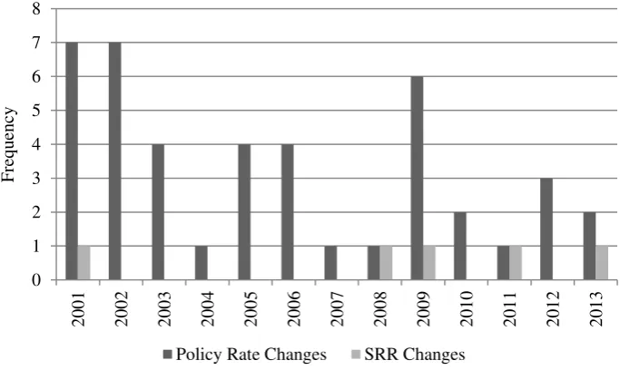
[image:10.595.142.484.348.552.2]

corridor is the main instrument used to signal the monetary policy stance of the Central Bank of Sri Lanka.

Figure 1: Frequency of Policy Interest Rate and SRR Changes 2000 - 2013

Estimating a monetary policy rule for Sri Lanka is not straightforward given the changes in the conduct of monetary policy. Although reserve money continues to be the target of monetary policy there has been a shift towards the use of the interest rate corridor to signal the stance of monetary policy. Further with the developments in financial markets there has been an improvement in the transmission of policy rates to other interest rates further

justifying the use of the interest rate as the policy instrument. Difficulties arise in estimating a monetary policy rule for Sri Lanka as it requires measuring potential output which is unobserved and could change due to structural changes taking place in the economy.

0 1 2 3 4 5 6 7 8 2 0 0 1 2 0 0 2 2 0 0 3 2 0 0 4 2 0 0 5 2 0 0 6 2 0 0 7 2 0 0 8 2 0 0 9 2 0 1 0 2 0 1 1 2 0 1 2 2 0 1 3 Fre q u en cy

(11)

10

IV. METHODOLOGY

Several alternative specifications of the policy reaction function were estimated for Sri Lanka. A contemporaneous specification of the form given in equation (1) was estimated. The estimation results are given in Annex II. In the light of Judd and Rudebusch (1998) and Rotemberg and Woodford (1999) finding that backward looking specifications of the Taylor rule are relatively good approximations of optimal policy, a backward looking specification of a monetary policy rule of the form set out in equation (2) was estimated.

(1)

where is the short term interest rate or the policy rate of the central bank, is the year on year rate of inflation, is the desired level of inflation, is the output gap, is the change in the nominal exchange rate and is a random disturbance term.

(2)

However, given the lags in the transmission of monetary policy, in practice central banks are found to be more forward looking in their decision making. Hence, a forward looking monetary specification of the policy reaction function of the form set out in equation (3) was also estimated.

(3)

In the empirical literature (Clarida et al, 2000, Paez-Farrell, 2009) the interest rate

smoothing behaviour of central banks is taken into consideration by including a lagged value of the interest rate.

Exchange rate smoothing has also been found to be an important consideration in the policy reaction function of emerging economies (Mohanty and Klau, 2004). Given Sri Lanka is a small open economy which is highly sensitive to movements in the exchange rate, a reaction function including the exchange rate was chosen as the preferred specification.

V. DATA DESCRIPTION AND EMPIRICAL RESULTS

(12)

11

Wholesale Price Index (WPI) and the GDP deflator. Since the most widely accepted measure of inflation is the CCPI, the year on year change in the CCPI, is the inflation measure used in the analysis. The desired rate of inflation has been set at 5 per cent for the entire period of analysis.9

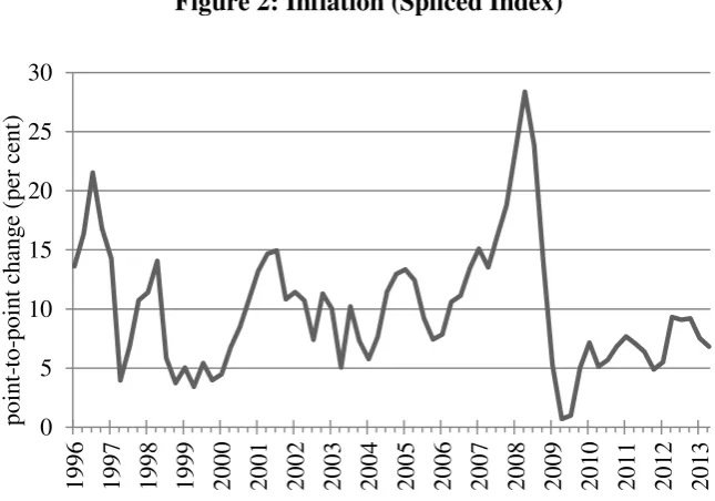
The year on year change in inflation as measured by CCPI had an average of 10.0 per cent over the sample period 1996 to 2013:Q2. The inflation gap, which is the difference between the actual inflation and the desired inflation, recorded a mean of 5.0 during the period under consideration. The descriptive statistics of the data series were also analysed by dividing the entire sample into two subsamples to evaluate the changes that have taken place since 2008. Notably, the average inflation gap during the period 2008 to 2013:Q2 was 4.09 per cent, which was lower than the average inflation gap of 5.44 per cent during the period 1996 to 2007.

[image:12.595.147.470.438.664.2]

The mean of the alternative measures of short term interest rates, namely the effective policy rate, the average weighted call market rate and the 91-day Treasury bill rate were 11.3 per cent, 11.6 per cent and 11.7 per cent respectively during the sample period 1996 to 2013:Q2. Reflecting the movement in inflation, the average interest rates have also declined during the period 2008 to 2013:Q2 from the rates prevailing during the period 1996 to. Meanwhile, the average depreciation in the exchange rate was 5.1 per cent during the entire sample period, and was also found to be lower in the latter subsample compared to the former.

Figure 2: Inflation (Spliced Index)

9_{It is recognised that this rate may not have been the Central Bank of Sri Lanka’s target rate over the entire}

sample period but it has been chosen as the target rate since the Central Bank of Sri Lanka has stated in policy documents its desires to maintain inflation at mid-single digit levels over the medium term.

0 5 10 15 20 25 30

1996 1997 1998 1999 2000 2001 2002 2003 2004 2005 2006 2007 2008 2009 2010 2011 2012 2013

poi

nt

-to

-poi

nt

cha

ng

e (

per

ce

nt

(13)

12

Measuring potential output, which cannot be observed, is one of the key issues that need to be addressed when estimating a monetary policy rule. Correctly estimating the output gap is crucial to obtaining reliable estimates of the monetary policy rule. There are several

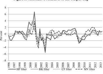
alternative methods used to estimate potential output: Univariate filtering methods such as the Hodrick Prescott filter (HP filter), Baxter King and Christiano-Fitzgerald band pass filters as well as multivariate model based methods. 10_{Alternative measures of the output}

gap for Sri Lanka based on estimates of potential output using these various methods are given in Figure 2. The figure shows a close correspondence between the alternative

[image:13.595.138.492.275.531.2]

measures of potential output. Since the potential output estimate using the HP filter measure is available for the longest period, it is chosen for the empirical analysis.

Figure 3: Alternative Measures of the Output Gap

The central bank has operated under a monetary targeting framework since the 1980s. However, since the commencement of open market operations, monetary policy has been conducted to influence the short term interest rate. Hence, the short term interest rate was

10 Hodrick-Prescott (HP) filter: Potential output represents a filter that minimises the deviation of actual output from the potential output, subject to a penalty on the maximum allowable change in potential growth between the two periods. The standard practice is to use a smoothness parameter equal to 1,600 for quarterly data. Baxter-King (BK) and Christiano-Fitzgerald (CF) band-pass filters: Accommodate business cycle dynamics using a range of business cycle frequencies to separate the cyclical and trend components of output.

Multivariate (MV) filter: A model based approach to estimating potential output. The multivariate filter is used to simulate the potential output by estimating the relationship between growth and other observable variables including inflation, capacity utilisation and unemployment.

-8 -6 -4 -2 0 2 4 6 8 1 9 9 6 1 9 9 7 1 9 9 8 1 9 9 9 2 0 0 0 2 0 0 1 2 0 0 2 2 0 0 3 2 0 0 4 2 0 0 5 2 0 0 6 2 0 0 7 2 0 0 8 2 0 0 9 2 0 1 0 2 0 1 1 2 0 1 2 2 0 1 3 P er ce n t

(14)

13

chosen to reflect the monetary policy stance of the Central Bank of Sri Lanka. Since there is no one interest rate that appropriately reflects the stance of monetary policy over the entire sample period, it was necessary to choose a short term interest rate that appropriately reflected the monetary policy stance of the Central Bank. An ‘Effective Policy Rate’ was constructed by choosing the policy interest rate that ‘best’ reflected the monetary policy stance during each period under consideration. Until the commencement of open market operations the Repo rate was considered as the effective policy interest rate. Thereafter depending on macroeconomic conditions and liquidity conditions in the market either the Repo rate or the Reverse Repo rate was chosen as the effective policy rate. To carry out robustness checks, the monetary policy rule was also estimated out using the average

[image:14.595.133.504.337.555.2]

weighted call market rate (AWCMR) the 91-day Treasury bill rate. The correlation between the AWCMR and the effective policy interest rate was found to be around 0.8, indicating the close movement between the policy interest rate and the overnight market interest rate.

Figure 4: Central Bank Policy Interest Rates and Overnight Short Term Interest Rate

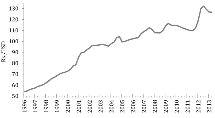
Sri Lanka being a small open economy is significantly affected by changes in its exchange rate. Hence, the exchange rate has been included in the monetary policy reaction function of the Central Bank. Following Patra and Kapur (2012) the annualised quarter on quarter change in the nominal exchange rate was used in the analysis.

0 5 10 15 20 25 30 1 9 9 6 1 9 9 7 1 9 9 8 1 9 9 9 2 0 0 0 2 0 0 1 2 0 0 2 2 0 0 3 2 0 0 4 2 0 0 5 2 0 0 6 2 0 0 7 2 0 0 8 2 0 0 9 2 0 1 0 2 0 1 1 2 0 1 2 2 0 1 3 P er ce n t

AWCMR (Quarterly Average) Repo

Reverse Repo Penal Rate

(15)

[image:15.595.127.490.111.310.2]

14

Figure 5: Rs/US dollar Exchange Rate

A Chow breakpoint stability test was carried out on a selected contemporaneous monetary policy reaction function.11_{Based on the results of the test, two statistically significant breaks}

were detected in 2001 Q1 and 2008 Q1. The break in 2001 Q1 captures the shift to a free floating exchange rate regime while the break in 2008 Q1 captures the impact of the global financial crisis. A dummy variable has been included to take into account these

extraordinary events that had an undue impact on the volatility of the short term interest rate.

Contemporaneous and backward looking models were estimated using Ordinary Least Squares (OLS). Forward looking specifications which include lead values of explanatory variables were estimated using Generalised Method of Moments (GMM) to account for possible endogeneity between variables (Clarida et al, 1998).

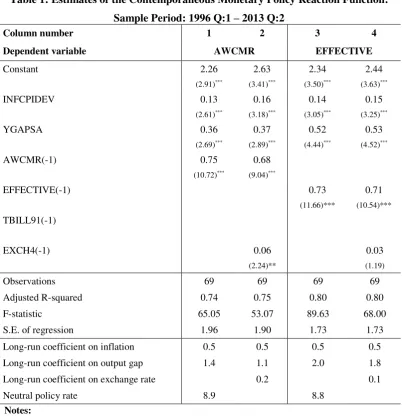
Table 1 presents a summary of the results from estimates of alternative contemporaneous specifications of the monetary policy reaction function. Two alternative measures of short term interest rate (AWCMR and the effective policy interest rate) were used in the

estimation. The baseline specifications (column 1 and 3 of Table 1) include

contemporaneous values for inflation and output gap, and the first lag of the short term interest rate to take into account interest smoothing behaviour of the central bank. The baseline specifications were augmented with the nominal exchange rate (column 2 and 4 of Table 1). Similar estimations were also carried out using the 91-day Treasury bill rate in order to perform robustness checks, and the results are given in Table 5 of Annex II.

11_{Chow breakpoint stability test can only be done for single equations, and not for a system of equations.}

Hence the break points detected are based on a contemporaneous specification of a monetary policy reaction function.

50 60 70 80 90 100 110 120 130

1996 1997 1998 1999 2000 2001 2002 2003 2004 2005 2006 2007 2008 2009 2010 2011 2012 2013

R

s./

(16)

15

[image:16.595.114.517.238.656.2]

Estimates from contemporaneous monetary policy reaction function shows that the coefficients on both inflation and output gap remain positive and significant for all specifications. The coefficient on inflation is lower than the coefficient on the output gap and the long-run coefficient on inflation is less than unity indicating that the Taylor principle is not fulfilled. The use of a contemporaneous specification which ignores the lags in the transmission of monetary policy could be the reason for this result. However, the coefficient on the output gap is above unity. The exchange rate variable is found to be significant in one of the augmented specification (column 2 of Table 1) although the coefficient is small.

Table 1: Estimates of the Contemporaneous Monetary Policy Reaction Function: Sample Period: 1996 Q:1 – 2013 Q:2

Column number 1 2 3 4

Dependent variable AWCMR EFFECTIVE

Constant 2.26 2.63 2.34 2.44

(2.91)*** _(3.41)*** _(3.50)*** _(3.63)***

INFCPIDEV 0.13 0.16 0.14 0.15

(2.61)*** _(3.18)*** _(3.05)*** _(3.25)***

YGAPSA 0.36 0.37 0.52 0.53

(2.69)*** _(2.89)*** _(4.44)*** _(4.52)***

AWCMR(-1) 0.75 0.68

(10.72)*** _(9.04)***

EFFECTIVE(-1) 0.73 0.71

(11.66)*** (10.54)***

TBILL91(-1)

EXCH4(-1) 0.06 0.03

(2.24)** (1.19)

Observations 69 69 69 69

Adjusted R-squared 0.74 0.75 0.80 0.80

F-statistic 65.05 53.07 89.63 68.00

S.E. of regression 1.96 1.90 1.73 1.73

Long-run coefficient on inflation 0.5 0.5 0.5 0.5

Long-run coefficient on output gap 1.4 1.1 2.0 1.8

Long-run coefficient on exchange rate 0.2 0.1

Neutral policy rate 8.9 8.8

Notes:

Absolute value of t-statistics is given in parentheses.

* significant at 10%; ** significant at 5%, *** significant at 1%

Estimation is by OLS methodology for the sample period 1996Q1 - 2013Q2 Output gap measure: Hodrick-Prescott filter

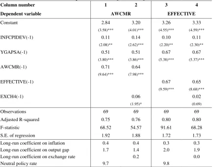
Table 2 presents a summary of the results from estimates of a backward looking

(17)

16

[image:17.595.94.529.255.597.2]

interest rate (AWCMR and the effective policy interest rate) were used to estimate the backward looking monetary policy reaction function. The baseline specifications (column 1 and 3 of Table 2) included lagged inflation and output gap, and the short term interest rate with one lag. The baseline specifications were augmented with the nominal exchange rate (column 2 and 4 of Table 2). Similar estimations were also carried out using the 91-day Treasury bill rate in order to perform robustness checks, and the results are given in Table 6 of Annex II.

Table 2: Estimates of Monetary Policy Reaction Function - Backward Looking Specifications Sample Period: 1996 Q:1 – 2013 Q:2

Column number 1 2 3 4

Constant 2.84 3.20 3.26 3.33

(3.58)*** (4.01)*** (4.55)*** (4.59)***

INFCPIDEV(-1) 0.11 0.14 0.10 0.11

(2.08)** (2.62)*** (2.20)** (2.30)**

YGAPSA(-1) 0.51 0.51 0.67 0.67

(3.80)*** (3.86)*** (5.38)*** (5.37)***

AWCMR(-1) 0.71 0.64

(9.64)*** (7.98)***

EFFECTIVE(-1) 0.67 0.65

(9.59)*** (8.68)***

EXCH4(-1) 0.06 0.02

(1.95)* (0.69)

Observations 69 69 69 69

Adjusted R-squared 0.75 0.76 0.80 0.80

F-statistic 68.52 54.57 91.61 68.28

S.E. of regression 1.92 1.88 1.72 1.73

Long-run coefficient on inflation 0.4 0.4 0.3 0.3 Long-run coefficient on output gap 1.7 1.4 2.0 1.9 Long-run coefficient on exchange rate 0.2 0.0

Neutral policy rate 9.7 9.8

Notes:

Absolute value of t-statistics is given in parentheses.

Estimation is by OLS methodology for the sample period 1996Q1 - 2013Q2 Output gap measure: Hodrick-Prescott filter

Estimates from the backward looking monetary policy reaction function show that the coefficients on both inflation and output gap remain positive and significant for all

(18)

17

The exchange rate variable turns out to be significant in one of the augmented specifications (column 2 of Table 2).

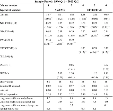
Table 3 presents a summary of the results from estimates of a forward looking specification of a monetary policy reaction function. Similar to the contemporaneous and backward looking specifications, the AWCMR and the effective policy interest rate were used as two alternative measures of short term interest rate. One quarter ahead inflation and output gap together with short term interest rate with one lag were used in the baseline specifications (column 1 and 4 of Table 3). The baseline was augmented with a dummy variable to account for the structural breaks identified in 2001 and 2008 (column 2 and 5 of Table 3). In

addition, the specifications were also augmented with movements in the nominal exchange rate (column 3 and 6 of Table 3). Robustness checks were carried out using the 91-day Treasury bill rate, and the results are given Table 7 of Annex II.

The coefficients on inflation and the output gap are statistically significant and have the right sign. However, the coefficient on the output gap is larger than the coefficient on inflation. The coefficient on lagged interest rate is large and significant implying a relatively high degree of interest rate smoothing. This indicates that the central bank generally changes its policy interest rate in small steps in response to macroeconomic developments. Increasing uncertainty of the macroeconomic environment and the monetary transmission mechanism have made central banks more cautious in the conduct of monetary policy. The long run coefficient12_{on inflation is greater than 1 in all forward looking specifications of the}

monetary policy reaction function indicating that in the forward looking specification of the monetary policy rule the Taylor principle13

is satisfied. The long run coefficient on the output gap is larger than the coefficient inflation indicating that monetary policy seems to react more strongly to fluctuations in output than to deviations in inflation. The higher coefficient on the output gap may reflect a higher preference towards output stabilisation but it could also reflect a lower sensitivity of output to the interest rate and hence the need for a stronger response of monetary policy towards output stabilisation (Hayo and Hoffman, 2005). In emerging markets and developing countries, monetary policy is supposed to react more strongly to movements in the exchange rate. In the forward looking specification the coefficient on the exchange rate is of the right sign, indicating that monetary policy is tightened in response to depreciation in the exchange rate but the coefficient is very small and not significant. According to Mohanty and Klau (2004), the strength of the monetary

12

13

(19)

18

[image:19.595.93.533.147.579.2]

policy response to the exchange rate depends on whether a central bank is able to use other instruments such as intervention in the foreign exchange market, temporary capital controls, swaps and other derivative instruments to stabilise the exchange rate.

Table 3: Estimates of Monetary Policy Reaction Function - Forward Looking Specifications Sample Period: 1996 Q:1 – 2013 Q:2

Column number 1 2 3 4 5 6

Constant 1.87 -0.91 -1.05 1.68 -0.01 -0.05

(2.01)** (-0.25) (-0.28) (1.88)* (0.00) (-0.01)

INFCPIDEV(+1) 0.29 0.36 0.42 0.28 0.29 0.31

(1.96)** (1.79)* (1.96)** (2.71)*** (2.02)** (2.11)**

YGAPSA(+1) 0.65 0.69 0.59 0.95 0.97 0.94

(1.13) (1.21) (1.03) (1.96)** (1.90)* (1.94)*

AWCMR(-1) 0.72 0.77 0.70

(7.68)*** (6.89)*** (5.60)***

EFFECTIVE(-1) 0.73 0.78 0.76

(9.12)*** (4.86)*** (4.12)***

TBILL91(-1)

EXCH4(-1) 0.06 0.02

(1.41) (0.58)

DUMMY 2.02 2.30 1.12 1.16

(0.71) (0.81) (0.35) (0.36)

Observations 68 68 68 68 68 68

Adjusted R-squared 0.62 0.57 0.57 0.61 0.60 0.60

J-statistic 0.00 0.00 0.00 0.00 0.00 0.00

S.E. of regression 2.35 2.50 2.52 2.40 2.45 2.44 Long-run coefficient on inflation 1.0 1.5 1.4 1.0 1.4 1.3 Long-run coefficient on output gap 2.3 3.0 2.0 3.6 4.5 4.0 Long-run coefficient on exchange rate 0.2 0.1

Neutral policy rate 6.6 4.8 6.3 5.1

Notes:

Absolute value of t-statistics is given in parentheses

Estimation is by GMM methodology for the sample period 1996Q1 - 2013Q2

Instruments used for GMM estimation: INFCPIDEV(-1), YGAPSA(-1), AWCMR(-1), EFFECTIVE(-1), EXCH4(-1) and DUMMY

Output gap measure: Hodrick-Prescott filter

(20)

19

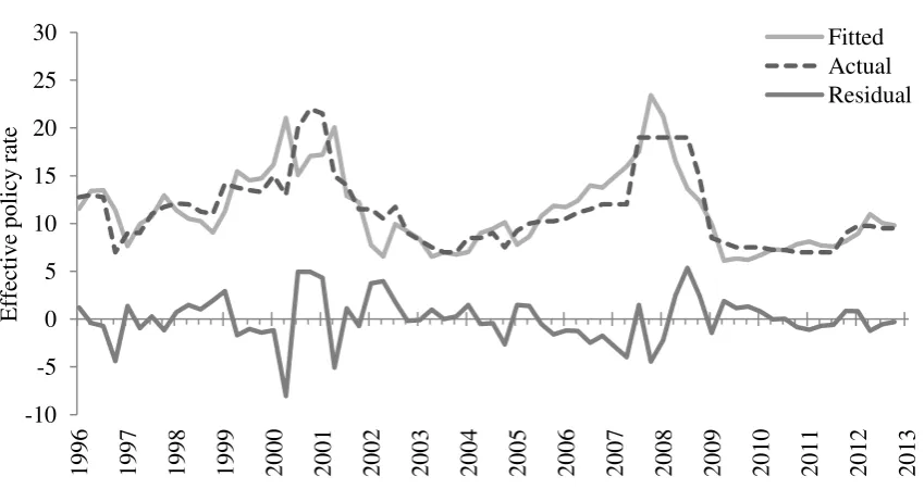
policy reaction function augmented with a dummy variable (column 5 of Table 3).14_The

[image:20.595.99.524.167.392.2]

policy interest rate estimated from the model appears to closely track the effective rate reasonably well, although there are was some deviation during 2000-2001 and 2006-2007.

Figure 6: Actual Versus Estimated Effective Policy Rate

Based on the Forward Looking Specification of the Monetary Policy Rule

Determining the neutral policy rate15_{is vital for the estimation of a monetary policy rule. It}

is possible to estimate this value using a general equilibrium model of the economy.

However, a crude estimate can be obtained from the estimation of the Taylor rule itself. The estimates of the neutral policy interest rate in the contemporaneous specification is around 8.9 per cent while for the backward looking specification it is around 9.8 per cent indicating the need for high interest rates if the lags in transmission of monetary policy are not taken into consideration by policy makers. According to estimates of forward looking

specifications of the monetary policy reaction function, the neutral policy rate is around 6.2 - 6.6 per cent. 16

Assuming a higher level of desired inflation during the first sub sample period results in a neutral policy rate estimate of between 10-11 per cent.

14_{The selected specification has a Durbin-Watson statistic of 1.77, which is approximately close to the desired}

level of 2, the level of serial correlation is not significant. According to the Ljung-Box Q-statistic the null hypothesis that there is no autocorrelation can be accepted.

15

The neutral policy rate is the policy rate at which the economy is assumed to be growing at its potential level and inflation is maintained at the desired level.

16_{However, the estimates of the neutral policy rate should be treated as indicative and within wide confidence}

intervals, as the assessment of the neutral rate is conditional upon the view on the rate of potential output growth (Patra and Kapur, 2010).

(continued…)

-10 -5 0 5 10 15 20 25 30

1996 1997 1998 1999 2000 2001 2002 2003 2004 2005 2006 2007 2008 2009 2010 2011 2012 2013

Eff

ec

ti

v

e

pol

icy

r

at

e

(21)

[image:21.595.100.530.112.345.2]

20

Figure 7: Interest Rate Gap and Inflation Gap

Figure 7 plots the interest rate gap which is the difference between the effective policy rate and the interest rate implied by the estimated monetary policy rule and the inflation gap which is the difference between the inflation rate and targeted inflation. The figure shows an inverse relationship between the interest rate gap and the inflation gap. Periods during which the actual interest rate was close to the implied rate implied by the estimated Taylor rule, actual inflation is closer to the desired/targeted rate of inflation. In periods where there is a deviation of the effective policy rate from the policy rate implied by the Taylor rule, the larger the gap between actual inflation and the desired/targeted rate of inflation. A widening gap is observed during the period 2007-2008, coinciding with the Global Financial Crisis.

A recursive regression was carried out for the backward looking specification in column 3 of Table 2 to assess the evolution of the coefficients on the inflation gap and output gap over time. The results are presented in Figure 7. According to the estimates the response of monetary policy to deviations of inflation from the desired level and the output gap has strengthened since 2007, reaching a peak in 2009. The response of monetary policy to inflation has stabilised thereafter, while the response to the output gap appears to have gradually declined reflecting the improvement in the transmission of monetary policy. The coefficient on the output gap has been consistently higher than the coefficient on the

inflation gap reflecting the lower sensitivity of output to interest rates.

Figure 8: Recursive Estimates of Coefficients of Inflation Gap and Output Gap -10 -5 0 5 10 15 20 25 -10 -8 -6 -4 -2 0 2 4 6 8 199 6 199 7 199 8 199 9 200 0 200 1 200 2 200 3 200 4 200 5 200 6 200 7 200 8 200 9 201 0 201 1 201 2 201 3 Inf lat ion Int er es t rat e

(22)

21

a. Inflation Gap

b. Output Gap

Since there appears to be a definite shift in the coefficients on inflation gap and output gap after 2007, the monetary policy reaction function was estimated over two sub sample

periods. The first sample period covered the period 1996 Q:1 to 2007 Q:4, while the second sample period was from 2008 Q:1 to 2013 Q:2. Due to insufficient number of observations in the second sample period the results from that period are not reported. However,

comparing the results from the first sample period and the entire sample provide some important insights into the changes that have taken place in the conduct of monetary policy. The long run coefficient on inflation was less than one which was below the threshold prescribed by the Taylor principle, implying that during this period monetary policy has reacted less than proportional to changes in inflation. On the other hand, for the entire sample period, the long run coefficient was above 1, indicating that during the second sample period the Taylor principle was met. With monetary policy reacting more than proportionately to the inflation gap, there is an increase in the real interest rate leading to

0.00 0.02 0.04 0.06 0.08 0.10 0.12

2003 2004 2005 2006 2007 2008 2009 2010 2011 2012 2013

C

oef

fi

ci

ent

of

i

nf

lat

ion

g

ap

0.55 0.60 0.65 0.70 0.75

2003 2004 2005 2006 2007 2008 2009 2010 2011 2012 2013

C

oef

fi

ci

ent

of

out

put

g

(23)

22

[image:23.595.90.547.181.516.2]

lower inflation. Further the long run coefficient on output gap is higher during the second period indicating a higher weight on output stabilisation.

Table 4: Estimates of Monetary Policy Reaction Function - Forward Looking Specifications Sample Periods: 1996:Q1 to 2007:Q4 and 1996 Q:1 to 2013 Q:2

Sample period 1996Q1 2007Q4 1996Q1 2013Q2

Constant 2.28 9.52 9.53 1.68 -0.01 -0.05

(1.43) (1.55) (1.52) (1.88)* (0.00) (-0.01) INFCPIDEV(+1) 0.28 0.26 0.26 0.28 0.29 0.31

(1.46) (1.59) (1.63) (2.71)*** (2.02)** (2.11)**

YGAPSA(+1) 1.18 1.17 1.15 0.95 0.97 0.94

(1.86)* (1.96)* (1.98)** (1.96)** (1.90)* (1.94)* EFFECTIVE(-1) 0.68 0.42 0.36 0.73 0.78 0.76

(6.29)*** (1.65) (1.26) (9.12)*** (4.86)*** (4.12)***

EXCH4(-1) 0.06 0.02

(1.25) (0.58)

DUMMY -4.50 -4.20 1.12 1.16

(-1.07) (-1.00) (0.35) (0.36)

J-statistic 0.00 0.00 0.00 0.00 0.00 0.00

S.E. of regression 2.86 2.79 2.76 2.40 2.45 2.44

Long-run coefficient on inflation 0.9 0.4 0.4 1.0 1.4 1.3 Long-run coefficient on output gap 3.6 2.0 1.8 3.6 4.5 4.0

Long-run coefficient on exchange rate 0.1 0.1

Neutral policy rate 7.0 8.7 6.3 5.1

Notes:

* significant at 10%; ** significant at 5%, *** significant at 1% Estimation is by GMM methodology for the effective interest rate

Instruments used for GMM estimation: INFCPIDEV(-1), YGAPSA(-1), AWCMR(-1), EFFECTIVE(-1), EXCH4(-1) and DUMMY

Output gap measure: Hodrick-Prescott filter

VI. CONCLUSION

The paper provides an empirical characterisation of the monetary policy reaction function of the Central Bank of Sri Lanka over the period 1996Q1 to 2013Q2. . Although the

objectives of the Central Bank have changed during this period as have its operating methods, the monetary policy stance of the Central Bank appears to have been well

(24)

23

by the Central Bank on inflation and output during the period for which the analysis was conducted.

The estimates provide evidence of a change in the coefficients for the inflation gap and the output gap during the period of analysis, in particular with a stronger response of monetary policy to the inflation gap and the output gap being observed since 2007. There is also evidence of a greater weight being placed on output stabilisation, which could reflect both the preference of the central bank and structural issues relating to the slower transmission of monetary policy. A relatively strong response to the output gap may be attributed to a lower sensitivity of output to the interest rate. However, there appears to be a shift in monetary policy from greater responsiveness to the output gap to more focus on inflation. The empirical analysis however, does not provide any evidence that monetary policy is responsive to the exchange rate.

The challenges discussed previously in the estimation of monetary policy reaction functions were encountered in the case of Sri Lanka as well. Generating reliable estimates of potential output is particularly challenging given the structural changes that have taken place in the economy. Difficulties also arise in determining the equilibrium real interest rate which may therefore give rise to policy error. Further identifying a single targeted or desired inflation rate for the entire period of the analysis is challenging.

Taylor type monetary policy rules provide a simple and transparent framework for

(25)

References

Ball, Laurence, 1999. “Policy rules for open economies”, in John B Taylor (ed), Monetary policy rules, NBER, 127-56.

Batini, Nicoletta and Andrew G Haldane, 1999. “Forward-Looking Rules for Monetary

Policy,” In Taylor, J.B. (ed.), Monetary Policy Rules. University of Chicago Press: Chicago.

Beck, Guenter and Wieland, Volker, 2008. "Central bank misperceptions and the role of money in interest rate rules," Working Paper Research 147, National Bank of Belgium.

Blinder, Alan, 2006. "Monetary Policy Today: Sixteen Questions and about Twelve

Answers," Working Papers 73, Princeton University, Department of Economics, Center for Economic Policy Studies.

Clarida, Richard, Jordi Gali and Mark Gerlter. 1998. “Monetary Policy Rules in Practice:

Some International Evidence”, European Economic Review, 42, 1033-1067.

Clarida, Richard, Jordi Gali and Mark Gerlter. 1999 “The Science of Monetary Policy: A

New Keynesian Perspective”, Journal of Economic Literature, Vol. 37 (4), 1661-1707.

Clarida, Richard, Jordi Gali and Mark Gerlter. 2000. “Monetary Policy Rules and

Macroeconomic Stability”, Quarterly Journal of Economics, 115, 147-180.

Dattels, Peter and others. 2001. Sri Lanka: “A Strategy for Strengthening the Framework and

Implemenation of Monetary and Foreign Exchange Operations.” Technical Assistance

Report, International Monetary Fund, Washington D.C.

Debabrata, Michael Patra and Muneesh Kapur. 2010, “A Monetary Policy Model without

Money for India” IMF Working Paper WP/10/183.

English, William, William Nelson and Brian Sack. 2003, “Interpreting the Significance of the Lagged Interest Rate in Estimated Monetary Policy Rules” Contributions to Macroeconomics Vol 3(1).

Gali, Jordi and Mark Gertler, 2007. “Macroeconomic Modelling for Monetary Policy Evaluation”, Journal of EconomicmPerspectives, 21(4), 25-45.

Judd, John P and Glenn D. Rudebusch, 1998. “Taylor’s Rule and the Fed: 1970-1997,” Federal Reserve Bank of San Francisco Economic Review, no.3, 3-16.

(26)

25

Lowe, Philip and Luci Ellis, 1997. “The smoothing of official interest rates”, Monetary policy and inflation targeting, Reserve Bank of Australia, 287-312.

McCallum, B.T., 1999. “Recent Developments in the Analysis of Monetary Policy Rules”, Homer Jones memorial Lecture, March 11, 1999, 11.

McCallum, B.T., 2000. “Alternative Monetary Policy Rules: A Comparison with Historical Settings for the United States, the United Kingdom, and Japan," Working Paper 7725, National Bureau of Economic Research.

Mohanty, M.S. and Marc Klau, 2004. “Monetary Policy Rules in Emerging Market Economies: Issues and Evidence”, Bank of International Settlements Working Paper No. 149.

Orphanides, A. and S. van Norden, 1999. The Reliability of Output Gap Estimates in Real-Time, Board of Governors of the Federal Reserve System Finance and Economics

Discussion Series No. 38

Orphanides, Athanasios, 2001. “Monetary policy rules, macroeconomic stability and

inflation: a view from the trenches,” Finance and Economics Discussion Series 2001-62, Board of Governors of the Federal Reserve System.

Orphanides, Athanosios, 2003. “Historical Monetary Policy Analysis and the Taylor Rule”,

Journal of Monetary Economics, 50(5), 983-1022.

Orphanides, Athanosios, 2007. “Taylor Rules”, Working Paper FEDS 2007-18, Board of

Governors of the Federal Reserve System, January.

Paez-Farrell, Juan, 2009. “Monetary Policy Rules in Theory and Practice: Evidence from the

UK and US”, Applied Economics, 4(16), 2037-2046.

Rotemberg, Julio J., and Michael Woodford, 1999. “Interest Rules in an Estimated Sticky Price Model”, in John B. Taylor (ed.), 1999, Monetary Policy Rules, University of Chicago Press, Chicago, 57-126.

Sack, Brian and Volker Wieland, 1999. “Interest-Rate Smoothing and Optimal Monetary

Policy: A Review of Recent Empirical Evidence,” Finance and Economics Discussion Series,

1999-39, Federal Reserve Board, (August).

(27)

26

Svensson Lars E O, 2002. “Inflation targeting: should it be modelled as an instrument rule or a target rule”. European Economic Review, 46, 771-80.

Svensson Lars E O, 2003. “Escaping from a Liquidity Trap: The Foolproof Way and

Others”, Journal of Economic perspectives, Vol. 17(4), 145-66.

Taylor, John B., 1993. “Discretion versus Policy Rules in Practice”, Carnegie-Rochester Conference Series on Public Policy, 39, 195-214.

Taylor, John B., 1999. “A Historical Analysis of Monetary Policy Rules” in John B. Tayloe

(ed.), “Monetary Policy Rules”, University of Chicago Press, Chicago, 319-348.

Taylor, John B., 2002. “Using Monetary Policy Rules in Emerging Market Economies”

Stabilisation and Monetary Policy, Banco de Mexico, 441-57.

Taylor, John B. and John C. Williams, 2010. “Simple and Robust Rules for Monetary Policy”, National Bureau of Economic Research Working Paper No. 15908.

Wijesinghe, D.S. 2006. “Active Open Market Operations”, Staff Studies Central Bank of Sri

Lanka , 36(1 & 2), 15-35.

(28)

27

[image:28.612.85.541.113.448.2]

Annex I

Table 1: Data Description

Variable Name Definition Period Source

AWCMR Average weighted call money rate

(quarterly average) 1996 – 2013:Q2 CBSL

1

EFFECTIVE Effective policy rate 1996 - 2012:Q2 CBSL

TBILL91 91 day Treasury bill rate 1996 - 2012:Q2 CBSL

EXCH4 Annualised quarter-on-quarter variation in

the monthly average exchange rate 1996 - 2012:Q2 CBSL

INFCPIDEV

Deviation of actual inflation (change of

the Colombo Consumers’ Price Index

(CCPI)) from the indicative inflation projection of 5 per cent

1996 - 2012:Q2

DCS2

Author’s

estimates

YGAPSA Output gap measure (computed using

seasonally adjusted GDP) 1996 - 2012:Q2

Author’s

estimates

DUMMY 2001:Q1-Q3 and 2008:Q1-Q3 are set to 0 - -

1/ CBSL – Central Bank of Sri Lanka

2/ DCS – Department of Census and Statistics, Sri Lanka

Table 2: Sylised Facts (Averge for Period)

Per cent

Period

Headline Inflation (CCPI)

Real GDP Growth Rate

(YRATE)

Output Gap (YGAPSA

Average Weighted Call Market

Rate (AWCMR)

Depreciation of Rs/US $

Exchange Rate (EXCH4) 1996-2013Q2 10.0 5.2 0.0 11.6 5.1

1996-2001 10.1 4.0 0.7 14.5 9.3

2002-2007 10.8 5.4 -0.6 10.8 3.1

2008-2013Q2 9.1 6.4 -0.1 9.5 2.6

[image:28.612.85.550.447.677.2]

(29)

28

[image:29.612.91.559.126.423.2]

Table 3: Descriptive Statistics

Table 3.1: Descriptive Statistics: 1996 – 2013

AWCMR EFFECTIVE TBILL91 EXCH4 INFCPIDEV YGAPSA

Mean 11.64 11.31 11.69 5.07 5.02 -0.01

Median 11.05 10.50 11.29 5.15 4.20 -0.20

Maximum 23.83 22.00 21.30 37.50 23.40 6.68

Minimum 7.02 7.00 6.98 -18.90 -4.30 -5.57

Std. Dev. 3.80 3.82 3.67 8.98 5.34 1.78

Skewness 1.24 1.11 0.72 1.00 1.05 0.41

Kurtosis 4.57 3.62 2.67 6.21 4.42 5.59

Jarque-Bera 25.00 15.46 6.43 41.83 18.76 21.57

Probability 0.00 0.00 0.04 0.00 0.00 0.00

Sum 814.47 791.46 818.13 355.10 351.10 -0.51

(30)

29

Table 3.2 Descriptive Statistics: 1996 – 2007

Mean 12.63 11.72 12.13 6.21 5.44 0.05

Median 12.27 11.50 11.79 5.65 5.75 -0.20

Maximum 23.83 22.00 21.30 35.40 16.50 6.68

Minimum 7.48 7.00 7.00 -18.90 -1.60 -5.57

Std. Dev. 3.88 3.45 3.56 7.54 4.29 1.98

Skewness 1.18 1.25 0.72 0.54 0.23 0.44

Kurtosis 4.27 4.75 2.92 8.24 2.52 5.19

Jarque-Bera 14.39 18.70 4.11 57.35 0.88 11.14

Probability 0.00 0.00 0.13 0.00 0.65 0.00

Sum 606.03 562.71 582.34 298.20 261.10 2.32

[image:30.612.85.560.418.726.2]

Sum Sq. Dev. 706.11 559.17 595.92 2674.85 863.91 184.57

Table 3.3: Descriptive Statistics: 2008 – 2013

Mean 9.47 10.40 10.72 2.59 4.09 -0.13

Median 8.48 8.75 9.48 -0.60 1.95 0.04

Maximum 15.09 19.00 18.39 37.50 23.40 1.72

Minimum 7.02 7.00 6.98 -10.60 -4.30 -2.49

Std. Dev. 2.57 4.48 3.80 11.32 7.17 1.28

Skewness 1.17 1.25 0.93 1.68 1.60 -0.40

Kurtosis 2.86 2.88 2.48 5.61 4.58 2.02

Jarque-Bera 5.02 5.74 3.45 16.63 11.64 1.46

Probability 0.08 0.06 0.18 0.00 0.00 0.48

Sum 208.44 228.75 235.79 56.90 90.00 -2.83

(31)

[image:31.612.126.507.122.295.2]

30

Table 4: Unit Root Tests

Variable

Augmented Dickey-Fuller test statistic

t-Statistic Probability

AWCMR -2.88983 0.0518

EFFECTIVE -2.33379 0.1645

TBILL91 -2.64335 0.0895

EXCH4 -5.06895 0.0001

INFCPIDEV -3.92929 0.0031

(32)

31

[image:32.612.90.545.152.625.2]

Annex II

Table 5: Estimates of the Contemporaneous Monetary Policy Reaction Function

Dependent variable AWCMR EFFECTIVE TBILL91

Constant 2.26 2.63 2.34 2.44 1.74 1.98

(2.91)*** _(3.41)*** _(3.50)*** _(3.63)*** _(2.93)*** _(3.34)***

INFCPIDEV 0.13 0.16 0.14 0.15 0.11 0.13

(2.61)*** _(3.18)*** _(3.05)*** _(3.25)*** _(2.79)*** _(3.30)***

YGAPSA 0.36 0.37 0.52 0.53 0.41 0.42

(2.69)***

(2.89)***

(4.44)***

(4.52)***

(4.38)***

(4.57)***

AWCMR(-1) 0.75 0.68

(10.72)***

(9.04)***

EFFECTIVE(-1) 0.73 0.71

(11.66)***

(10.54)***

TBILL91(-1) 0.80 0.75

(14.28)***

(12.59)***

EXCH4(-1) 0.06 0.03 0.04

(2.24)**

(1.19) (1.98)**

F-statistic 65.05 53.07 89.63 68.00 137.94 109.07

S.E. of regression 1.96 1.90 1.73 1.73 1.39 1.36

Long-run coefficient on

inflation 0.5 0.5 0.5 0.5 0.5 0.5

output gap 1.4 1.1 2.0 1.8 2.1 1.7

exchange rate 0.2 0.1 0.2

Neutral policy rate 8.9 8.8 8.8

Notes:

* significant at 10%; ** significant at 5%, *** significant at 1% Estimation method: OLS

(33)

[image:33.612.89.544.97.568.2]

32

Table 6: Estimates of the Backward Looking Monetary Policy Reaction Function

Constant 2.84 3.20 3.26 3.33 2.44 2.68

(3.58)***

(4.01)***

(4.55)***

(4.59)***

(3.91)***

(4.24)***

INFCPIDEV(-1) 0.11 0.14 0.10 0.11 0.11 0.13

(2.08)**

(2.62)***

(2.20)**

(2.30)**

(2.79)***

(3.23)***

YGAPSA(-1) 0.51 0.51 0.67 0.67 0.49 0.49

(3.80)***

(3.86)***

(5.38)***

(5.37)***

(5.04)***

(5.13)***

AWCMR(-1) 0.71 0.64

(9.64)*** _(7.98)***

EFFECTIVE(-1) 0.67 0.65

(9.59)*** _(8.68)***

TBILL91(-1) 0.74 0.69

(12.22)*** _(10.60)***

EXCH4(-1) 0.06 0.02 0.03

(1.95)*

(0.69) (1.69)*

F-statistic 68.52 54.57 91.61 68.28 141.91 110.20

S.E. of regression 1.92 1.88 1.72 1.73 1.37 1.36

inflation 0.4 0.4 0.3 0.3 0.4 0.4

output gap 1.7 1.4 2.0 1.9 1.9 1.6

exchange rate 0.2 0.0 0.1

Notes:

* significant at 10%; ** significant at 5%, *** significant at 1% Estimation method: OLS

(34)

[image:34.612.50.590.84.633.2]

33

Table 7: Estimates of the Forward Looking Monetary Policy Reaction Function

Column number 1 2 3 4 5 6 7 8 9 10 11 12 13

Constant 1.87 -0.91 2.12 -1.05 1.68 -0.01 1.71 1.88 -0.05 1.96 -2.40 2.35 -2.34

(2.01)** (-0.25) (2.20)** (-0.28) (1.88)* (0.00) (1.88)* (2.10)** (-0.01) (1.63) (-0.72) (1.46) (-0.65)

INFCPIDEV(+1) 0.29 0.36 0.34 0.42 0.28 0.29 0.30 0.25 0.31 0.34 0.44 0.42 0.52

(1.96)** (1.79)* (2.44)** (1.96)** (2.71)*** (2.02)** (2.72)*** (3.41)*** (2.11)** (3.45)*** (2.34)** (2.81)*** (2.02)**

YGAPSA(+1) 0.65 0.69 0.52 0.59 0.95 0.97 0.92 1.01 0.94 0.57 0.66 0.45 0.55

(1.13) (1.21) (0.93) (1.03) (1.96)** (1.90)* (1.98)** (1.94)* (1.94)* (1.65)* (1.61) (1.20) (1.30)

AWCMR(-1) 0.72 0.77 0.64 0.70

(7.68)*** (6.89)*** (5.93)*** (5.60)***

EFFECTIVE(-1) 0.73 0.78 0.71 0.72 0.76

(9.12)***_(4.86)***_(7.72)***_(8.21)***_(4.12)***

TBILL91(-1) 0.68 0.77 0.60 0.70

(5.54)*** (5.39)*** (2.89)*** (3.09)***

EXCH4(-1) 0.06 0.06 0.03 0.02 0.05 0.05

(1.52) (1.41) (0.77) (0.58) (1.10) (0.95)

REER(-1) 0.03

(0.48)

DUMMY 2.02 2.30 1.12 1.16 3.14 3.36

(0.71) (0.81) (0.35) (0.36) (1.16) (1.23)

Observations 68 68 68 68 68 68 68 68 68 68 68 68 68

Adjusted R-squared 0.62 0.57 0.63 0.57 0.61 0.60 0.62 0.60 0.60 0.72 0.65 0.69 0.60

J-statistic 0.00 0.00 0.00 0.00 0.00 0.00 0.00 0.00 0.00 0.00 0.00 0.00 0.00

S.E. of regression 2.35 2.50 2.33 2.52 2.40 2.45 2.39 2.45 2.44 1.96 2.20 2.07 2.35

Long-run coefficient

on inflation 1.0 1.5 1.0 1.4 1.0 1.4 1.0 0.9 1.3 1.1 1.9 1.0 1.7 Long-run coefficient

on output gap 2.3 3.0 1.5 2.0 3.6 4.5 3.1 3.6 4.0 1.8 2.9 1.1 1.8 Long-run coefficient

on exchange rate 0.2 0.2 0.1 0.1 0.1 0.1 0.2

Notes:

* significant at 10%; ** significant at 5%, *** significant at 1% Estimation method: GMM

Instruments used for GMM estimation: INFCPIDEV(-1), YGAPSA(-1), AWCMR(-1), EFFECTIVE(-1), TBILL91(-1), EXCH4(-1) and DUMMY