Exact Solution for a Class of Stiff Systems by Differential Transform Method

Exact Solution for a Class of Stiff Systems by Differential

Transform Method

Muhammad Idrees1, Fazle Mabood2*, Asar Ali3, Gul Zaman4 1_{City University of Science and Information Technology, Peshawar, Pakistan}

2_{Department of Mathematics, Edwardes College, Peshawar, Pakistan}

3_{Department of Electrical Engineering, City University of Science and Information Technology, Peshawar, Pakistan} 4_{Department of Mathematics, University of Malakand, Chakdara Dir (Lower), Pakistan}

Email: [email protected], *_{[email protected], [email protected], [email protected]} Received November 22, 2012; revised February 1, 2013; accepted February 8, 2013

ABSTRACT

In this paper, Differential Transform Method (DTM) is proposed for the closed form solution of linear and non-linear stiff systems. First, we apply DTM to find the series solution which can be easily converted into exact solution. The method is described and illustrated with different examples and figures are plotted accordingly. The obtained result confirm that DTM is very easy, effective and convenient.

Keywords: Differential Transform Method; Stiff System; Inverse Differential Transform

1. Introduction

Consider the stiff initial value problem [1]:

 



,

 



,

 

0

y x  f x x y x y₀ (1)

on the finite intervalI



x x0, N



, where



0



: , m

N

y x x R and



₀



m N

: , m

f x x R R are con- tinuous.

The initial value problem of stiff differential equations occurs in almost every field of science [1-5], particularly, in the fields of:

1) Chemical Reactions: A famous chemical reaction is the Oregenator reaction between HBrO2, Br−, and Ce (IV) described by Field and Noyes in 1984.

2) Reaction-diffusion systems: Problems in which the diffusion is modeled via the Laplace operator may be- come stiff as they are discretized in space by finite dif- ferences or finite elements. Well-known example of such systems which appear so often in mathematical biology.

Several further occurrences of stiffness can be found in electrical circuits, mechanics, meteorology, oceanog- raphy and vibrations.

Definition 1: If the solution of the system contains

components which change at significantly different rates for given changes in the independent variable, then sys- tem is said to be stiff [2,3].

Stiff differential equations are characterized as those whose exact solution has a term of the form et_{, where}

 is a large positive constant. The key features of stiff equations are that the derivative terms may increase rap- idly as t increases [1].

In the last three decades numerous works have been focusing on the development of more advanced and effi- cient methods for stiff problems [1,2]. The situation be- comes more complicated when stiffness coupled with non- linearity. Carroll presents an exponential fitted scheme for solving stiff systems of initial value problems [3]. The numerical solution of linear and nonlinear system of stiff system can be found in [4-6].

Differential Transform Method (DTM) is a semi nu- merical method which gives series solution. But some- times the series solution can be easily converted into closed form solution. This Method was first introduced by Zhou [7] who solved linear and non-linear problems in electrical circuit problems. After that the method be- come very popular to solved different kind of problems. The year wise detail of such problems is as follows.

In [8], two dimensional DTM is used to solve partial differential equations (PDEs). In [9], one dimensional DTM is applied to solve linear and nonlinear initial value problems. In [10], one and two dimensional DTM has been applied to solve eigenvalue problems and PDEs. In [11], two dimensional DTM is applied to solve initial value problems for PDEs. In [12], DTM is used to solve parameters identification problems. In [13], DTM was applied to transient advective-dispersive transport equa- tion. In [14] used one dimensional DTM to solve dif- ferential-algebraic equations. In [15], three dimensional

DTM is used to solve linear and nonlinear PDEs. In [16], generalized DTM is used to solve PDEs. In [17,18], DTM is used to solve boundary value problems for inte- gro-differential equations. In [19], different approximate methods has been used for initial value problems. In [20], two dimensional DTM is utilized to solve linear and non- linear PDEs. In [21], DTM is used to solve free vibra- tions equations of beam on elastic soil. In [22], DTM is applied to solve difference equations. In [23], DTM is applied to solve differential-difference equations. In [24, 25], Generalized DTM is used to solve multi order frac- tional differential equations and linear PDEs of fractional order respectively. In [26], DTM is used to solve fourth order boundary value problem. In [27], two dimensional DTM is used to solve non-linear oscillatory system. In [28], Idrees et al. has applied DTM for the exact solution

of Goursat Problems, in [29] the authors have utilized an efficient method for stiff system, whilst in [30] the au- thors presented the numerical solution of the stiff system.

In this paper, we solve the linear and non-linear stiff system via DTM. In Section 2, we give some basic pro- perties of one-dimensional DTM. In Section 3, we have applied the method to linear and non-linear stiff systems.

2. One-Dimensional Differential Transform

In this section, we first give some basic properties of one-dimensional differential transform method. Differen- tial transform of a function y x

 

is defined as follows:

 

0 1 d

! d

k k

x

y Y k

k x _

 , (2)

where y x

 

is the original function and is the transformed function for . The differential inverse transform of is defined as

 

Y k 0,1,2,3,

k 





Y k

 

 

0

k

k

y x x Y







k



. (3) From Equations (2) and (3) we get

 

0 ₀

d ! d

k k

k

k _x

x y

y x

k x



 _





, (4)

which implies that the concept of DTM is derived from Taylor series expansion, but the method does not eva- luate the derivative symbolically. However, relative deri- vatives are calculated by an iterative procedure which is described by the transformed equations of the original functions.

In this work, we use the lower case letters to represent the original functions and upper case letters to represent the transformed functions. In actual applications, the function y x

 

is expressed by a finite series Equation (5) can be written as

 

 

0

n k

k

y x x Y







k . (5) Here is represented the convergence of natural fre- quency.

n

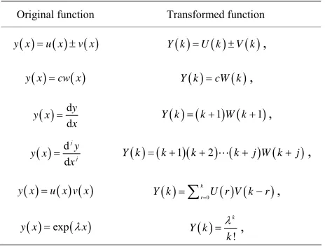
From Equations (2) and (3) we obtain Table 1 of the

fundamental operations of one-dimensional differential transform method is given by.

3. Application to Stiff System

In this section, we apply DTM to both linear and non- linear stiff systems.

Problem 1: Consider the linear stiff system:

1 1 15 2 15e

x

y   y y   , (6)

2 15 1 2 15e

x

y  y y   , (7) with initial value y₁

 

0 1, y₂

 

0 1

This system has eigen values of large modulus lying closed to the imaginary axis 1 15  I .

By applying Differential Transformation, we have





 

 

 

1 1 2

1 1

1 15 1

1 !

k

Y k Y k Y k

k 5 k

 _ 

 

    

 _ _, (8)





 

 

 

2 1 2

1 1

1 15 15

1 !

k

Y k Y k Y k

k k

 _ 

 

   

 _ _. (9)

The initial conditions of Differential Transformation are given by:

 

 

1 0 1, 2 0 1

Y  Y  .

For k0,1,2,3,, the series coefficients for Y k1

 

[image:2.595.308.540.557.733.2]

and Y k2

 

can be obtained as

Table 1. The fundamental operations of one-dimensional DTM.

Original function Transformed function

     

y x u x v x Y k U k V k ,

   

y x cw x Y k cW k ,

  d_dy y x

x

 Y k   k1 W k1,

  d_djj y y x

x

 Y k   k1k2  kj W k  j,

     

y x u x v x Y k 



_rk_0U r V k   r,

  exp 

y x  x  

!

k Y k

k



 

 

 

 

 

 

1 1 1

1 1 1

1

0 1, 1 1, 2 ,

2!

1 1 1

3 , 4 , 5 ,

3! 4! 5!

Y Y Y

Y Y Y

   

     .

 

 

 

 

 

 

2 2 2

2 2 2

1

0 1, 1 1, 2 ,

2!

1 1 1

3 , 4 , 5 ,

3! 4! 5!

Y Y Y

Y Y Y

   

     .

We used MATHEMATICA to calculate the unknown coefficients Y k1

 

and Y k2

 

.

Using the inverse Transform, we get

 

 

0

k

k

y x x Y k









, (10)

 

2 3 4 5

1 1

1! 2! 3! 4! 5!

x x x x x

y x       , (11)

 

2 3 4 5

2 1

1! 2! 3! 4! 5!

x x x x x

y x       . (12)

Equations (10) and (11) can be written in the exponen- tial form are given by

 

1 e

x

y x   , (13)

and

 

2 e

x

y x   . (14)

Thus we get the exact solution by differential trans- form method.

Problem 2: Consider the non-linear system in the

form of initial value problems [1] is given by:

 

2

1 1002 1 1000 ,2 1 0 1

y   y  y y  , (15)

 

2 2 1 2 2, 2 0

y  y y y y 1. (16)

Applying Differential Transform, we have









 

  



1

1 1 1

0 1 1 1002 1000 1 k r Y k

Y k Y r Y k r

k 



 

 _   _

 





, (17)







  

 

  



2

1 2 1 1

0 1 1 1 k r Y k

Y k Y k Y r Y k r

k      _   _  



  n

. (18)

For the series coefficients for and can be obtained as

0,1,2,3, ,

k 

 

2 Y k

 

1 Y k

 

 

 

 

 

1 1 1

1 1

0 1, 1 2, 2 2

4 2

3 , 4 , .

3 3

Y Y Y

Y Y

   

    

 

 

 

 

 

 

2 2 2

2 2 2

1

0 1, 1 1, 2 ,

2

1 1 1

3 , 4 , 5 ,

3! 4! 5!

Y Y Y

Y Y Y

   

     .

We used MATHEMATICA to calculate the unknown coefficients Y k₁

 

andY k₂

 

.

Using the inverse Transform:

 

 

0

k

k

y x x Y









k , (19)

 

2 3 4

1

2 4 8 16

1

1! 2! 3! 4!

x x x x

y x      , (20)

 

2 3 4 5

2 1 _{1! 2! 3! 4! 5!}

x x x x x

y x       . (21)

This can be written as folows

 

2

1 e

x

y x   (22)

and

 

2 e

x

y x   (23)

Thus we get the exact solution by differential trans- form method.

Problem 3: Consider the system of initial value pro-

blems[29]:

1

y  y1 (24) 2 10

y   y2 (25) 3 100

y   y3 (26) 4 1000

y   y4 (27) with initial conditions yi

 

0 1, i = 1, 2, 3, 4.

Applying Differential Transform, we have





_

1

 

_

1 1 1 Y k Y k k     ;





_

2

 

_

2 10 1 1 Y k Y k k     ;





_

3

 

_

3 100 1 1 Y k Y k k     ;





_

4

 

_

4 1000 1 1 Y k Y k k     .

With the transformed initial conditions are Yi

 

0 1, 1,2,3,4

i .

,

For k0,1,2,3, the series coefficients for Y k1

 

,

 

2

 

 

 

 

 

1 1 1

1 1

1 1

1 1, 2 , 3

2 6

1 1

4 , 5 ,

24 120

Y Y Y

Y Y

    

   

,

 

 

 

 

 

2 2 2

2 2

500

1 10, 2 50, 3 ,

3

1250 2500

4 , 5 ,

3 3

Y Y Y

Y Y

    

   

 

 

 

 

 

3 3 3

3 3

500000

1 100, 2 5000, 3 ,

3 12500000 250000000

4 , 5

3 3

Y Y Y

Y Y

    

   ,

 

 

 

 

 

4 2 4

4 4

500000000

1 1000, 2 500000, 3 ,

3 125000000000 25000000000000

4 , 5 ,

3 3

Y Y Y

Y Y

    

  

Using the inverse Transform:

 

 

0

, for 1, 2,3, 4

k

i i

k

y x x Y k i









 (28)

We obtain

1 e

x

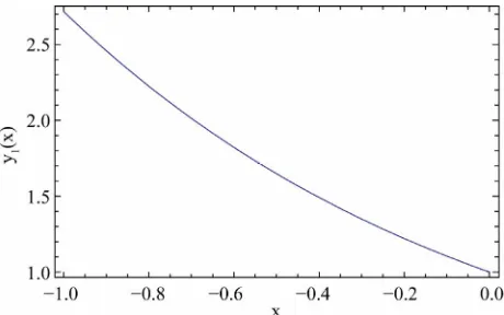
y   , y₁e10x, y₁e100x, y₁e1000x. In this section, we have presented three different linear and nonlinear stiff systems via Differential Transform Method and the series solution of Equations (13) and (22) have shown in Figures 1 and 2 respectively.

4. Conclusion

[image:4.595.310.541.84.232.2]

In this work,DTM has been applied to the exact solution of linear and non-linear stiff system. DTM is a semi nu- merical method and we obtained a closed form solution such as [11] and expressed the series form solutions in graphical form for the first two examples. It has been

Figure 1. Graphical solution of Equation (13) via DTM.

Figure 2. Graphical solution of Equation (22) via DTM.

observed that DTM is simpler, effective and reliable.

REFERENCES

[1] G. Hojjati, M. Y. Rahimi Arabili and S. M. Hosseini, “An Adaptive Method for Numerical Solution of Stiff System of Ordinary Differential Equations,” Mathematics and Computers in Simulation, Vol. 66, No. 1, 2004, pp. 33-41. doi:10.1016/j.matcom.2004.02.019

[2] E. Harier and G. Wanner, “Solving Ordinary Differential Equations II, Stiff and Differential-Algebraic Problems,” Springer-Verlag, New York, 1996.

doi:10.1007/978-3-642-05221-7

[3] L. Lopidus and W. E. Schiesser, “Numerical Methods for Differential Systems,” Academic Press, New York, 1976. [4] J. Carroll, “A Metrically Exponentially Fitted Scheme for

the Numerical Solution of Stiff Initial Value Problems,” Computers & Mathematics with Applications, Vol. 26, 1993, pp. 57-64. doi:10.1016/0898-1221(93)90034-S [5] C. H. Hsiao, “Haar Wavelet Approach to Linear Stiff

Systems,” Mathematics and Computer in Simulation, Vol. 64, No. 1, 2004, pp. 561-567.

doi:10.1016/j.matcom.2003.11.011

[6] C. H. Hsiao and W. J. Wang, “Haar Wavelet Approach to Non-Linear Stiff Systems,” Mathematics and Computer in Simulation, Vol. 57, No. 6, 2001, pp. 347-353. doi:10.1016/S0378-4754(01)00275-0

[7] J. K. Zhou, “Differential Transformation and Its Applica- tions for Electrical Circuits,” Huazhong University Press, Wuhan, 1986 (in Chinese).

[8] C. K. Chen and S. H. Ho, “Solving Partial Differential Equations by Two-Dimensional Differential Transform Method,” Applied Mathematics and Computation, Vol. 106, No. 2-3, 1999, pp. 171-179.

doi:10.1016/S0096-3003(98)10115-7

[9] M. J. Jang, C. L. Chen and Y. C. Liu, “Two-Dimensional Differential Transform for Partial Differential Equations,” Applied Mathematics and Computation, Vol. 121, No. 2-3, 2001, pp. 261-270. doi:10.1016/S0096-3003(99)00293-3 [10] I. H. Abdel-Halim Hassan, “Different Applications for the

[image:4.595.58.288.570.714.2]

No. 2-3, 2002, pp. 183-201. doi:10.1016/S0096-3003(01)00037-6

[11] F. Ayaz, “On the Two-Dimensional Differential Trans- form Method,” Applied Mathematics and Computation, Vol. 143, No. 2-3, 2003, pp. 361-374.

[12] M. J. Jang, J. S. Wang and Y. C. Liu, “Applying Differ- ential Transformation Method to Parameter Identification Problems,” Applied Mathematics and Computation, Vol. 139, No. 2, 2003, pp. 491-502.

doi:10.1016/S0096-3003(02)00211-4

[13] C. K. Chen and S. P. Ju, “Application of Differential Transformation Method to Transient Adjective-Disper- sive Transport Equations,” Applied Mathematics and Com- putation, Vol. 155, No. 1, 2004, pp. 25-38.

doi:10.1016/S0096-3003(03)00755-0

[14] F. Ayaz, “Application of Differential Transform Method to Differential-Algebraic Equations,” Applied Mathemat- ics and Computation, Vol. 152, No. 3, 2004, pp. 649-657. doi:10.1016/S0096-3003(03)00581-2

[15] F. Ayaz, “Solution of the System of Differential Equa- tions by Differential Transform Method,” Applied Mathe- matics and Computation, Vol. 147, No. 2, 2004, pp. 547- 567. doi:10.1016/S0096-3003(02)00794-4

[16] A. Kurnaz, G. Oturanc and M. E. Kiris, “N-Dimensional Differential Transform Method for Solving PDEs,” Inter- national Journal of Computer Mathematics, Vol. 82, No. 3, 2005, pp. 369-380.

doi:10.1080/0020716042000301725

[17] A. Arikoglu and I. Ozkol, “Solution of Boundary Value Problems for Integro Differential Equation by Using Dif- ferential Transform Method,” Applied Mathematics and Computation, Vol. 168, No. 2, 2005, pp. 1145-1158. doi:10.1016/j.amc.2004.10.009

[18] A. Arikoglu and I. Ozkol, “Solution of Fractional Differ- ential Equation by Using Differential Transform,” Chaos Solitons & Fractials, Vol. 34, No. 5, 2006, pp. 1473- 1381. doi:10.1016/j.chaos.2006.09.004

[19] I. H. Abdel-Halim Hassan, “Comparison of Differential Transformation Technique with Adomian Decomposition Method for Linear and Nonlinear Initial Value Problems,” Communications in Nonlinear Science and Numerical Simulation, Vol. 36, No. 1, 2008, pp. 53-65.

[20] N. Bildik, A. Konuralp, F. O. Bek and S. Kucukarslan, “Solution of Different Type of the Partial Differential Equations by Differential Transform Method and Ado-

mian Decomposition Method,” Applied Mathematics and Computation, Vol. 172, No. 1, 2006, pp. 551-567. doi:10.1016/j.amc.2005.02.037

[21] S. Catal, “Solution of Free Vibration Equations of Beam on Elastic Soil by Using Differential Transform Method,” Applied Mathematical Modelling, Vol. 32, No. 9, 2008, pp. 1744-1757. doi:10.1016/j.apm.2007.06.010

[22] A. Arikoglu and I. Ozkol, “Solution of Difference Equa- tion by Using Differential Transform Method,” Applied Mathematics and Computation, Vol. 174, No. 2, 2006, pp. 1216-1228. doi:10.1016/j.amc.2005.06.013

[23] A. Arikoglu and I. Ozkol, “Solution of Differential-Dif- ference Equation by Using Differential Transform Me- thod,” Applied Mathematics and Computation, Vol. 181, No. 1, 2006, pp. 153-162. doi:10.1016/j.amc.2006.01.022 [24] A. Arikoglu and I. Ozkol, “Comments on Application of

Generalized Differential Transform Method to Multi-Or- der Fractional Differential Equation,” Communication in Nonlinear Science and Numerical Simulation, Vol. 13, No. 8, 2008, pp. 1337-1340.

[25] Z. Odibat and S. Momani, “A Generalized Differential Transform Method for Linear Partial Differential Equa- tions of Fractional Order,” Applied Mathematics Letters, Vol. 21, No. 2, 2007, pp. 194-199.

[26] V. S. Erturk and S. Momani, “Comparing Numerical Methods for Solving Fourth-Order Boundary Value Prob- lems,” Applied Mathematics and Computation, Vol. 188, No. 2, 2007, pp. 1963-1968.

doi:10.1016/j.amc.2006.11.075

[27] M. El-Shahed, “Application of Differential Transform Me- thod to Non-Linear Oscillatory Systems,” Communica- tions in Nonlinear Science and Numerical Simulation, Vol. 13, No. 8, 2007, pp. 1714-1720.

[28] M. Idrees, S. Islam, R. A. Shah and M. Zeb, “Exact Solu- tion of Goursat Problems Using Differential Transform Method,” Journal of Advanced Research in Scientific Com- puting, Vol. 3, No. 3, 2011, pp. 1-13.

[29] G. A. F. Ismail and I. H. Ibrahim, “New Efficient Second Derivative Multistep Methods for Stiff Systems,” Applied Mathematical Modelling, Vol. 23, No. 4, 1999, pp. 279- 288. doi:10.1016/S0307-904X(98)10086-0

[30] N. Guzel and M. Bayram, “On the Numerical Solution of Stiff Systems,” Applied Mathematics and Computation, Vol. 170, No. 1, 2005, pp. 230-236.