Fund Performance Evaluation in Greece Revisited: Evidence from the Impact of Operational Attributes

(1)

Munich Personal RePEc Archive

Fund Performance Evaluation in Greece

Revisited: Evidence from the Impact of

Operational Attributes

Mamatzakis, E and Babalos, Vassilios and filipas, n

18 January 2013

Online at

https://mpra.ub.uni-muenchen.de/51640/

(2)

Fund Performance Evaluation in Greece Revisited: Evidence from

the Impact of Operational Attributes

Vassilios Babalos

Technological Educational Institute of Kalamata, Greece.

Emmanuel Mamatzakis

1

Department of Business and Management, University of Sussex.

Nikolaos Philippas

Associate Professor, Department of Business Administration, University of Piraeus, Greece

Abstract

The present study, employing a survivorship-bias free dataset, assesses the performance

of Greek domestic equity funds during the period June 2001-December 2009 controlling

for the thin trading risk that is inherent in the Greek stock market. Augmenting Carhart’s

multi benchmark model (1997) with a stock–level liquidity factor we document the

absence of skills among domestic equity fund managers. However, at a fund level, we

detect evidence of a statistically and economically significant outperformance that might

be related to a conjectured incentive effect. In a second stage analysis, we examine the

relationship between fund performance and a series of cost and operational attributes

employing the robust quantile regression method. Cross sectional results demonstrate a

significant inverse relationship between fund performance and expenses. Moreover, our

findings show that the larger the fund the lower the performance.

Keywords: Mutual funds; multi-factor models; liquidity; incentive effect; quantile regression

JEL Classification:G14;G15; G21; G23

1

(3)

1. Introduction

Despite the rapid growth of the delegated asset management industry in the last four

decades with trillions of dollars under management- worldwide assets of traditional

mutual funds were $ 24.7 trillion at the end of Q4 of 2010, the question of whether

professional fund managers add value to their portfolios remains central to our

perception of efficient capital markets. Open-end mutual funds are the most preferable

of all collective schemes due to their unique advantages of professional management

and risk diversification at a very low cost. A typical evaluation process consists of

comparing the realized returns of a fund to the returns of a passive benchmark with

comparable risk level. In fact, performance evaluation techniques reflect the evolution

of financial theory incorporating either advanced measurement technology or

contemporary datasets. However, the early performance measures that were

introduced during first stages of financial theory are still widely employed.

It is fairly interesting to note that the majority of the empirical studies

conducted to date share a common finding that is portfolio managers underperform

relative to the market. A direct and natural implication of the funds’ systematical

underperformance would be a shift of the investors to passive investing preferring

products like index funds or exchange traded funds. This conjecture, however, is

contradicted by the size and growth of active management industry that in turn

constitutes what Gruber (1996) describes as a puzzle.

The various performance metrics can roughly be classified to the reward to

variability ratios such as Sharpe ratio (1966), Treynor ratio (1965) or information

ratio and to regression-based measures of abnormal return with Jensen’s alpha being

the most common of them. Notwithstanding, Carhart (1997) in his seminal paper

pinpointed the already known2 major conceptual and econometric inefficiencies of

Jensen’s model suggesting a multi factor evaluation model that incorporates

important, omitted risk factors related to stock’s size, value (Fama & French 1993)

and momentum effects (Jegadeesh & Titman 1993). As a consequence, it is standard

in the academic literature to employ Carhart four-factor model and the Fama-French

three-factor model as the customary benchmarks for performance evaluation.

2

(4)

With respect to multi factor performance evaluation models, their objective is

to decompose the predictable component of portfolio’s performance which could be

easily reproduced by a naïve investor from the part that stems from pure manager’s

skills. As it has already been mentioned, since Jensen (1968) who documented the

absence of abnormal performance, evidence regarding active management track

record remain still controversial with a tendency of funds to underperform compared

to passive benchmarks. Studies focusing on US mutual funds utilizing these measures

are voluminous, from Treynor (1965) and Sharpe (1966) to the most recent by Fama

& French (2010) and Glode (2011). However, studies regarding non US funds are

substantially fewer and concentrate mainly on the developed fund markets inter alia

Blake & Timmermann (1998), Cuthbertson et al (2008) and Kostakis (2009) for UK

funds, Otten & Bams (2002) for 5 European fund markets, Deaves (2004) for Canada,

Holmes & Faff (2008) for a sample of Australian multi sector trusts and Bessler et al

(2009) for the German funds market. With respect to less developed markets the

evidence is rather limited. Philippas (2002) and Philippas & Tsionas (2002) have

provided mixed evidence of managerial skills among Greek equity fund managers

utilizing single index model and the non-linear extension of Treynor & Mazuy (1966).

Exploring market timing and selectivity skills of Portuguese funds was the objective

of Romacho & Cortez (2006), while Leite & Cortez (2009) analyzed performance of

Portuguese funds in terms of conditional performance models. Recently, Lai & Lau

(2010) examined performance in terms of single and multi factor models for a sample

of Malaysian funds.

There is considerable empirical evidence (see inter alia Elton et al 1993,

Carhart 1997, Fama & French 2010) documenting that the inclusion of several

strategy mimicking portfolios into the fund performance evaluation process could lead

to substantially more robust inferences regarding funds’ abnormal return. Numerous

asset pricing studies (Amihud 2002, Lam & Tam 2011) have pinpointed the

significance of stock-level liquidity as a factor in determining stocks’ expected

returns. Moreover, Lee (2011) concluded that liquidity is priced in international

financial markets though the price of risk varies across countries according to

geographic, economic, and political environments. Therefore, liquidity is an important

consideration during the investment process both for individual and institutional

(5)

for fund managers especially in regional and small capital markets and should be

accounted for in the process of funds’ performance evaluation.

The motivation of the present study is straightforward. We contribute to the

international literature providing original results regarding equity funds’ performance for

a relatively unexplored market with unique institutional characteristics. To the best of our

knowledge, the present study represents the first extensive research employing multi

factor performance evaluation models on Greek equity funds. We believe that our results

could be relevant for other markets too, that share similar features with the domestic

capital market. In particular, the microstructure of the Greek stock market that is

characterized by substantial thin trading effects for many stocks make the results of the

present analysis rather appealing. Moreover, the Greek stock market is a regional market,

part of the EMU since 2001,that is characterized by relatively small capitalization and

illiquidity. Responding to Carhart (1997)3, we augment his four factor model with a

stock-level liquidity factor in order to account for the additional risk of thinly traded

funds’ stock holdings and a bond factor accounting for funds’ non-stock holdings. To

address this issue, we calculate a zero-cost liquidity portfolio that mimics a significant

risk factor in markets plagued with substantial trading frictions. We regard the intercept

of a 6-factor performance evaluation model as the appropriate performance measure in

cases of non-synchronous trading in the relevant capital market. Finally, it should be

mentioned that in order to overcome potential market portfolio misspecification problems

we utilize for the first time, the Athens Stock Exchange Total Return Index

interchangeably with the simple index and report both estimations.

One of the main findings in the majority of studies in this area is not only the

existence of a significant underperformance of active funds compared to passive

benchmarks but also a negative impact of funds’ expenses on reported performance.

Motivated by these findings and in order to shed more light on this issue and to account

for the significant heterogeneity observed across domestic equity funds, we digress from

previous literature and employ the quantile regression analysis, proposed by Koenker and

Bassett (1978) to perform a second stage sensitivity analysis of fund performance with

respect to a series of operational and cost attributes.

Previewing our results we document a neutral performance at an overall level for

equity funds by means of either Jensen’s alpha or liquidity-augmented Carhart model.

However, at a fund level managerial skill appears to be present resulting in an

economically and statistically significant abnormal return. In the latter case, our evidence

3

(6)

point to the existence of an incentive effect that is most common in the hedge funds’

industry. Utilizing Total Return Index leads to a more pronounced underperformance

especially in the case of the single index model while asset factor evaluation model is

deemed superior over single index model in terms of explanatory power both at a fund

level and overall. In general, domestic equity funds demonstrate a significant exposure

to small size effect whereas they tend to follow past winners stocks (momentum

effect). Furthermore, our results suggest that funds load significantly and positively

on the liquidity risk factor which reveals the presence of illiquid stock holdings in

their portfolio. Sensitivity analysis of fund performance through a non-parametric

estimation technique reveals intriguing findings regarding funds performance. A first

glimpse at the results reveals a significant inverse relationship between fund

performance and expenses particularly in cases of underperformance (0.05 quantile), a

result which would be overlooked in the classical OLS estimations. With respect to

the rest variables, fund size seems to affect negatively performance only in low order

quantile of returns distribution (0.05). Dividing our sample on the basis of fund size

we document a significant positive relationship between fund performance and size

for smaller funds. The latter finding confirms the difficulty faced by larger domestic

equity funds to deliver high risk-adjusted returns. Our study spans the period June

2001- December 2009 and includes 69 domestic equity funds that are in operation for at

least 36 months during the period of analysis.

The rest of the paper is structured as follows. Section 2 discusses the features of

Greek fund industry. We describe the employed data and methodology in Section 3.

Section 4 provides the empirical results while Section 5 concludes.

2. The case of Greece

Greek mutual fund industry is a quite interesting case to examine because it is

oligopolistic and bnk-dominated while the Athens Stock Exchange (ASE) is relatively

small in total capitalization and characterized by illiquidity. Nevertheless, during the

period we examine, Greece was an emerging market growing to maturity, now part of

EMU and fully integrated in the international financial system. The growth of the

mutual fund industry was remarkable. While there were only two stately controlled

(7)

funds of all types managing more than 31.65 billion Euros (an equivalent of 10.7

trillion drachmas). Regarding the domestic equity funds, there existed only 27 funds

in 1998, while in 2004 their number rose to 60 managing 4.32 billion euros. It should

also be noted that the extraordinary demand for equity fund investments in 1999

resulted in the average fund size increasing to 266 million Euros, up from only 40

million euros the previous year. The decline in asset prices combined with the

prolonged volatility in the stock market led to significant outflows from equity funds.

Therefore, by the end of December 2009 there were 47 equity funds4

with 2 billion

euros under management.

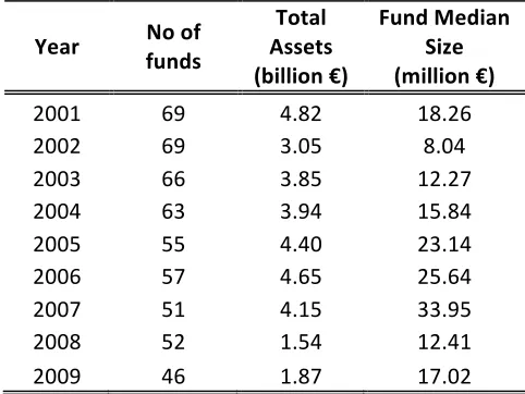
Table 1 presents some interesting figures regarding the evolution of domestic equity

fund industry such as number of funds, total assets under management and fund

[image:7.595.176.417.408.589.2]

median size.

Table 1

Evolution of domestic equity fund industry

Year No of funds

Total Assets (billion €)

Fund Median Size (million €)

2001 69 4.82 18.26 2002 69 3.05 8.04 2003 66 3.85 12.27 2004 63 3.94 15.84 2005 55 4.40 23.14 2006 57 4.65 25.64 2007 51 4.15 33.95 2008 52 1.54 12.41 2009 46 1.87 17.02

Note: This table reports domestic equity fund industry figures such as number of funds, total assets and median size. Data are reported for each year during the period January 2001-December 2009. Index funds and equity funds domiciled in Luxembourg are excluded.

3. Methodology and data description

4

(8)

3.1 Data description

Our sample includes all domestic equity mutual funds which are in operation

for at least 36 months during the period June 2001- December 2009. The number of

funds included in our analysis ranges from 36 to 69. Index funds and funds that are

not domiciled in Greece are excluded from our analysis. Net asset value (NAV) of the

domestic equity funds is employed whereas market portfolio is proxied either by the

simple General Index (ASE-GI) returns or the total return General Index (ASE-GI

Total) that is inclusive of dividends distributions5. We employ Datastream’s Greek

government bond index and the risk-free rate as proxied by the three-month

government zero-coupons. Funds’ monthly NAVs were obtained from the Association

of the Greek Institutional Investors (AGII), while the other series were obtained from

Datastream. Returns of all the employed series are calculated on a monthly basis

while the benchmark portfolios were rebalanced annually.

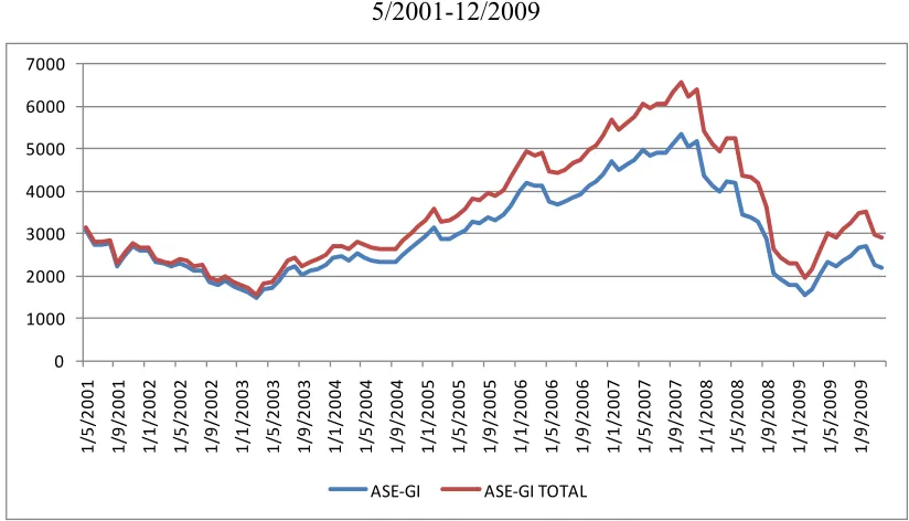
Figure 1 highlights the behavior of the employed market indices whereas in

Table 1 annual returns of both indices are displayed. Starting from late of 2003, there

is a consistent spread between the indices reflecting the effect of dividends

distributions of the stocks. It is obvious that the returns of the simple ASE General

Index can result in a substantial underestimation of the true market portfolio returns

(difference between two stock market indices ranges between 37 and 1245 units) that

could severely bias inferences of fund managers’ performance.

Figure 1

5

(9)

Evolution of ASE-GI Index and ASE-GI Total Return Index for period

5/2001-12/2009

Source: Blomberg, Datastream

Table 2

Annual returns of employed market portfolio indices

Year ASE-‐GI ASE-‐GI TOTAL

2002 -‐32.53% -‐30.20%

2003 29.46% 34.63%

2004 23.09% 27.14%

2005 31.50% 35.89%

2006 19.93% 23.13%

2007 17.86% 20.77%

2008 -‐65.50% -‐64.33%

2009 22.93% 26.37%

Source: Bloomberg, Datastream

Our strategy mimicking portfolios were constructed in the spirit of Otten and

Bams (2002) while all stocks included in the list of Worldscope for Greece were

employed. Ranking stocks with respect to the previous year’s size, we assign the top

30% by market capitalization to the big portfolio and the bottom 30% to the small

portfolio. Their return difference yields the size strategy (SMB) returns. Similarly, we

rank stocks according to last year’s returns. The difference between the top 30%

winners by market capitalization and the bottom 30% losers provides us with the

0 1000 2000 3000 4000 5000 6000 7000 1 /5 /2 0 0 1 1 /9 /2 0 0 1 1 /1 /2 0 0 2 1 /5 /2 0 0 2 1 /9 /2 0 0 2 1 /1 /2 0 0 3 1 /5 /2 0 0 3 1 /9 /2 0 0 3 1 /1 /2 0 0 4 1 /5 /2 0 0 4 1 /9 /2 0 0 4 1 /1 /2 0 0 5 1 /5 /2 0 0 5 1 /9 /2 0 0 5 1 /1 /2 0 0 6 1 /5 /2 0 0 6 1 /9 /2 0 0 6 1 /1 /2 0 0 7 1 /5 /2 0 0 7 1 /9 /2 0 0 7 1 /1 /2 0 0 8 1 /5 /2 0 0 8 1 /9 /2 0 0 8 1 /1 /2 0 0 9 1 /5 /2 0 0 9 1 /9 /2 0 0 9

[image:9.595.91.503.95.331.2]

(10)

momentum (MOM) portfolio returns. Finally, the 30% of stocks with the highest

book to-market-value ratio were assigned to the High portfolio, while the 30% of

stocks with the lowest such ratio were assigned to the Low portfolio. Their return

difference provided us with the book-to-market value (HML) strategy returns.

As already noted, managers of equity mutual funds to small and regional

markets with low trading volume for a large number of shares face another risk factor,

that is liquidity risk. We construct an additional risk factor using the daily number of

traded shares6. For each stock we calculated a daily average turnover volume and then

stocks are ranked according to this measure. We assign the bottom 10 stocks with the

lowest volume to the portfolio of illiquid stocks (low volume) and the top 10 stocks to

the portfolio of liquid stocks (high volume). Their return difference provided us with

the low minus high volume (LHVO) strategy returns. It should be mentioned that

when we construct benchmark portfolios we apply an additional filter excluding

stocks that fall in the lowest 25% percentile of total market value of the available

stocks that usually lie outside domestic fund managers’ investment universe.

3.2 An asset factor performance evaluation model

Raw returns of the funds were calculated employing the standard formula7:

(1)

In the present study we examine funds’ performance using two different measures that

adjust fund returns for exposure to known sources of investment risk. The first

measure we employ is Jensen’s alpha (1968) given by:

t f M M JENSEN f

p R R R

R − =α +β ( − )+ε (2)

6

Datastream VO data item

7

Dividends are not included in funds’ return calculation since domestic equity funds do not distribute dividends separately to their shareholders

1 1) (

− −

−

=

pt pt pt

pt

NAV NAV NAV

(11)

where Rf is the risk-free rate and RM is the stock market return

However, CAPM-rooted performance measures like Jensen’s alpha are mostly static

ignoring important aspects of managers’ investment behavior. Stated differently,

when we evaluate investment performance of actively managed funds our main

concern is to distinguish between managers that possess pure skill and those that just

bet on the price movements of certain market sectors or stocks. As Elton et al. (1996)

and Gruber (1996) suggest, we include the bond returns in our regressions in order to

capture the fund return created by bond holdings. Finally, following a series of papers

documenting the importance of stock-level liquidity for expected stock returns

(Amihud 2002, Lee 2011 etc) we incorporate a liquidity-mimicking risk factor.

Therefore, we employ the intercept from a 6-factor performance evaluation model

incorporating all known risk factors derived from:

t f

B f

M M p f

p R R R SMB HML MOM R R LHVO

R − =α +β ( − )+β1 +β2 +β3 +β4( − )+β5 +ε

(3)

where SMB (Small Minus Big) is the return generated by the size strategy,

HML (High Minus Low) is the return generated by the book-to-market value ratio

strategy

MOM (Momentum) represents the returns of the momentum strategy

RB represents the Bond Index returns and

LHVO represents the liquidity factor returns.

Since our liquidity-risk factor may be correlated to the other regressors we conducted

an orthogonalization of the liquidity-risk factor. Orthogonalization consists of

regressing the returns of the liquidity portfolio on the returns of the rest benchmark

factors such as the market returns, the SMB, HML and MOM returns, that is:

LHVO t

t t

mt p

t R SMB HML MOM

(12)

Then, the residuals of the first step regression are employed in place of the liquidity

factor returns. This adjustment helps us alleviate any potential biased inferences

resulting from multicollinearity in our regression.

3.3 Definition of variables

The various costs incurred by fund investors are used to cover the different

administrative, operating, advertising or marketing expenses. Usually, fund expenses

include the management fee, the custodian’s and auditors’ fees, stock transaction

costs and other costs that are related to research or customer support. It is worth to

note that the different types of loads (front or back-end, deferred sales) are excluded

from the calculation of the expense ratio. Total expense ratio can measure the ability

of a fund to keep its total costs at a low level, hence delivering higher net returns to its

shareholders. Consistent with the Grossman & Stiglitz (1980) hypothesis, a negative

relationship between fund performance and total expense ratio would suggest that

superior funds are more operationally efficient and can process all available

information better than the rest funds.

Fund age measures its ability to survive in a highly competitive environment,

its prestige or in other words the dedication that receives from its investors. Funds’

total assets reflect its popularity and its past growth. A positive relationship between

fund size and performance would be indicative of economies of scale. On the other

hand, there is a belief that a large fund size may have a detrimental effect on fund

performance due to trading costs associated with liquidity or price impact (Andre

Perold & Robert S. Salomon 1991, Roger Lowenstein 1997) especially in thinly

traded markets. The exploration of the relationship between performance and fund

assets would be useful for investors, particularly in light of the large inflows that

usually increase the mean fund size during bull stock markets. The fund size could

also be related to problems that may arise due to asymmetric information between the

shareholders and the fund manager. Fund managers are likely to be engaged into

moral hazard actions by expropriating wealth from investors through charging higher

(13)

depends crucially on the scale ability of fund investments (see among others Berk &

Green 2004).

The impact of cash holdings’ on fund’s performance is twofold. The portion of

fund assets that held in cash is associated with the open end structure of funds. In

order to meet investor redemptions, funds must either liquidate securities or hold cash.

Liquidating stock holdings entails transaction costs while holding cash results in

lower gross expected returns especially during rising stock markets. According to

some researchers8 cash holdings are the predominant tool for money managers to time

the market. A positive relationship between performance and cash might indicate that

managers that hold more cash to satisfy investors’ withdrawals generate larger excess

returns than those that hold less cash and liquidate securities holdings to meet

investors’ redemptions. Similarly, a positive relationship might be indicative of

market timing ability possessed by fund managers.

3.4 Determinants of fund performance under quantile regression

In order to address the sensitivity of fund performance to various operational and cost

characteristics in different quantiles of returns dispersion we employ the quantile

regression method proposed by Koenker and Bassett (1978) and Koenker (2005).

Quantile regression is a very useful and robust tool in cases that distribution of the

dependent variable departs from normality. It can provide an accurate estimate of the

relationship between the dependent and the independent variable at prespecified areas

of the distribution of the dependent variable.

In particular, quantile regression alleviates one of the fundamental constraints of the

traditional conditional-mean regression models and permits the estimation of various

quantile functions, helping to analyze the relationship between the variables in the

tails of the distribution.9 Given that the quantile analysis does not rely on any

assumption with respect to the conditional distribution of funds’ performance it is

8

Wermers (2000) reported that on average only 83% of a fund’s assets is in equity. He claimed that ‘the substantial portion of the underperformance of mutual funds versus stock indices can be traced to fund investments in non stock securities.’ His findings reveal that non stock holdings result in 70 b.p. per year lower returns.

9

Generally, each quantile regression defines a particular, centre or tail, point of a conditional distribution. This approach also allows the estimation of the median (0.₅th_{quantile) function as a}

(14)

particularly suitable in the context of our study that is plagued with significant return

dispersion. As a result the quantile analysis deviates from conditional-mean models,

as it allows for fund performance heterogeneity.

Stated differently, quantile regression is an advanced technique designed to provide a

thorough statistical analysis of the implicit variety of dependence among variables by

supplying efficient estimations of conditional quantile functions along with the

conditional mean functions.

The τ-th conditional quantile function of a distribution is defined as:

β

τ _iT

y x x

Q

i( / )= (5)

where yi is a dependent variable and xi is a vector of independent variables and β is a

vector of coefficients to be estimated. The estimator of βˆ(τ) results from the solution

of the following weighted minimization problem:

) ( min arg ) ( ˆ 1 β ρ τ β τ β T i i n i R x y p − =

∑

= ∈ (6)

where ρτ is a weighting function. For any τ∈(0,1)a weighting function takes the form:

{

₍ ₁₎ _ifif_uui ₀0 i

)

(

≥ −

=

i i u u i

u

τ τ τ

ρ

 where ui=yi-xi

T

β (7)

Combining equations (6) and (7) we get the following expression:

} ) 1 ( { min arg ) ( ˆ : 1 : 1 β β β τ β τ τ β T i T

i iy x

n i T i i x y i n i T i

i x y x

y 

∑

= ≥ = − − + −

= ₍₈₎

Observing equation (8) we conclude that the quantile regression estimator is obtained

by minimizing the weighted sum of absolute errors where the relative weights depend

on the specified quantile.

Therefore, quantile regressions for estimating funds’ performance and a set of

explanatory variables, Xt, for τ quantiles are characterized as:

τ τ

τ τ Xt =α +β Expt+β Assetst+β Aget+β Casht +ε

(15)

where

the dependent variable is funds’ abnormal return measured by augmented Carhart alpha calculated in previous section

Expt measures total expense ratio of fund i which is calculated as the ratio of funds’

total expenses to the average of total net assets during every year.

Assetst which equals fund year-end assets measured in euros.

Aget which is measured by the number of years since fund’s inception

Casht which measures the portion of fund assets that is invested in cash or cash

equivalents

In the context of the present analysis we conduct a simultaneous quantile regression

analysis, that is, we will simultaneously derive parameter estimates for various

quantile regressions namely 0.05, 0.25, 0.5, 0.75 and 0.95. It should be noted that

simultaneous quantile regression analysis is of particular importance since standard

errors are obtained by employing the bootstrap method (see Gould, 1997). Also, this

kind of analysis results in consistent and robust inferences in cases when the error

term is assumed to be heteroscedastic and non-normally distributed.

4. Empirical results

Table 3 contains descriptive statistics on the monthly return distributions of the 69

funds and benchmark portfolios for the period June 2001-December 2009. It

illustrates the first two moments (mean & standard deviation) the minimum and the

maximum of the monthly returns.

(16)

Descriptive statistics of funds and benchmark portfolios

All funds

Surviving

funds SMB HML MOM LHVO ASE-GI

ASE-GI Total Return

Mean -0.22% -0.15% -0.40% 0.60% -0.11% -0.20% -0.29% -0.03%

Median 0.76% 0.83% -0.80% 0.06% 0.88% -0.19% 0.41% 0.60%

Max. 15.98% 15.94% 20.83% 16.09% 12.73% 23.00% 21.78% 21.78%

Min. -23.47% -23.27% -12.65% -6.05% -30.10% -21.17% -28.31% -28.26% Std.

Dev. 6.50% 6.50% 5.80% 3.90% 6.20% 6% 7.70% 7.70% Note: This table presents some summary statistics for monthly raw returns of the equally weighted portfolios of domestic equity funds and for the benchmark factors computed for the period of June 2001 to December 2009. “All” includes both surviving and non-surviving funds.

4.1 Jensen’s (1968) model

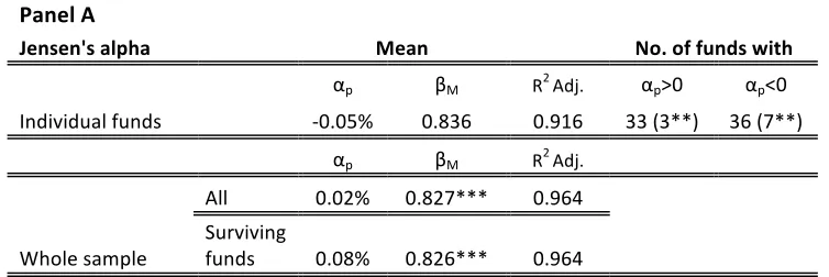
We start our analysis by examining overall performance according to the first

performance measure. Panel A of Table 4 displays average estimates of funds’

abnormal return employing ASE-GI along with the distribution of positive and

negative performance. For the overall period, average fund exhibits slightly negative

performance. In fact, the average estimate of fund performance is -0.05% while there

are only 3 funds exhibiting statistically significant positive performance at 5% level

and 7 funds statistically significant negative performance. These results are suggestive

for the absence of selectivity skills among fund managers, confirming most studies on

performance evaluation which lend support to the efficient market hypothesis.

Moreover, this finding is consistent with the absence of performance persistence

documented by Babalos et al (2008) for the domestic equity fund industry. Of course,

it should be noted that this finding does not preclude the existence of a manager

possessing significant stock picking ability.

Next, if we consider an equal weighted portfolio of all funds in our sample we

observe an almost similar performance as in the previous case whereas the portfolio

including only surviving funds exhibits a higher abnormal return. The latter might

somewhat indicative of the presence of a survivorship bias effect documented

extensively in the literature10.

10

(17)

However, as it has already been mentioned, the ASE-GI is not inclusive of the

various dividends distributions of the stocks which in turn might result in a serious

underestimation of market portfolio true return. Therefore, results of estimating

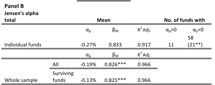
equation (3) utilizing ASE-GI Total Return in place of the simple index are presented

in Panel B of Table 4. The main finding is that there is a significant shift of fund

performance towards negative levels as it is reflected by the average estimate of alpha

(-0.27%) and the number of statistical significant negative performance (21 funds).

Underperformance is more pronounced considering abnormal return of the equal

[image:17.595.110.487.638.764.2]

weighted portfolio namely -0.19%.

Table 4

Fund performance: Jensen’s alpha

Panel A

Jensen's alpha

Mean

No. of funds with

Individual funds

αp βM R2 Adj. αp>0 αp<0

-‐0.05% 0.836 0.916 33 (3**) 36 (7**)

αp βM R2 Adj.

Whole sample

All 0.02% 0.827*** 0.964

Surviving

(18)

Panel B

Jensen's alpha total

Mean

No. of funds with

Individual funds

αp βM R2 Adj. αp>0 αp<0

-‐0.27% 0.833 0.917 11

58 (21**)

αp βM R

2

Adj.

Whole sample

All -‐0.19% 0.826*** 0.966

Surviving

funds -‐0.13% 0.825*** 0.966

Note: This table summarizes the results from the estimation of equation (3) for domestic equity funds and for the period June 2001-December 2009. Panel A of the table presents average abnormal return when market is proxied by ASE-General Index for individual funds and for the equal weighted portfolio of our funds while Panel B depicts results employing ASE-General Index Total Return respectively. All_{refers to both surviving and non-‐surviving funds during the period of analysis.}_The number of funds with positive and negative estimates of selectivity as well as the number of funds with statistically significant coefficients, adjusted for autocorrelation and heteroscedasticity according to Newey and West (1987), are also presented.

***, ** and * indicate statistical significance at the 1% , 5%) and 10% level respectively.

4.2 Estimates of asset factor performance evaluation model

Table 5 reports average equity funds’ performance and risk exposures under

the augmented Carhart model that incorporates ASE-General Total Return Index.

Average fund performance still remains negative though slightly improved compared

to the performance derived from total return Jensen model. A possible explanation

may lie in the inherent weakness of the Jensen that fails to account for the dynamic

strategies employed by fund managers. It is interesting to observe that the distribution

of funds with positive or negative performance has not changed dramatically except

for 2 funds exhibiting positive and statistical significant performance at 5%. However,

a significant difference between the two evaluation approaches lies in the explanatory

power as it is reflected in the values of adjusted R2. In particular, the asset factor

model is superior in terms of adjusted R2 with an average of 0.946 compared to 0.916

[image:18.595.111.488.72.222.2]

(19)

liquidity-augmented evaluation model outranks its single index counterpart in all of the

estimated regressions. In general, in terms of the explanatory power of evaluation

models we can also infer that the level of funds’ non-systematic risk is particularly

low for the period under analysis. With respect to the latter finding, portfolios of

domestic equity funds appear sufficiently diversified.

Asset factor evaluation models allow robust inferences when considering

stock picking ability of fund managers. Regressing a fund’s realized returns on the

returns of zero investment factor mimicking portfolios decomposes pure ability from

passive exposure to common risk factors. Therefore, examining the estimated

coefficients of funds’ returns relative to the benchmark factors we can draw

conclusions regarding fund managers’ incentives and the resulting performance. For

the purposes of our study we will focus on the exposures of the equal weighted

portfolio either including all or only the surviving funds.

Observing the coefficients of the augmented Carhart model we document a

substantial exposure of domestic equity funds’ to specific risk factors. Firstly, it is clear that domestic equity funds exhibit a highly significant exposure (0.170) to the

size factor during our period of analysis. Thus, we infer that domestic equity fund

managers show a significant tilt toward small-cap stocks. Regarding the momentum

factor we document a tendency of domestic fund managers to follow stocks that have

good track record in the pasti.e., buying stocks that were past winners and selling past

losers. Our findings are in line with US evidence such as Carhart (1997) reporting that

fund managers tend to follow momentum and small cap strategies. In light of the new

stock level liquidity factor, the preliminary results are fairly interesting. Particularly,

the coefficient of the liquidity factor is positive and statistically significant at 1%

indicating the presence of relatively illiquid stocks in funds’ portfolio holdings.

Table 5

Estimates of asset factor evaluation model

Augmented Carhart total

alpha Mean No. of funds with

Individual funds

αp βM βSMB βHML βMOM βLIQ

R2

Adj. αp>0 αp<0

(20)

αp βM βSMB βHML βMOM βLIQ

R2

Adj.

Whole sample

All -‐0.12% 0.849*** 0.170*** -‐0.036 0.074*** 0.046*** 0.986

Surviving

funds -‐0.06% 0.850*** 0.168*** -‐0.027 0.081*** 0.047*** 0.987

Note: This table summarizes the results from the estimation of equation (4) for domestic equity funds and for the whole period June 2001-December 2009. Mean monthly abnormal return when market portfolio is proxied by ASE-General Total Return Index for individual funds and for the equal weighted portfolio of the available fund is displayed. All _{refers to both surviving and non-‐surviving}

funds during the analyzed period. The distribution of funds with positive and negative estimates of selectivity as well as the number of funds with statistically significant coefficients, adjusted for autocorrelation and heteroscedasticity according to Newey and West (1987), are also presented. ***, ** and * indicate statistical significance at the 1% , 5%) and 10% level respectively.

4.3 Fund performance in sub-periods

In order to draw more robust inferences regarding managerial skills we divide

total sample period into two sub-periods of equal length. Table 6 illustrates the results

from estimating Jensen total alpha model employing monthly returns of an equal

weighted portfolio of sample funds. With respect to estimated abnormal return, we

document a highly significant fund undeperformance during the first sub-period

which during the second half turns into a neutral performance. The results also show

that most funds decrease their exposition to the market in the second sub-period

which might be related to the general negative market sentiment triggered by the

financial turmoil during 2008. In this context, we could claim that there is mild

evidence of equity funds involving into a market timing strategy shifting their

systematic risk levels.

In Table 7 we report estimates of the asset factor model for the two

sub-periods. In general, performance derived from the 6-factor model was found quite

robust among the different sub-periods. It is interesting to note that in both periods

fund performance appears statistically insignificant and close to zero. With regard to

(21)

the momentum factor was documented. Particularly, the momentum coefficient

displays a rather substantial increase from the statistically insignificant 0.032 in the

first period to the statistically significant 0.113 at 1% level in the second period. The

level of diversification of funds remained high for both sub-periods as it is revealed

[image:21.595.169.427.248.432.2]

by the high values of adjusted R2.

Table 6

Estimates of Jensen total alpha model in sub-periods

Jensen's

total alpha

Subperiod 1 αp βM R

2

Adj.

Whole sample

All -‐0.44%*** 0.852*** 0.964

Surviving

funds -‐0.35%*** 0.857*** 0.967

Subperiod 2 αp βM R2 Adj.

Whole sample

All 0.04% 0.811*** 0.969

Surviving

funds 0.07% 0.806*** 0.968

Note: This table summarizes the results from the estimation of equation (3) for the equal-weighted portfolio of domestic equity funds for two equal length sub-periods. All refers to both surviving and non-surviving funds during the analysis. Regressions have been adjusted for autocorrelation and heteroscedasticity according to Newey and West (1987) method.

Table 7

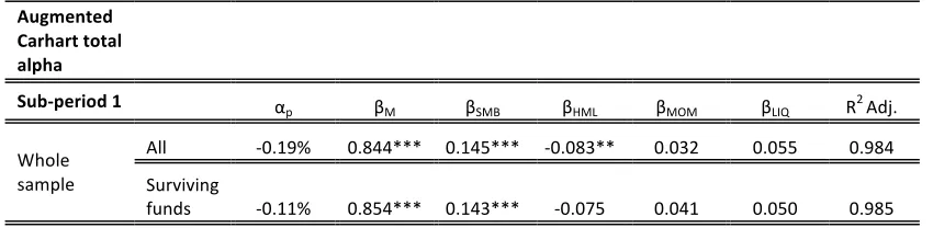
Estimates of augmented Carhart total alpha model in sub-periods

Augmented Carhart total

alpha

Sub-‐period 1 _α

p βM βSMB βHML βMOM βLIQ R 2

Adj.

Whole sample

All -‐0.19% 0.844*** 0.145*** -‐0.083** 0.032 0.055 0.984

Surviving

funds -‐0.11% 0.854*** 0.143*** -‐0.075 0.041 0.050 0.985

[image:21.595.87.512.620.724.2]

(22)

Sub-‐period 2 _α

p βM βSMB βHML βMOM βLIQ R 2

Adj.

Whole sample

All -‐0.06% 0.846*** 0.164*** 0.020 0.113*** 0.042*** 0.988

Surviving

funds -‐0.03% 0.842*** 0.163*** 0.028 0.121*** 0.044*** 0.988

Note: This table summarizes the results from the estimation of equation (4) for the equal-weighted portfolio of domestic equity funds for two equal length sub-periods. All refers to both surviving and non-surviving funds during the analysis. Regressions have been adjusted for autocorrelation and heteroscedasticity according to Newey and West (1987) method.

4.4 Performance aspects of selected funds

Additional remarks can be drawn regarding funds’ performance by examining

the behavior of the best and worst funds. Therefore, in this section we present some

interesting findings regarding performance aspects and attitude towards risk for

managers of the best and the worst funds. For the purpose of our analysis we

determine eligible funds in terms of the t-statistic values of their estimated abnormal

return derived from the asset factor evaluation model. Table 8 summarizes the results

of the estimation process including abnormal return and factor loadings for the top

and worst funds. It should be noted that regressions have been adjusted for potential

bias resulting from autocorrelation or heteroskedasticity effects using Newey-West

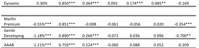
(1987) method. We can observe from Table 8 that, in the winners group two out of

three funds exhibit a substantial monthly abnormal return ranging from 0.39% to

0.55%. This means that at the fund level stock picking ability exists among domestic

equity funds especially if we take into account that the employed evaluation model

controls for the majority of naïve investment strategies. Notwithstanding, unlike what

would be expected the level of systematic risk of the funds is lower than that of the

market. A possible explanation for this fact might be related either to the selected

investment strategy exhibiting a tilt towards non-stock holdings or to fund liquidity

considerations. Regarding factor loadings in the winners group, we detect a

significant exposure of fund managers to small-cap effect and to relatively illiquid

(23)

in terms of behavioral-based investment tactics best equity fund managers appear to

follow momentum strategies.

Another key issue raised in this context is related to the conflict of interests

between shareholders and managers that has been extensively discussed in the

delegated asset management industry11. However, our results in this section highlight

a different perspective namely the alignment of interests between shareholders and

fund managers that is encountered mainly in the hedge funds’ industry. In particular,

for the first time in the traditional mutual funds’ industry, our findings suggest the

existence of an incentive effect which might play an important role in fund’s

successful track record. The term incentive effect is borrowed from hedge funds

industry and denotes a managerial performance-linked compensation. Stated

differently, in a case that a manager participates in the shareholder structure of fund’s

management company then we would expect him to share the same objectives with

fund’s shareholder that is maximization of fund return. Our argument is further

reinforced by reliable ownership data provided by domestic management companies.

Therefore, according to official data, one of the best funds in terms of risk-adjusted

return belongs to a management company whose chief executive manager is the

second largest shareholder for more than 20 years.

On the other hand, we document a significant underperformance at a micro

level among losers group. It should be noted that the magnitude of poor performance

in the losers group is comparatively higher to that of the winners’ category. It is also

interesting to observe that funds that underperform relative to passive benchmarks

exhibit high levels of systematic risk relative to the market portfolio which in turn

might indicate a false market timing strategy.

[image:23.595.89.501.677.746.2]

Table 8

Estimates of the 6-factor performance model for selected funds

Fund αp βM βSMB βHML βMOM βLIQ βBOND Marfin

Athina 0.55%** 0.792*** 0.293*** 0.003 0.050 0.069* 0.141 HSBC

Midcap 0.39%** 0.736*** 0.218*** -‐0.011 0.125** 0.120*** -‐0.180

11

(24)

Kyprou

Dynamic 0.30% 0.850*** 0.364*** 0.092 0.174*** 0.085** -‐0.169

Marfin

Premium -‐0.55%*** 0.851*** -‐0.008 -‐0.061 -‐0.056 0.020 -‐0.354*** Geniki

Developing -‐1.18%*** 0.890*** 0.266*** -‐0.071 0.036 0.096 -‐0.700**

AAAB -‐1.21%*** 0.759*** 0.224*** -‐0.060 0.088 0.052 -‐0.209

Note: This table presents estimates of abnormal return employing the 6-factor model during whole sample period for the top and worst three funds. Funds’ factor loadings for the employed risk factors are also displayed. Estimates have been adjusted for heteroskedasticity and autocorrelation using Newey-West (1987) method.

4.5 Quantile estimation of fund performance determinants

To shed more light into our analysis we report the estimates of a second stage analysis

of inferred performance relative to a series of cost and operational characteristics.

Table 9 presents coefficient estimates of fund’s performance and characteristics

equation across various quantiles.

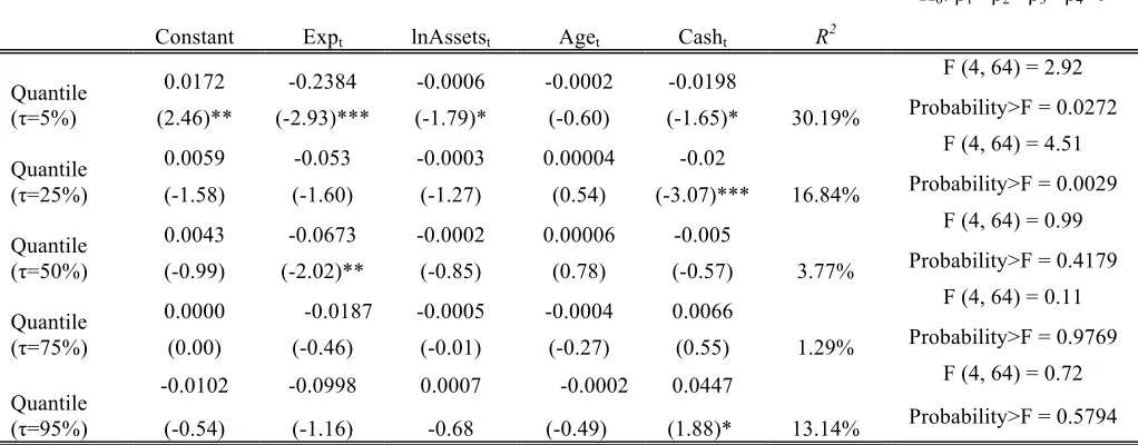
With respect to cost variable, that is total expense ratio, we document a

significant inverse relationship between fund performance and expenses in the 0.05

and 0.50 quantiles of risk-adjusted returns distributions. Stated differently, funds that

keep their expenses low achieve superior performance. The reported relationship

between performance and total expense ratio is consistent with the findings of

previous studies, we refer inter alia to Malkiel (1995), Carhart (1997), Prather et al

(2004) for US market and to Otten & Bams (2002) for 3 European markets.

Therefore, higher expenses are associated with lower risk-adjusted returns implying

the absence of economies of scale in the domestic fund industry.

Fund size seems to affect negatively performance only in low order quantile of

returns distribution (0.05). Smaller funds appear to have an advantage over larger

funds in delivering higher risk-adjusted returns. A plausible explanation for the

documented relationship between asset scale and performance would be small size

along with the illiquidity characterizing domestic capital market. Following the

[image:24.595.94.505.82.183.2]

(25)

can place all of its assets in its best ideas, an illiquid stock market forces a large fund

to invest in its less than optimal ideas and take larger positions in a stock, hence

reducing performance. Our finding is in line with the reported relationship in

Dahlquist et al (2001), Chen et al (2004), Prather et al (2004), whereas Otten & Bams

(2002), for the major European fund markets, reported significant economies of scale.

For the rest of the quantiles, fund assets exhibit a neutral effect on documented

performance.

With regard to cash variable, we reached mixed evidence, that is we observe a

significant negative effect on performance for quantiles 0.05 and 0.25. This means

that within the lowest performance groups, managers’ liquidity decisions result in an

adverse effect on fund’s final performance. In other words, fund managers for the

period under consideration lack timing ability. However, the relationship between

performance and liquid assets becomes less clear in cases of quantiles 0.50, 0.75 and

0.95 as the relationship in quantile 0.95 turns positive and statistically significant.

The finding suggests that an OLS analysis, which is close to the median quantile

(0.5), would be misleading, as it would report an insignificant coefficient for the

portion of assets held in liquid positions. On the other hand, quantile regressions by

allowing the estimation of various quantile functions of the underlying conditional

(26)

[image:26.595.42.553.189.389.2]

Table 9

Quantile estimation of fund performance determinants

Note: The table presents coefficient estimates of equation (9) employing simultaneous quantile regression. Standard errors of coefficients were obtained by bootstrapping with 100 sample replications. ***, ** and * represent statistical significance at the 1%, 5%, and 10% level, respectively.

4.5.1Quantile estimation based on size of funds

The previous section has revealed a negative effect of asset size on funds’ alpha in

low order quantiles. However, due to the special characteristics of domestic capital

market i.e. small capitalization and low trading activity, further analysis is warranted.

In addition, international evidence fails to be conclusive on the underlying

relationship12. To this end, we go a step further and examine the relationship between

fund performance and various attributes employing quantile regression analysis for

two different subsamples formed on the basis of fund size. Moreover, we form two

subgroups of funds based on the median asset size as measured by total assets. In

effect, the two subgroups are funds with low to average assets and funds with large

assets under management. Results for small funds are presented in Table 10 whereas

the estimated regressions across quantiles for larger funds are presented in Table 11.

12

Otten & Bams (2002), Chen et al (2004), Cremers et al (2011)

Constant Expt lnAssetst Aget Casht R2

H0: β1= β2= β3 =β4=0

Quantile (τ=5%)

0.0172 -0.2384 -0.0006 -0.0002 -0.0198

30.19%

F (4, 64) = 2.92

(2.46)** (-2.93)*** (-1.79)* (-0.60) (-1.65)* Probability>F = 0.0272

Quantile (τ=25%)

0.0059 -0.053 -0.0003 0.00004 -0.02

16.84%

F (4, 64) = 4.51

(-1.58) (-1.60) (-1.27) (0.54) (-3.07)*** Probability>F = 0.0029

Quantile (τ=50%)

0.0043 -0.0673 -0.0002 0.00006 -0.005

3.77%

F (4, 64) = 0.99

(-0.99) (-2.02)** (-0.85) (0.78) (-0.57) Probability>F = 0.4179

Quantile (τ=75%)

0.0000 -0.0187 -0.0005 -0.0004 0.0066

1.29%

F (4, 64) = 0.11

(0.00) (-0.46) (-0.01) (-0.27) (0.55) Probability>F = 0.9769

Quantile (τ=95%)

-0.0102 -0.0998 0.0007 -0.0002 0.0447

13.14%

F (4, 64) = 0.72

(27)

[image:27.595.118.478.200.375.2]

Table 10

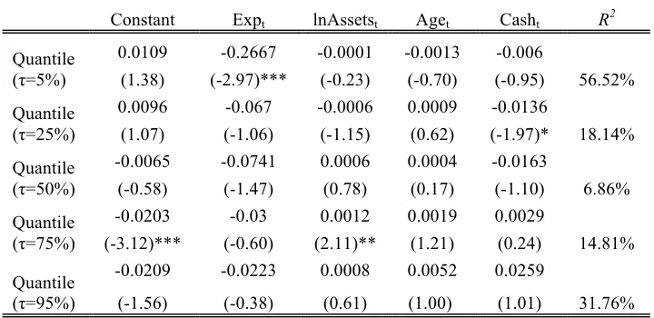
Quantile estimation of fund performance determinants of small funds

Quantile (τ=5%)

0.0109 -0.2667 -0.0001 -0.0013 -0.006

56.52% (1.38) (-2.97)*** (-0.23) (-0.70) (-0.95)

Quantile (τ=25%)

0.0096 -0.067 -0.0006 0.0009 -0.0136

18.14% (1.07) (-1.06) (-1.15) (0.62) (-1.97)*

Quantile (τ=50%)

-0.0065 -0.0741 0.0006 0.0004 -0.0163

6.86% (-0.58) (-1.47) (0.78) (0.17) (-1.10)

Quantile (τ=75%)

-0.0203 -0.03 0.0012 0.0019 0.0029

14.81% (-3.12)*** (-0.60) (2.11)** (1.21) (0.24)

Quantile (τ=95%)

-0.0209 -0.0223 0.0008 0.0052 0.0259

31.76% (-1.56) (-0.38) (0.61) (1.00) (1.01)

Note: The table presents coefficient estimates of equation (9) employing simultaneous quantile regression for small funds only. Standard errors of coefficients were obtained by bootstrapping with 100 sample replications. ***, ** and * represent statistical significance at the 1%, 5%, and 10% level, respectively.

The findings for the group of smaller funds are qualitatively similar to those

reported for the whole sample. Expenses are found to affect negatively performance

especially in low order quantile. However, contrary to the previous findings asset size

is reported to matter this time around as it carries a positive sign and it is statistically

significant in high order quantile of 0.75 insinuating a different view regarding asset

scale and fund performance for smaller funds. In the spirit of Chen et al (2004), we

claim that in light of the special characteristics of domestic capital market13 a large

asset size could be a burden for funds resulting ultimately in lower risk-adjusted

returns.

13

(28)

[image:28.595.123.475.220.396.2]

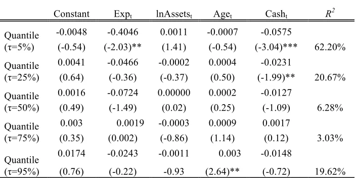
Table 11

Quantile estimation of fund performance determinants of large funds

Quantile (τ=5%)

-0.0048 -0.4046 0.0011 -0.0007 -0.0575

62.20% (-0.54) (-2.03)** (1.41) (-0.54) (-3.04)***

Quantile (τ=25%)

0.0041 -0.0466 -0.0002 0.0004 -0.0231

20.67% (0.64) (-0.36) (-0.37) (0.50) (-1.99)**

Quantile (τ=50%)

0.0016 -0.0724 0.00000 0.0002 -0.0127

6.28% (0.49) (-1.49) (0.02) (0.25) (-1.09)

Quantile (τ=75%)

0.003 0.0019 -0.0003 0.0009 0.0017

3.03% (0.35) (0.002) (-0.86) (1.14) (0.12)

Quantile (τ=95%)

0.0174 -0.0243 -0.0011 0.003 -0.0148

19.62% (0.76) (-0.22) -0.93 (2.64)** (-0.72)

Note: The table presents coefficient estimates of equation (9) employing simultaneous quantile regression for large funds only. Standard errors of coefficients were obtained by bootstrapping with 100 sample replications. ***, ** and * represent statistical significance at the 1%, 5%, and 10% level, respectively.

Regarding larger funds a finding worth noting is the importance of expenses.

As before, in low order quantiles, expenses carry a negative sign but their impact on

performance is much higher. In particular, for larger funds an increase in expenses by

1% results in lower performance by approximately 0.40% whereas for smaller funds

the reduction in performance equals 0.26%. Among the rest variables, cash appears to

affect negatively performance in low order quantiles i.e. 0.05 and 0.25. This finding

implies that managers’ fail to shift the composition of their portfolio to more

profitable investment opportunities than cash or cash equivalents but rather they

follow a more passive strategy that leads ultimately in lower performance. Finally, we

observe that for larger funds age of the fund plays an important role for fund

(29)

4.5.2 Quantile estimation based on size of funds: the impact of liquidity

Following Chen et al (2004) we investigate in detail the role of liquidity for fund

performance. To this end, we perform a simultaneous quantile regression of fund

performance characteristics including the estimated liquidity factor sensitivity

loading14 as a separate regressor:

τ τ

τ τ Xt =α +β Expt +β Assetst +β Aget +β Casht +β Liqt+ε

Q ( / ) 1 2ln 3 4 5 ₍₁₀₎

where Liqt stands for Liquidity sensitivity factor estimated from equation (4)

As in previous section, we take into account the asset size of funds and we, thus,

estimate Equation (10) for two different fund groups. Results of the quantile

regressions are presented in Tables 12 and 13 respectively.

An interesting finding that emerges from current analysis is the positive sign of

liquidity factor on fund’s performance across quantiles for small funds. In particular,

in the median quantile the effect of liquidity is found statistically significant

indicating an implicit tendency of small funds’ managers to earn abnormal returns by

exploiting liquidity related premiums. Once more, in low order quantiles, expenses

carry a negative sign and are statistically significant. However, and interestingly,

expenses affect performance negatively at 10% statistical significance in high order

quantile of 0.95 and in the median. This implies that once we take into account for

liquidity expenses gain in importance.

Table 12

Quantile estimation of fund performance determinants of small funds: the impact of liquidity

14

(30)

Constant Expt lnAssetst Aget Casht Liqt R2

Quantile (τ=5%)

0.0139 -0.3149 -0.0003 -0.0014 -0.0031 0.0214

57.76% (1.39) (-2.84)*** (-0.43) (-0.67) (-0.33) (0.84)

Quantile (τ=25%)

0.0117 -0.0795 -0.0008 0.0011 -0.0124 0.0126

21.32% (1.25) (-0.84) (-1.08) (0.46) (-1.17) (1.20)

Quantile (τ=50%)

0.0027 -0.0891 -0.00010 0.0008 -0.0029 0.0143

15.63% (0.22) (-1.91)* (-0.15) (0.35) (-0.30) (2.09)**

Quantile (τ=75%)

-0.0079 -0.0718 0.0001 0.005 0.0105 0.0125

17.42% (-0.48) (-1.13) (0.10) (1.78)* (0.58) (1.29)

Quantile (τ=95%)

-0.0169 -0.1246 0.0010 0.0047 0.0087 0.0162

40.13% (-2.36)** (-1.96)* (1.43) (1.25) (0.29) (1.40)

Note: The table presents coefficient estimates of equation (10) employing simultaneous quantile regression for large funds only. Standard errors of coefficients were obtained by bootstrapping with 100 sample replications. ***, ** and * represent statistical significance at the 1%, 5%, and 10% level, respectively.

Last, from Table 13 we infer that stock level liquidity is irrelevant for the

performance of larger funds. In addition, in low order quantiles and in the median

[image:30.595.92.494.607.763.2]

quantile expenses carry a negative sign that is highly statistically significant.

Table 13

Quantile estimation of fund performance determinants of large funds: the impact of liquidity

Constant Expt lnAssetst Aget Casht Liqt R2

Quantile (τ=5%)

-0.0072 -0.5214 0.0013 0.0000 -0.0504 0.0256

63.84% (-0.63) (-2.66)*** (1.55) (0.04) (-2.70)*** (1.61)

Quantile (τ=25%)

0.0026 -0.0501 -0.0001 0.0003 -0.0198 0.0009