Munich Personal RePEc Archive
A New Approach to Infer Changes in the
Synchronization of Business Cycle Phases
Leiva-Leon, Danilo
Bank of Canada
17 June 2013
A New Approach to Infer Changes in the Synchronization
of Business Cycle Phases
Danilo Leiva-Leony
Bank of Canada
Abstract
This paper proposes a Markov-switching framework useful to endogenously identify regimes where economies enter recessionary and expansionary phases synchronously, and regimes where economies are unsynchronized following independent business cycle phases. The reliability of the framework to track synchronization changes is corrobo-rated with Monte Carlo experiments. An application to the case of U.S. states reports substantial changes over time in the cyclical a¢liation patterns of states. Moreover, a network analysis discloses a change in the propagation pattern of aggregate contrac-tionary shocks across states, suggesting that regional economies in U.S. have become more interdependent since the early 90s.
Keywords: Business Cycles, Markov-Switching, Network Analysis.
JEL Classi…cation: E32, C32, C45.
1
Introduction
The analysis of business cycles synchronization provides crucial information for policy makers in determining the regions, in the case of a country, or the countries, in the case
of a union, more sensitive to economic policies or aggregate economic shocks. Most of the related studies have mainly focused on describing economies’ cyclical association patterns
during a given time span, however few has been done in assessing potential changes in those patterns occurred during such time span, which can be caused by a variety of reasons, such as policy changes, trade agreements, economic unions, aggregate recessionary shocks, etc.
Due to the asymmetric nature of business cycles, multivariate Markov-switching (MS) models have become a useful tool in analyzing the synchronization of countries, Smith
and Summers (2005), Camacho and Perez-Quiros (2006), among others, or the regions of a country, Owyang et al. (2005) and Hamilton and Owyang (2012). In these studies, real economic activity is modeled as a function of a latent variable which indicates, at
each time period, if the economy is in a recessionary or in an expansionary phase. These studies provide an overall picture about the synchronization between the business cycles
phases of di¤erent economies, although they are not able to endogenously identify potential synchronization changes. This is because, in order to preserve parsimony in the models, a
non-explored question that could help to unveil this feature has remained unnoticed: how does the dependency relationship between the latent variables governing a multivariate MS model vary over time?
The approaches used in the literature to deal with multivariate MS frameworks tra-ditionally assume constant dependency relationships between the latent variables, which
can be sorted into two categories. The …rst one refers to studies where such relation is just a priori assumed based on the researcher’s judgment. Multivariate MS models are usually analyzed under three di¤erent settings, Hamilton and Lin (1996) and Anas et al. (2007). The …rst one refers to the case where all series follow common regime dynamics, Krolzig (1997) and Sims and Zha (2006). Second, the use of totally independent Markov
chains, which is the most followed approach, Smith and Summers (2005) and Chauvet and Senyuz (2008). Third, the dynamics of one latent variable precedes those of other latent
variables, Hamilton and Perez-Quiros (1996) and Cakmakli et al. (2011), which allows for possibly di¤erent number of lags.1 Accordingly, the obtained regime inferences and …nal interpretations of the model’s output may substantially vary depending on the type
of judgment. There is also the case of a general Markovian speci…cation which involves
1Another type of relationship, under a univariate framework, is presented in Bai and Wang (2011) where
the full transition probability matrix, however, it brings computational di¢culties as the model increases in the number of series, states or lags, becoming also less straightforward to interpret, and moreover, it does not allow to endogenously infer the type of relationship
between the latent variables.
The second category focuses on makinga posterioriassessments of the synchronization between MS processes, providing "average" dependency relationship estimates. Works in this line are Guha and Banerji (1998) and Artis et al. (2004), which after estimating
dif-ferent univariate models, compute cross-correlations between the probabilities of being in recession as measure of synchronization. However, as shown in Camacho and Perez-Quiros (2006), these approaches may lead to misleading results since they are biased to show
relatively low values of synchronization precisely for countries that exhibit synchronized cycles. This suggests that a bivariate framework would provide a better characterization
of pairwise synchronization than two univariate models.
Regarding the analysis of pairwise business cycle contemporaneous synchronization,
Phillips (1991) point out the two extreme cases presented in the literature; the case of complete independence (two independent Markov processes are hidden in the bivariate speci…cation) and the case of perfect synchronization (only one Markov process for both
variables). In this line, Harding and Pagan (2006) propose a test for the hypotheses that cycles are either unsynchronized or perfectly synchronized, also Pesaran and
Tim-mermann (2009) focus on testing independence between discrete multicategory variables based on canonical correlations. Another similar approach followed by Camacho and Perez-Quiros (2006), Bengoechea et al. (2006), and Leiva-Leon (2014), consists on
model-ing the data generatmodel-ing process as a linear combination between the unsynchronized and perfectly synchronized cases. Despite the fact that these approaches provide inference on
the dependency relationship among the latent variables, they are not able to analyze it in a time-varying fashion.
This paper provides a new approach to infer the time-varying relationship between the latent variables governing multivariate MS models. This information allows to en-dogenously identify regimes where two economies enter recessions and expansions
synchro-nously, from regimes where the economies are unsynchronized, experimenting independent business cycle phases. In contrast to the previous related literature, the proposed …lter
not only provides a full characterization of the regime inferences, but simultaneously also provides inferences on the type of synchronicity that both economies experience at each
period of time.
The model is estimated by Gibbs sampling and its reliability is assessed with Monte Carlo experiments, …nding it a suitable approach to track changes in the synchronization
changes in the clustering and interdependence patterns that could experiment, not only two, but many economies. This is done by relying on network analysis, where economies take the interpretation of nodes and links between pairs of nodes are given by the
esti-mated synchronicity, fully characterizing a business cycle network governed by Markovian dynamics.
The proposed framework is applied to investigate potential variations in the cycli-cal interdependence between the states of U.S., obtaining three main …ndings. First, the
results report the existence of interdependence cycles which are associated to NBER reces-sions, such cycles are de…ned as periods characterized by low cyclical heterogeneity across states, experienced during the recessionary and recovery phases, followed by longer periods
of high cyclical heterogeneity, occurred during the phases of stable growth. Second, there are substantial variations in the grouping pattern of states over time, going from a scheme
characterized by several clusters of states to a core and periphery structure, composed by highly and lowly synchronized states, respectively. Third, the network analysis documents
a change in the propagation pattern of contractionary shocks across states, which consist on going from recessions characterized by shocks being spread mainly toward few but big states in GDP share terms, until the nineties, to recessions where shocks have been more
uniformly spread to all states, after that time, suggesting that U.S. economy’s regions have become more interdependent since the early 90s.
The paper is structured as follows. Section 2 presents the proposed time-varying synchronization approach, describes the …ltering algorithm and reports the Monte Carlo simulation results. Section 3 analyzes the dynamic synchronization of business cycle phases
in U.S. states, by relying on bivariate, multivariate and network analyses. Finally, Section 4 concludes.
2
The Model
Let yi;t be the growth rate of an economic activity index of economy i, which can be
modeled as a function of a latent or unobserved state variable,Si;t, which indicates if such
economy is in a recessionary or expansionary regime, an idiosyncratic component, i;t, and
a set of additional parameters, i. Accordingly, fori=a; b,
ya;t =f(Sa;t; a;t; a) (1)
yb;t=f(Sb;t; b;t; b); (2)
the goal of this section is to provide assessments on the synchronization between Sa;t and
Following the line of Owyang et al. (2005) and in Hamilton and Owyang (2012), who rely on AR(0) MS speci…cation, I consider the following tractable bivariate two-state Markov-switching speci…cation: " ya;t yb;t # = "
a;0+ a;1Sa;t
b;0+ b;1Sb;t
# + " "a;t "b;t # ; " "a;t "b;t # N " 0 0 # ; " 2 a ab ab 2b
#!
: (4)
It is worth to note that the results derived in this section can be straightforwardly extended to speci…cations including lags in the dynamics, however Camacho and Perez-Quiros (2007) show that positive autocorrelation existing in macroeconomic time series can
be better captured by shifts between business cycle states rather than by the standard view of autoregressive coe¢cients. The model can also be extended to allow for regime switching
in the variance-covariance matrix, however since the empirical application focuses on the period after the Great Moderation, such feature is not included in the model.
The state variable Sk;t indicates that ykt is in regime 0 with a mean equal to k;0 , whenSk;t= 0, or thatyktis in regime 1 with a mean equal to k;0+ k;1, whenSk;t= 1, for
k =a; b. Moreover Sa;t and Sb;t evolve according to irreducible two-state Markov chains,
whose transition probabilities are given by
Pr(Sk;t=jjSk;t 1 =i) =pk;ij, fori; j= 0;1and k=a; b: (5)
To characterize the dynamics of yt = [ya;t; yb;t]0, the information contained in Sa;t
and Sb;t can be summarized in the state variable, Sab;t, which accounts for the possible combinations that the vector, Sab;t = a;0+ a;1Sa;t; b;0+ b;1Sb;t 0, could take trough
the di¤erent regimes.
Sab;t=
8 > > > > > < > > > > > :
1, IfSa;t= 0; Sb;t= 0
2, IfSa;t= 0; Sb;t= 1
3, IfSa;t= 1; Sb;t= 0 4, IfSa;t= 1; Sb;t= 1
: (6)
Following the line of Harding and Pagan (2006), the objective of the propose model is to di¤erentiate regimes where the phases of ya;t and yb;t are unsynchronized, implying
that Sa;t and Sb;t follow independent dynamics, that is
Pr(Sa;t=ja; Sb;t=jb) = Pr(Sa;t=ja) Pr(Sb;t=jb); (7)
from regimes where the phases of ya;t andyb;tare fully synchronized, entering expansions
and recessions synchronously, implying that Sa;t=Sb;t=St, that is
In order to do so, I introduce into the framework another latent variable,Vt, that takes
the value of 1 if business cycle phases are in a synchronized regime, and the value of 0 if they are under an unsynchronized regime at time t, that is
Vt=
(
0 If Sa;t and Sb;t are unsynchronized
1 If Sa;t and Sb;t are synchronized
: (9)
The latent variable Vt also evolves according to an irreducible two-state Markov chain
whose transition probabilities are given by
Pr(Vt=jvjVt 1 =iv) =pv;kl, foriv; jv = 0;1. (10)
The advantage of introducing, Vt, rather than analyzing the general Markovian
speci…-cation with the full transition probability matrix, as in Sims et al. (2008), is that all the information about the dependency relationship between the latent variables remains
summarized in a single variable, Vt, providing an easy to interpret way of assessing sync changes and being able even to provide information of the expected duration of regimes
were economies are synchronized or unsynchronized based on its associated transition probabilities. Notice that the analysis in this paper focuses on dependency, not on
cor-relations, since the objective is to determine if two economies are either synchronized or unsynchronized.
Accordingly, there is an enlargement of the set of regimes in Equation (6) which remains
fully characterized by the latent variable Sab;t, that simultaneously collects information regarding to joint dynamics, individual dynamics and their dependency relationship over
time,
Sab;t=
8 > > > > > > > > > > > > > > > < > > > > > > > > > > > > > > > :
1, IfSa;t= 0; Sb;t= 0; Vt= 0 2, IfSa;t= 0; Sb;t= 1; Vt= 0
3, IfSa;t= 1; Sb;t= 0; Vt= 0
4, IfSa;t= 1; Sb;t= 1; Vt= 0
5, IfSa;t= 0; Sb;t= 0; Vt= 1
6, IfSa;t= 0; Sb;t= 1; Vt= 1 7, IfSa;t= 1; Sb;t= 0; Vt= 1
8, IfSa;t= 1; Sb;t= 1; Vt= 1
; (11)
Inferences on the latent variableSab;t, can be computed by conditioning on Vt,2
Pr(Sab;t = jab) = Pr(Sa;t=ja; Sb;t=jb; Vt=jv)
= Pr(Sa;t =ja; Sb;t=jbjVt=jv) Pr(Vt=jv) (12)
where Pr(Sa;t = ja; Sb;t = jbjVt = jv) indicates the inferences on the dynamics of Sab;t
conditional on total independence, if Vt= 0, or conditional on full dependence, ifVt= 1.
In the former case the joint probability of Sab;t is given by
Pr(Sa;t = ja; Sb;t=jb; Vt= 0) = Pr(Sa;t=ja; Sb;t=jbjVt= 0) Pr(Vt= 0)
= Pr(Sa;t=ja) Pr(Sb;t=jb) Pr(Vt= 0); (13)
while in the latter case it is
Pr(Sa;t = ja; Sb;t=jb; Vt= 1) = Pr(Sa;t=ja; Sb;t=jbjVt= 1) Pr(Vt= 1)
= Pr(St=j) Pr(Vt= 1): (14)
Therefore, inferences on the state variable Sab;t, in Equation (6), after accounting for
synchronization, can be easily recovered by integrating Pr(Sa;t = ja; Sb;t = jb; Vt = jv)
through Vt, remaining as
Pr(Sa;t = ja; Sb;t=jb) = Pr(Vt= 1) Pr(St=j) +
(1 Pr(Vt = 1)) Pr(Sa;t=ja) Pr(Sb;t=jb); (15)
which implies that the joint dynamics of Sa;t and Sb;tremain characterized by a weighted average between the extreme dependent and independent cases, where the weights assigned
to each of them are endogenously determined by
Pr(Vt= 1) = abt : (16)
Therefore, the term abt from now on will be referred as the dynamic synchronicity
between Sa;t and Sb;t.
2.1 Filtering Algorithm
This section develops an extension of the Hamilton’s (1994) algorithm to estimate the model described in Equations (4) and (15). The algorithm is composed by two uni…ed
steps, in the …rst one the goal is the computation of the likelihoods, while in the second one, to compute the prediction and updating probabilities.
STEP 1: The parameters of the model are assumed to be known for the moment and collected in the vector
the model’s dynamics, Sab;t, can be expressed as a function of its components,
f(yt; Sab;t=jabj t 1; ) =f(yt; Sa;t=ja; Sb;t=jb; Vt=jvj t 1; ); (18)
which is the product of the density conditional on the realization of the set of regimes
times the probability of occurrence of such realizations,
f(yt; Sa;t = ja; Sb;t=jb; Vt=jvj t 1; ) =f(ytjSa;t=ja; Sb;t=jb; Vt=jv; t 1; )
Pr(Sa;t = ja; Sb;t=jb; Vt=jvj t 1; ): (19)
The trivariate probability of Sa;t = ja, Sb;t =jb and Vt =jv is obtained by using
condi-tional probabilities,
Pr(Sa;t = ja; Sb;t=jb; Vt=jvj t 1; ) = Pr(Sa;t=ja; Sb;t=jbjVt=jv; t 1; )
Pr(Vt = jvj t 1; ); (20)
where the term Pr(Sa;t = ja; Sb;t = jbjVt = jv; t 1; ) is fully characterized with the results derived in Equations (13) - (14). Thus, Equation (20) remains a function of just
Pr(Sk;t =jkj t 1; ) fork=a; b,Pr(Vt=jvj t 1; )and Pr(St =jj t 1; ). The steady state or ergodic probabilities can be used as starting values to initialize the …lter.
In order to make inferences on the evolution of single state variables, the marginal densities are obtained as
f(yt; Sa;t = jaj t 1; ) =
1 X
jb=0 1 X
jv=0
f(yt; Sa;t=ja; Sb;t=jb; Vt=jvj t 1; ); (21)
f(yt; Sb;t = jbj t 1; ) = 1 X
ja=0 1 X
jv=0
f(yt; Sa;t=ja; Sb;t=jb; Vt=jvj t 1; ); (22)
f(yt; Vt = jvj t 1; ) = 1 X
ja=0 1 X
jb=0
f(yt; Sa;t=ja; Sb;t=jb; Vt=jvj t 1; ); (23)
The marginal density associated the state variableSt requires a special treatment. When
it is assumed that the model’s dynamics are governed by only one state variables, i.e.
Sa;t =Sb;t=St, the density in Equation (18) collapses to fy(yt; St=jj t 1; ), where
fy(yt; St = 0j t 1; ) =f(yt; Sa;t = 0; Sb;t= 0; Vt= 1j t 1; ) (24)
Accordingly, the density of yt conditional on the past observables is given by
f(ytj t 1; ) = 1 X
ja=0 1 X
jb=0 1 X
jv=0
f(yt; Sa;t=ja; Sb;t=jb; Vt=jvj t 1; ); (26)
and under the assumption that Sa;t=Sb;t=St, it is given by
fy(ytj t 1; ) =
1 X
j=0
fy(yt; St=jj t 1; ) (27)
STEP 2: Onceytis observed at the end of timet, the prediction probabilitiesPr(Sk;t =
jkj t 1; )fork=a; b,Pr(Vt=jvj t 1; ) andPr(St=jj t 1; )can be updated
Pr(Sa;t = jaj t; ) = f(yt; Sa;t=jaj t 1; )
f(ytj t 1; )
(28)
Pr(Sb;t = jbj t; ) =
f(yt; Sb;t=jbj t 1; ) f(ytj t 1; )
(29)
Pr(Vt = lj t; ) =
f(yt; Vt=lj t 1; )
f(ytj t 1; ) (30)
Pr(St = jj t; ) =
fy(yt; St=jj t 1; ) fy(y
tj t 1; )
: (31)
Forecasts of the updated probabilities in Equations (28)-(31) are done by using the corre-sponding transition probabilities pa;ij; pb;ij; pij; pv;ij, in the vector , for Sa;t; Sb;t; St; Vt,
respectively.
Pr(Sk;t+1 = jkj t; ) =
1 X
ik=0
Pr(Sk;t+1=jk; Sk;t=ikj t; )
=
1 X
ik=0
Pr(Sk;t+1 =jkjSk;t =ik) Pr(Sk;t =ikj t; ); fork=a; b: (32)
Pr(Vt+1 = jvj t; ) =
1 X
i=0
Pr(Vt+1=jv; Vt=ivj t; )
=
1 X
i=0
Pr(Vt+1=jvjVt=iv) Pr(Vt=ivj t; ) (33)
Pr(St+1 = jj t; ) =
1 X
i=0
Pr(St+1=j; St=ij t; )
=
1 X
i=0
Pr(St+1 =jjSt=i) Pr(St=ij t; ). (34)
realiza-tions of Sab;t+1, relying on Equation (20)
Pr(Sa;t+1 = ja; Sb;t+1=jb; Vt+1 =jvj t; ) = Pr(Sa;t+1 =ja; Sb;t+1 =jbjVt+1=jv; t; )
Pr(Vt+1 = jvj t; ); (35)
where Equation (35) remains a function of Pr(Sk;t+1 =jkj t; ) for k = a; b, Pr(Vt+1 =
jvj t; )and Pr(St+1 =jj t; ).
By iterating these two steps for t = 1;2; : : : ; T, the algorithm provides simultaneous inferences on Sa;t,Sb;t and their dynamic synchronicity abt , de…ned in Equation (16).
Regarding the estimation of the parameters, notice that as the number of possible states increase, the likelihood function could be characterized by several local maxima causing
strong convergence problems in performing maximum likelihood estimation, Boldin (1996). Hence, given the high number of combinations of states through which the likelihood is conditioned in Equation (26), the set of parameters along with the inferences on the state
variables are estimated by using Bayesian methods. Speci…cally, I use a multivariate ver-sion of the approach in Kim and Nelson (1999), which applies Gibbs sampling procedures.
The estimation method is explained in detail in the Appendix.
2.2 Simulation Study
In order to validate the reliability of the proposed approach to assess changes in the synchronization of business cycle phases, I rely on the use of Monte Carlo experiments.
Each simulation consists of two steps. First, the generation of two stochastic processes subject to regime switching that experiment one or more sync changes. Second, by letting the econometrician just observe the generated data, but not the data generating process,
the proposed …lter in Section 2.1 along with the Gibbs sampler are applied to obtain estimates of the model’s parameters, probabilities of recession for each economy, and more
importantly the inferences on synchronization changes. Then it is addressed how well the parameter estimates and inferences match the real ones.3
Given a sample of size T, the data generating process consists on generating a …rst order Markovian process, Sa;t, with transition probability matrix
Pa = pa;00 1 pa;11
1 pa;00 pa;11 !
(36)
and an error term, eIa;t, drawn from a N(0;1). Then, given a vector of means[ a;0; a;1]0
3It is important to notice that the …lter’s performance is assessed by simulations, under the assumption
and standard error a, I generate a process yIa;t as follows
ya;tI = a;0+ a;1Sa;t+ aeIa;t; (37)
and given a vector of means[ b;0; b;1]0, standard error
b and transition probabilitiespb;00 and pb;11, the same procedure is repeated to independently generate
yIb;t= b;0+ b;1Sb;t+ beIb;t; (38)
where Sb;t is a …rst order Markovian process and eIb;t is drawn from a N(0;1). Next,
another Markovian process,St, is generated by using the transition matrix
Pab= p00 1 p11
1 p00 p11
!
; (39)
and an error term vector [eDa;t; eDb;t]0 is drawn from a bivariate normal distribution. Then, given the two vectors of means [ a;0; a;1]0 , [ b;0; b;1]0, standard errors a, b, and a parameter ab, I generate
" ya;tD
yb;tD #
=
"
a;0+ a;1St
b;0+ b;1St
#
+
"
a ab
ab b
# " eDa;t
eDb;t #
(40)
The information generated so far can be collected in two vectors, one in which two
stochastic processes are driven by two Markov-switching variables independent from each other, yIt = [ya;tI ; yIb;t]0, and the other where two stochastic processes are governed by only one Markov-switching dynamics, ytD = [yDa;t; yDb;t]0.
The premise in this paper claims that during some regimes, the output growth of two economies can follow dynamics similar to those in ytD, while during other regimes, things
can change in one, or both, of the economies, leading their joint dynamics to behave as the ones in ytI, following independent patterns. To mimic this situation, I start analyzing
the simplest case in which there is just one sync change in a sample of size T, occurred at time , with 1< < T.4 Then, letyt= [ya;t; yb;t]0 be the observed output growth of two
economies, which come from the following unobserved data generating process:
yt=
(
yDt , fort= 1; : : : ;
ytI, fort= + 1; : : : ; T ; (41)
4The selection of , is based on a random draw u, generated from a uniform distribution U[0;1], i.e.
that can be alternatively expressed as
yt=ytDVt+ (1 Vt)ytI; (42)
where Vt is an indicator variable of synchronization, which dynamics are described by
fVtgT1 =
"
1
0T
#
; (43)
with 1 being a vector of ones of size and 0T a zero vector of size T . The case
of one sync change can be easily extended to mimic the case of Z sync changes, occurred at 1; 2; : : : ; Z, with 1< 1 < 2 < : : : < Z < T, just by appropriately modifying the
dynamics in fVtgT1.
Since the data generating process and parameters are unknown by the econometrician, the Gibbs sampler is used to estimate the model’s parameters, the probabilities of recession
for each economy, and more importantly inferences on the dynamics ofVt, by relying on the …ltering algorithm proposed in Section 2.1. The criterion used to assess the performance
of the regime inferences and the synchronization is the Quadratic Probability Score (QPS) de…ned as
QP S( ) = 1
T
T
X
t=1
( Pr( = 1j T))2; for =Sa;t; Sb;t; Vt: (44)
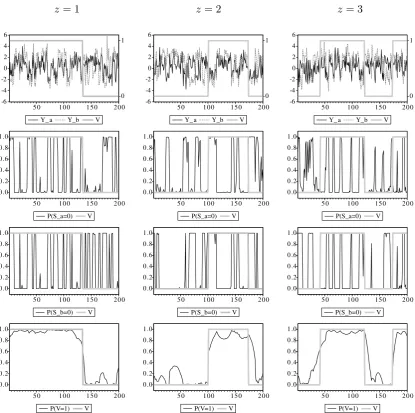
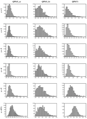
To illustrate the …ltering and estimation strategy’s performance, Figure 1 plots one
simulation for the cases in which there is one, two and three sync changes in a sample of 200 periods, i.e. for z = 1;2;3, with T = 200. For each case, the top charts plot the
two observed time series, ya;t and yb;t, generated with the parameter values in Table 1
and by using Equation (42), along with the unobserved dynamics of Vt. Both time series
show strong coherence in phases when Vt= 1, and the opposite occurs whileVt= 0. The
two middle charts plot the probabilities of recession associated to each time series, i.e.
Pr(Sk;t = 0j T), for k = a; b, showing values near to one when the corresponding time
series reports consecutive negative values, also the dynamics of Vt is plotted as reference. Finally, the bottom charts plot the computed inferences on the synchronization changes,
i.e. Pr(Vt = 1), along with the true dynamics of Vt, showing their close relation in all
the three cases and giving insights about the satisfactory performance of the proposed framework in assessing synchronization changes.
This experiment is replicated M = 1000 times for Z = 6 di¤erent cases. Each case corresponds toz changes in sync, forz= 1;2;3;4;5, and the last case considers a random
number of sync changes, i.e. unlike prede…ning the dynamics of Vtas in Equation (43), it
z=f(Vt).5
The result of the Monte Carlo simulations are reported in Table 2, showing the average over the M replications of each estimated parameter
z=
1
M
M
X
m=1 (m)
z ; (45)
where z(m) corresponds to the vector of parameters, as de…ned in Equation (17),
associ-ated to the m-th replica and thez-th case. All parameter estimates appear to be unbiased for the di¤erent values of z. Although, two features deserve attention. First, the
stochas-tic process with the highest di¤erence of the within-regime means, in this case yb;t, shows more accurate estimates, meaning that higher di¤erences provide a better identi…cation of the phases of the business cycles.6 Second, the accuracy in the estimation of the transition
probabilities decreases whenz=f(Vt), this is due to the high number of sync changes and the short duration of each change generated by letting Vt to follow Markovian dynamics.
Regarding the performance about the regime inferences, Table 3 reports the averages over theM replications of the QPS associated to the state variablesSa;t; Sb;tandVt, which
can be interpreted as the average over the M replications of the squared deviation from
the generated business cycles.
QP S( )z =
1
M
M
X
m=1
QP S( )(zm); for =Sa;t; Sb;t; Vt (46)
where QP S( )(zm), as de…ned in Equation (44), corresponds to the m-th replica and the
z-th case. The results indicate that, although inferences on the state variables in general
present high precession, the ones associated to the time series with highest di¤erence of the within-regime means, yb;t, are the most accurate. The main message of the table is
that precision of the inferences decreases as the number of sync changes,k, increases. This
feature can also be observed by looking at the histograms of the M replications plotted in Figure 2, in particular the ones associated to QP S(Vt). However, it is natural to think
on synchronization changes as events that do not occur as often as the business cycle phases of an economy, but that require longer periods of time to take place, since they
are originated from changes in the structural relationships among economies, letting the proposed model be suitable to accurately infer sync changes of business cycle phases.
5This is done using the corresponding values given in Table 1. 6The parameters associated to the variance-covariance matrix of y
t are not analyzed in Table 2 due
3
Monitoring U.S. States Business Cycles Synchronization
The last global …nancial crisis has stimulated the interest in the study of the sources
and propagation of contractionary episodes, calling to take a more careful look at the disaggregation of the business cycle in order to assess the mechanisms underlying economic ‡uctuations. On the one hand, recent work by Acemoglu et al. (2012) that relies on
network analysis, …nds that sectoral interconnections capture the possibility of “cascade e¤ects” whereby productivity shocks to a sector propagate not only to its immediate
downstream customers, but also to the rest of the economy.
On the other hand, two recent works have shown interesting features of economic
activ-ity phases synchronization when the business cycle is disaggregated at the regional level. In the …rst one, Owyang et al. (2005) investigate the evolution of the individual business cycle phases of the U.S. states. By following a univariate approach, the authors …nd that
U.S. states di¤er signi…cantly in the timing of switches between regimes of expansions and recessions, and also di¤er in the extent to which state business cycle phases are in concord
with those of the national economy. In the second one, Hamilton and Owyang (2012) use a uni…ed framework to go through the propagation of regional recessions in U.S., using a
multivariate approach that focuses on clustering the states sharing similar business cycle characteristics, …nding that di¤erences across states appear to be a matter of timing and that they can be grouped into three clusters, with some of them entering recession or
recovering before others. Although these previous studies provide useful insights about the overall synchronization pattern in given sample period, they are not able to detect
changes in such patterns occurred during such time span.
The present application intends to unify both concepts, dynamic synchronization of pairwise cycles, by using the framework proposed in Section 2, and the dynamic
interde-pendence between all U.S. states, by relying on network analysis, in order to assess the presence and the nature of potential changes in the regional propagation of contractionary
shocks. For this purpose I use data on U.S. states coincident indexes, proposed in Crone (2002) and provided by the Federal Reserve Bank of Philadelphia, as monthly indicators
of the overall economic activity at the state level for the time span 1979:08 - 2013:03, Alaska and Hawaii are excluded as in Hamilton and Owyang (2012). The Chicago Fed National Activity Index (CFNAI) is used as monthly measure of the U.S. national business
cycle. All these indexes of real economic activity, for each states and for U.S., have been constructed by the corresponding authors based on the principle of comovement among
3.1 Bivariate Analysis
The analysis for 48 U.S. states plus U.S. as a whole requires to model each of the
C249 = 1176 pairwise comparisons. To assess the performance of the proposed
Markov-switching synchronization model, two selected examples are analyzed in detail.7 The …rst
example focuses on the case of two states that present high share of national GDP, New York with 7.68% and Texas with 7.95%. Table 4 reports the Bayesian estimates for the
New York vs. Texas model, showing negative growth rates when St = 0 and positive
growth when St= 1, for both states. It is worth to highlight the estimates of the
transi-tion probabilities associated to the state variable that measures synchronizatransi-tion, Vt. The
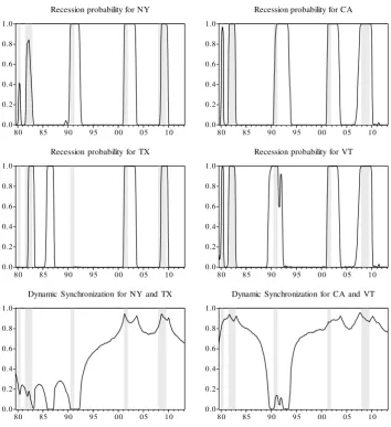
probability of remaining in a regime of high synchronization is almost equal to the proba-bility of remaining in a low sync regime, about 0.96. This result is corroborated in Chart
A of Figure 3, which plots the probabilities of recession for New York and Texas along with the corresponding time-varying synchronization, N Y;T Xt , as de…ned in Equation (16). As
can be in the top and middle charts, since the eighties until the mid-nineties these states were experimenting recessions with di¤erent timing, this is re‡ected in the low values of the synchronicity, plotted at the bottom of chart A. However, after the mid-nineties until
the present time, both economies have been experiencing the same recession’s chronology, which is consistent with the increase in the synchronicity observed after the mid-nineties.
The second example analyzes the case of two states with di¤erent GDP shares, the state with the highest one, California with 13.34%, and the state with the lowest one,
Vermont with 0.18%. Table 5 presents the Bayesian parameter estimates of the model. Unlike to the previous example, in the California vs. Vermont model, the probability of remaining in a high sync regime, 0.97, is higher than the probability of remaining in
a low sync regime, 0.93. This agrees with Chart B of Figure 3, which shows that in general both states have been experiencing the same business cycle chronology, entering
recessions and expansions synchronously, with the exception of some period. In 1989 Vermont entered in a recessionary phase, while California was still growing, until the
mid-1990, when it started to experience a recession. However, at the beginning of 1992, Vermont started an expansionary phase, while California continued in recession until 1994. These desynchronicities are re‡ected in the downturn of the time-varying sync, CA;V Tt ,
during that period, shown at the bottom panel of Chart B.
All the remaining pairwise cases were also estimated, although the results are not shown
to save space, they are available upon request to the author. Considerable heterogeneity was found in the dynamics of the estimated time-varying synchronizations, …nding cases involving signi…cant changes, and cases were the synchronization was almost constant,
makers are interested in the "big picture" of the overall regional synchronization path, other ways of summarize the information are needed.
3.2 Multivariate Analysis
As suggested by Timm (2002) and Camacho et al. (2006), multidimensional scaling (MDS)
method is a helpful tool to identify cyclical a¢liations between economies, since it seeks to …nd a low dimensional coordinate system to represent n-dimensional objects and create a map of lower dimension (k). Traditionally, studies use as input for this method a symmetric
matrix, , that summarizes the cyclical distances between economies for a given time span, each entry ij of the matrix assigns a value characterizing the distance between economies
i and j. The output of the MDS consists on one map showing the general picture for all
the cyclical a¢liations.
The dynamic synchronization measures obtained in the bivariate analysis,0 ijt 1,
can be easily converted into desynchronization measures, ijt = 1 ijt . Accordingly, ijt can be interpreted as cyclical distances allowing the construction of the dissimilarity matrix
, for each time period
t= 0 B B B B B B B B @
1 12t 13t : : : 1tn
21
t 1 23t : : : 2tn
31
t 32t 1 : : : 3tn
..
. ... ... . .. ...
n1
t nt2 nt3 : : : 1
1 C C C C C C C C A ; (47)
providing the possibility of assessing changes in the general picture of all cyclical a¢liations
of U.S. states.
In a recent work on MDS, Xu et al. (2012) proposed a way to deal with MDS in a
dynamic fashion, where the dimensional coordinates of the projection of any two objects,
i andj, are computed by minimizing the stress function
min~ij t = n P i=1 n P j=1
( ijt ~ijt )2
P
i;i( ij t )2
+
n
X
i=1
~itjt 1; (48)
where
~ijt = (jjzi;t zj;tjj2)1=2 (49)
~itjt 1 = (jjzi;t zi;t 1jj2)1=2; (50)
and at t+ 1, keeping always the same dynamics independently on its value. In principle it can be simply set up to 1, however since the data in t belong to the unit interval, for
a more adequate visual perception of the transitions between frames it is set up to 0:1.
The output of the minimization in Equation (48) provides a bidimensional representation of t.
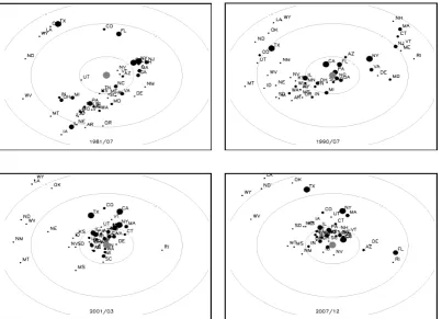
The synchronization maps of U.S. states for the …rst month of the last four recessions are plotted in the charts of Figure 4. Each point in the charts represents a states, the
mid-dle point refers to U.S. nation as a whole. The closeness between two points in the plane makes reference to their synchronicity degree, i.e. the closer are the points, the higher is their synchronization. The …gure corroborates the premise in the introduction of this
paper about the existence of signi…cant changes in the grouping pattern among regional economies through time. Speci…cally, the top-left chart plots the scenario for the 1981’s
recession, where a big group of states were in synchronized with each other, while the remaining states, such as Florida, Colorado, Texas, North Dakota, West Virginia, among
others, were following independent patterns. Also, notice that states such as Nevada, North Carolina, Vermont, Tennessee, were the ones more in sync with the U.S. business cycle during that month. The top-right corner presents the situation for the 1990’s
reces-sion, showing a di¤erent grouping pattern characterized by one big group of states in sync with each other and two small clusters, the …rst one composed by New Hampshire,
Massa-chusetts, Connecticut, Vermont, New Jersey, Maine and Rhode Island, and the second one by New York, Virginia, Delaware and Maryland. Notice that in this month, states such as Florida, Pennsylvania, California, among others, were the ones more in sync with the
U.S. cycle. The bottom charts present the scenarios for the 2001’s and 2007’s recessions, in the left and right corner respectively. Again, the pattern changed with respect to the
previous episodes, since the last two recessions were characterized by a core (composed by states highly in sync) and periphery (composed by independent states) structure, …nding
the core of the later one tighter than the in the former. The full animated representation can be found at the author’s web page.8
An additional advantage of the proposed framework is the possibility of recovering the
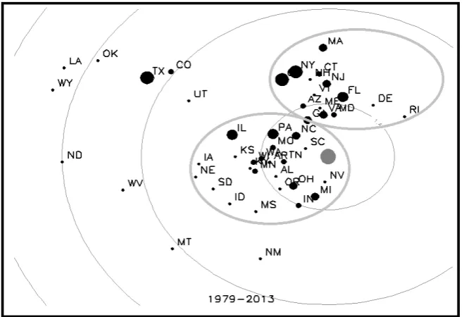
stationary measures of synchronization, by using the ergodic probabilities associated to the latent variable Vt. Chart A of Figure 5 plots the stationary grouping pattern, which
can be interpreted as the average pattern during 1979:08 - 2013:03, showing three groups of states, one of them is closer to the U.S. cycle, the second one is less but still close to
the U.S. cycle, while the third one is characterized by the states following independent dynamics. To assess if this result reconciles the one in Hamilton and Owyang (2012), Chart B of Figure 5 plots the clusters obtained by those authors, clearly …nding that both
to each cluster. Moreover, this result is not only robust to the methodology employed, but also to the data used, since Hamilton and Owyang (2012) used annualized quarter-to-quarter growth rates of payroll employment, while I use monthly growth rates of state
coincident indexes of economic activity. These facts show one of the main contributions of the proposed framework, which is provide synchronization measures that may change over
time, and moreover can be collapsed into ergodic measures that yield results consistent with the ones in previous work.
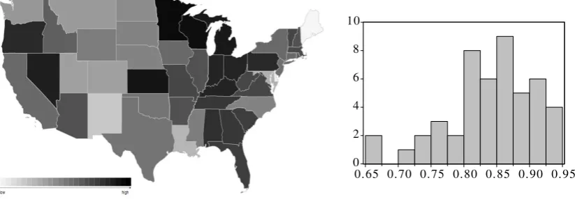
Regarding the cyclical relationship between states and the national business cycle, Table 6 reports the corresponding ergodic synchronizations, showing that it ranges from the highest, which is North Carolina with 0.91, until the lowest one, which corresponds to
Oklahoma with 0.19, revealing that states with the highest GDP share do not necessarily represent the states showing the highest synchronicity with the national business cycle.
To provide a visual perspective, Chart A of Figure 6 plots a U.S. map with the estimates obtained in this paper and Chart B, of the same …gure, plots the concordance pattern
obtained in Owyang et al. (2005) by calculating the percentage of the time two economies were in the same regime based on univariate MS models for each state. Although both results report high values in most of the states located in the east region and medium values
in few states located in the west, the stationary sync measure presents higher dispersion than the concordance, as can be seen in the associated histograms, helping to disentangle
in a more precise way the cyclical relationship between states and the nation.
3.3 Network Analysis
In recent works by Carvalho (2008), Gabaix (2011), Acemoglu et al. (2012), among others, it is shown how idiosyncratic shocks, at the …rm or sectoral level, may originate
macro-economic ‡uctuations given their interlinkages by relying on network analysis. Although, such analysis primarily relies on the economy’s sectoral disaggregation, it turns out inter-esting to assess if another type of disaggregation, e.g. regional, may also have signi…cant
implications on aggregate ‡uctuations.
The intuition behind the synchronization measure in Equation (16) relies on the fact
that if ijt is close to 1, it is likely that at time t, economies i and j are sharing the same business cycle phases, creating a link of interdependence between them. On the other hand, if ijt is close to 0, it means that they are following independent phases and
hence are not linked.9 Therefore, by lettingH =fhign1 be the set of neconomies taking the interpretation of nodes, hi for i = 1; : : : ; n, and de…ning ijt as the probability that
nodes hi and hj are linked at time t, the matrix t = 1n t, can be interpreted as
9Notice that the proposed synchronization modeling approach distinguishes between the state in which
a weighted network of synchronization with Markovian dynamics.10 Consequently, the cyclical interdependence of a large set of economies can be dynamically assessed under a uni…ed framework by relying on network analysis. It is worth to notice that although
the construction of t requires the computation several bivariate models of the type in
Equation (4), it may be less restrictive and involve less parameter and regime’s uncertainty
than the computation of a framework with similar nonlinear nature but involving all n economies simultaneously, however further research in this respect would be desired.
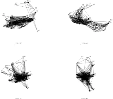
To provide a glimpse of the shape that the Markov-switching synchronization network (MSYN) have taken during contractionary episodes, the charts of Figure 7 plot the cor-responding network graph for the …rst month of the last four recessions. Given that the
MSYN is a weighted network, in order to make possible the graphical representation, a link between nodes i and j is plotted if ijt > 0:5, otherwise no link is plotted between
them. The …gure corroborates the grouping pattern of one big cluster and independent states in the 1981’s recession, some small clusters in the 1990’s recession and a core and
periphery structure and the 2001’s and 2007’s recessions, with a more concentrated core in the last recession.11
The main advantage of providing a network analysis for the present framework is
that all the information on synchronicities so far studied can be summarized in just one measure, the closeness centrality. There are several measures regarding the centrality of a
network, but given that desynchronization measures are interpreted as distances, the most appropriate one for this context is the closeness.
Two variations of the closeness centrality are analyzed in this section for robustness
purposes. For each of them, it is necessary …rst to compute the centrality of each node
Ct(i) = P 1
j6=ijtdt(i; j)
; fori= 1;2; :::; n, (51)
where d(i; j) is the length of the shortest path between nodes i and j, which can be computed by the Dijkstra’s (1959) algorithm.12 Thus, the more central is a node, the
lower is its total distance to all other nodes. Closeness can be regarded as a measure of how fast it will take to spread information, e.g. risk, economic shocks, etc., from nodeito
all other nodes sequentially. For an overview regarding to de…nitions in network analysis, see Goyal (2007).
Once the dynamic centrality of each node has been computed, the information about
1 0The term
1nrepresents a squared matrix of sizenwith all entries equal to1.
1 1Notice that although the U.S. business cycle is not included in the network analysis, just the ones of
the states, each chart in the …gure shows a close relation with the corresponding one in Figure 4
1 2For example, in a setH0=fa; b; cgwhere the distances = 1 , are given by ab= 0:5, ac = 0:9
and bc = 0:2, the shortest path between a andc will be 0:7, since ab+ bc < ac. Thus, notice that
the whole network’s centrality typically can be assessed as follows
CtN =
k
X
i=1jt
[Ct(i ) Ct(i)]; (52)
wherei is the node that attains the highest closeness centrality across all nodes at timet. The second measure, consists on the average across all nodes’ centralities, Ct(i), de…ned
by
CtA=
k
X
i=1jt
Ct(i): (53)
These two measures that provide information on the changes in the degree of aggregate
synchronization among the economies in the set H, for the present case between the states of U.S., can be used to investigate the relationship between regional business cycle
interdependence and the aggregate ‡uctuations.13
One of the main …ndings in Hamilton and Owyang (2012) is the substantial
hetero-geneity across regional recessions in U.S. at the state level. However, how could such heterogeneity change over time? is an issue that has remained not investigated. The pro-posed framework is used to dynamically quantify the substantial regional heterogeneity
under the uni…ed setting MSYN. The intuition behind the state’s centrality in Equation (51) is the following: if at time t, statei is highly synchronized with respect to the rest
of U.S. states its total distance to them, Pj6=ijtdt(i; j), would tend to be low and its
cen-trality, Ct(i), to be high. If a similar behavior occurs with the remaining n 1 states,
the MSYN’s centrality would also tend to take high values. Meaning that, high global
interdependence, or equivalently, high homogeneity of regional recessions, is associated to high values of the MSYN’s centrality Ct , for =N; A.
The Chart A of Figure 8 plots the network centrality, CtN, and the average central-ity, CtA, in standardized terms to facilitate their comparison. Both measures show similar
dynamics, experimenting substantial changes over time which have a close relation with the national recessions dated by the NBER, and showing some interesting features. First, the centrality shows a markedly high tendency to increase some months before national
recessions take place, keeping high values during the whole contractionary episode, imply-ing that sudden increases in the degree of interdependence among states may be useful to
signal upcoming national recessions.
Second, once national recessions have ended, the centrality still remains high during
some period of time. This is because the whole economy is recovering from the recession and most of the states are synchronized, but this time in an recovery regime. Notice that
1 3A third measure based on extracting the common component among the nodes’ centralities by using
the highest interdependence level, occurred in October 2003, roughly coinciding with the highest growth rate of real GDP experimented by the U.S. economy since the end of 2000 up to the present time.
Third, after this phase of recovery has ended and the U.S. economy starts its mod-erated expansionary path, the centrality decreases until it reaches a certain stable level,
which prevails until another recession takes place and the cycle repeats. Notice that the periods with higher heterogeneity across regional business cycles do not occur during
recessions or recoveries, but during periods of stable economic expansion. These three observations reveal that regional economies in U.S. at the state level are subject to cycles of interdependence which are highly associated to the national business cycle.
Fourth, the centrality measures during the last two national recessions were almost twice higher than during the previous ones, corroborating the core-periphery structure
observed in the MDS analysis for the corresponding periods and plotted in the bottom charts of Figure 7. This result discloses a change in the propagation pattern of aggregate
recessionary shocks. On the one hand, during the pre-2000’s recessions those shocks were spread mainly toward few but big states, in terms of GDP share, such as California, Georgia, Massachusetts, New Jersey and New York during the 1981’s recession, and such
as Florida, Georgia, North Carolina and Pennsylvania during the 1990’s recession. On the other hand, during the post-2000’s recessions such shocks were more uniformly and
synchronously distributed across states, in particular to the ones in the core which were the majority, as can be seen in the charts of Figure 4. For robustness purposes the centrality measures were also computed but using the …ltered, instead of the smoothed, probabilities
of Vtwhich are potted in Chart B of Figure 8, …nding essentially the same results. Finally, to address changes in the clustering pattern in a statistical rather than visual
manner, I compute the clustering coe¢cient of the MSYN, for every period of time by following Strogatz and Watts (1998), which allows to measures the level of cohesiveness
between the business cycle phases of U.S. states. The dynamic clustering coe¢cient is plotted in Figure 9, showing relatively low values during the 1980, 1981 and 1990’s reces-sions and high values during the 2001 and 2007’s recesreces-sions. Moreover, it shows that in the
mid 90’s there was a signi…cant change in the regional cohesiveness, since before that time, the clustering coe¢cient behaved following short cycles, but after that, it remained almost
stable at higher values, corroborating the change in the propagation of contractionary shocks occurred since the 2000’s recession and providing evidence that U.S. economy’s
regions have become more interdependent since the early 90s.
4
Conclusions
Most of the studies on business cycle synchronization provide a general pattern of
cycli-cal a¢liations between economies for a given time span. However, few has been done in assessing potential changes in that pattern occurred during such time span. This paper proposed an extended Markov-switching framework to assess changes in the
synchroniza-tion of cycles by inferring the time-varying dependency relasynchroniza-tionship between the latent variables governing Markov-switching models. The reliability of the approach to track
sync changes is con…rmed by Monte Carlo experiments.
The proposed framework is applied to investigate potential variations in the cyclical
interdependence between the states of U.S., obtaining three main …ndings. First, the results report the existence of interdependence cycles which are associated to NBER re-cessions, such cycles are de…ned as periods characterized by low cyclical heterogeneity
across states, experienced during the recessionary and recovery phases, followed by longer periods of high cyclical heterogeneity, occurred during the phases of stable growth.
Sec-ond, there are substantial variations in the grouping pattern of states over time that can be monitored on a monthly basis, going from a scheme characterized by several clusters
of states to a core and periphery structure, composed by highly and lowly synchronized states, respectively. Third, there is evidence of a change in the propagation pattern of recessionary shocks across states, which were spread mainly toward few but big states, in
terms of GDP share, until the 1991’s recession, but after that, contractionary shocks were more synchronously and uniformly spread toward most of the U.S. states, implying that
Appendix
A
Bayesian Parameter Estimation
The approach to estimate will be relied on a bivariate extended version of the multi-move
Gibbs-sampling procedure implemented by Kim and Nelson (1998) for Bayesian estimation of univariate Markov-switching models. In this setting both the parameters of the model and the Markov-switching variables S~k;T = fSk;tgT1 for k = a; b, S~T = fStgT1 and
~
VT =fVtgT1 are treated as random variables given the data iny~T =fytgT1. The purpose of this Markov chain Monte Carlo simulation method is to approximate the joint and marginal
distributions of these random variables by sampling from conditional distributions.
A.1 Priors
For the mean and variance parameters in vector , the Independent Normal-Wishart prior distribution is used
p( ; 1) =p( )p( 1); (54)
where
N( ; V )
1 W(S 1; );
and the associated hyperparameters are given by = ( 1;2 1;2)0, V = I, S 1 =I,
= 0:
For the transition probabilities pa;00; pa;11 from Sa;t,pb;00; pb;11 from Sb;t,p00; p11 from
St and pv;00; pv;11from Vt, Beta distributions are used as conjugate priors
pk;00 Be(uk;11; uk;10),pk;11 Be(uk;00; uk;01), for k=a; b (55)
pv;00 Be(uv;11; uv;10),pv;11 Be(uv;00; uv;01); (56)
p00 Be(u11; u10),p11 Be(u00; u01) (57)
where the hyperparameters are given by u;01 = 2, u;00 = 8,u;10 = 1 and u;11 = 9, for
=a; b; v;_:For each pairwise model, 6000 iterations were performed, discarding the …rst
1000.
A.2 Drawing S~a;T,S~b;T,S~T and V~T given and y~T
inference on the dynamics of the single state variables S~a;T,S~b;T,S~T and V~T, this can be
done following the results in Kim and Nelson (1998) by …rst computing draws from the conditional distributions
g( ~Sk;Tj ;y~T) = g(Sk;Tjy~T) T
Y
t=1
g(Sk;tjSk;t+1;y~t), fork=a; b (58)
g( ~STj ;y~T) = g(STjy~T)
T
Y
t=1
g(StjSt+1;y~t) (59)
g( ~VTj ;y~T) = g(VTjy~T) T
Y
t=1
g(VtjVt+1;y~t): (60)
In order to obtain the two terms in the right hand side of Equation (58)-(59) the following
two steps can be employed:
Step 1: The …rst term can be obtained by running the …ltering algorithm developed
in Section 2.1, to compute g( ~Sk;tjy~t) fork=a; b,g( ~Stjy~t)andg( ~Vk;tjy~t) fort= 1;2; : : : ; T,
saving them and taking the elements for whicht=T.
Step 2: The product in the second term can be obtained for t=T 1; T 2; : : : ;1,
by following the result:
g(Stjy~t; St+1) =
g(St; St+1jy~t)
g(St+1jy~t)
/ g(St+1jSt)g(Stjy~t), (61)
where g(St+1jSt) corresponds to the transition probabilities of St and g(Stjy~t) were
saved in Step 1.
Then, it is possible to compute
Pr[St= 1jSt+1;y~t] = P1g(St+1jSt= 1)g(St= 1jy~t)
j=0g(St+1jSt=j)g(St=jjy~t)
; (62)
and generate a random number from a U[0;1]. If that number is less than or equal to
Pr[St = 1jSt+1;y~t], thenSt = 1, otherwise St = 0. The same procedure applies for Sa;t,
Sb;t and Vt, and by using Equation (15) inference of S~ab;T can be done.
A.3 Drawing pa;00,pa;11,pb;00,pb;11, p00,p11,pv;00,pv;11 given S~a;T,S~a;T,S~T and V~T
Conditional on S~k;T fork=a; b,S~T and V~T, the transition probabilities are independent
on the data set and the model’s parameters. Hence, focusing on the case of S~T, the
likelihood function of p00,p11is given by:
where nij refers to the transitions from stateitoj, accounted for in S~T.
Combining the prior distribution in Equation (57) with the likelihood, the posterior distribution is given by
p(p00; p11jS~T)/p00u00+n00 1(1 p00)u01+n01 1p11u11+n11 1(1 p11)u10+n10 1 (64)
which indicates that draws of the transition probabilities will be taken from
p00jS~T Be(u00+n00; u01+n01); p11jS~T Be(u11+n11; u10+n10): (65)
The same procedure applies for the cases of S~k;T fork=a; b and V~T.
A.4 Drawing 0;a, 1;a, 0;b, 1;b given 2
a, 2b, ab,S~a;T,S~b;T,S~T,V~T and y~T
The model in Equation (4) can be compactly expressed as
" ya;t yb;t # = " 1 0 Sa;t 0 0 1 0 Sb;t # 2 6 6 6 6 6 4 a;0 a;1 b;0 b;1 3 7 7 7 7 7 5 + " "a;t "b;t # ; " "a;t "b;t # N " 0 0 # ; " 2 a ab ab 2 b #!
yt = St + t; t N(0; ); (66)
stacking as: y= 2 6 6 6 6 6 4 y1 y2 .. . yT 3 7 7 7 7 7 5
; S=
2 6 6 6 6 6 4 S1 S2 .. . ST 3 7 7 7 7 7 5
; and =
2 6 6 6 6 6 4 1 2 .. . T 3 7 7 7 7 7 5 ;
the model in Equation (66) remains written as a normal linear regression model with an error covariance matrix of a particular form:
y=S + ; N(0; I ) (67)
Conditional on the covariance matrix parameters, state variables and the data, by using the corresponding likelihood function, the conditional posterior distribution
p( jS~a;T;S~b;T;S~T;V~T; 1;y~T) takes the form
where
V = V 1+
T
X
t=1
St0 1St
! 1
= V V 1 +
T
X
t=1
S0t 1yt
! :
After drawing = ( a;0; a;1; b;0; b;1)0 from the above multivariate distribution, if the generated value of a;1 or b;1 is less than or equal to0, that draw is discarded, otherwise it is saved, this is in order to ensure that a;1>0and b;1 >0.
A.5 Drawing 2a, 2b, ab given 0;a, 1;a, 0;b, 1;b,S~a;T,S~b;T,S~T,V~T and y~T
Conditional on the mean parameters, state variables and the data, by using the
corre-sponding likelihood function, the conditional posterior distribution
p( 1jS~a;T;S~b;T;S~T;V~T; ;y~T);
takes the form
1jS~
a;T;S~b;T;S~T;V~T; ;y~T W(S
1
; ); (69)
where
= T+
S = S+
T
X
t=1
yt St yt St 0;
References
[1] Acemoglu D, Carvalho V M, Ozdaglar A, Tahbaz-Salehi A. 2012. The network origins
of aggregate ‡uctuations.Econometrica 80:5, 1977-2016.
[2] Anas J, Billio M, Ferrara L, Lo Duca M. 2007. Business Cycle Analysis with
Multivari-ate Markov Switching Models. Working Papers, Department of Economics, University of Venice Ca’ Foscari.
[3] Artis M, Marcellino M, Proietti T. 2004. Dating Business Cycles: A Methodological
Contribution with an Application to the Euro Area. Oxford Bulletin of Economics and Statistics 66:4, 537-565.
[4] Bai J, Wang P. 2011. Conditional Markov chain and its application in economic time series analysis. Journal of Applied Econometrics 26:5, 715–734.
[5] Bengoechea P, Camacho M, Perez-Quiros G. 2006. A useful tool for forecasting the Euro-area business cycle phases. International Journal of Forecasting 22:4, 735-749. [6] Boldin M D. 1996. A Check on the Robustness of Hamilton’s Markov Switching
Model Approach to the Economic Analysis of the Business Cycle.Studies in Nonlinear Dynamics and Econometrics 1:1, 35-46.
[7] Cakmakli C, Paap R, Van Dijk D. 2011. Modeling and Estimation of Synchronization in Multistate Markov. Tinbergen Institute Discussion Papers 11-002/4.
[8] Camacho M, Perez-Quiros G. 2006. A new framework to analyze business cycle syn-chronization. Nonlinear Time Series Analysis of Business Cycles. Elsevier’s Contri-butions to Economic Analysis series. Chapter 5, 276, 133-149.
[9] Camacho M, Perez-Quiros G, Saiz L. 2006. Are European business cycles close enough to be just one? Journal of Economic Dynamics and Control 30:9-10, 1687-1706. [10] Camacho M, Perez-Quiros G. 2007. Jump-and-rest e¤ect of U.S. business cycles.
Stud-ies in Nonlinear Dynamics and Econometrics Vol. 11: No. 4, 3.
[11] Carvalho V M. 2008. Aggregate Fluctuations and the Network Structure of Intersec-toral Trade. Working Paper, CREI, 1977-2004.
[12] Chauvet M, Senyuz Z. 2012. A Joint Dynamic Bi-Factor Model of the Yield Curve and
the Economy as a Predictor of Business Cycles. Finance and Economics Discussion Series 32, Federal Reserve Board.
[14] Dijkstra E W. 1959. A note on two problems in connexion with graphs. Numerische Mathematik 1 269–271.
[15] Gabaix X. 2011. The Granular Origins of Aggregate Fluctuations. Econometrica 79, 733–772.
[16] Goyal S. 2007.Connections: An Introduction to the Economics of Networks. Princeton University Press.
[17] Guha D, Banerji A. 1998. Testing for cycles: A Markov switching approach. Journal of Economic and Social Measurement 25: 163-182.
[18] Hamilton J D. 1989. A new approach to the economic analysis of nonstationary time series and the business cycle. Econometrica 57:2, 357-384.
[19] Hamilton J D, Li G. 1996. Stock Market Volatility and the Business Cycle. Journal of Applied Econometrics 11:5, 573-593.
[20] Hamilton J D. 1994.Time Series Analysis. Princeton, NJ: Princeton University Press. [21] Hamilton J D, Perez-Quiros G. 1996. What Do the Leading Indicators Lead? Journal
of Business 69:1, 27–49.
[22] Hamilton J D, Owyang M T. 2012. The Propagation of Regional Recessions. Review of Economics and Statistics 94:4, 935-947.
[23] Harding D, Pagan A. 2006. Synchronization of cycles.Journal of Econometrics 132:1, 59-79.
[24] Krolzing H. 1997. Markov-switching vector autorregresions. Modelling, statistical in-ference and applications to business cycle analysis. Lecture Notes in Economics and Mathematical Systems 454.
[25] Kim C, Nelson C R, Startz R. 1998. Testing for Mean Reversion in Heteroskedas-tic Data Based on Gibbs-Sampling-Augmented Randomization.Journal of Empirical Finance 5:2, 131-154.
[26] Kim C, Nelson C R. 1999. State-Space Models with Regime Switching: Clasical and Gibbs-Sampling Approaches with Applications. MIT press.
[29] Pesaran M H, Timmermann A. 2009. Testing Dependence Among Serially Correlated Multicategory Variables. Journal of the American Statistical Association 104:485, 325-337.
[30] Phillips K. 1991 . A two-country model of stochastic output with changes in regime.
Journal of International Economics 31: 121-142.
[31] Sims C A, Zha T. 2006. Were There Regime Switches in U.S. Monetary Policy?
American Economic Review 96(1): 54-81.
[32] Sims C A, Waggoner D F, Zha T. 2008. Methods for inference in large multiple-equation Markov-switching models.Journal of Econometrics. 146: 2, 255-274. [33] Smith P A and Summers P M. 2005. How well do Markov switching models describe
actual business cycles? The case of synchronization.Journal of Applied Econometrics
20:2, 253-274.
[34] Strogatz S H, Watts D J. 1998. Collective dynamics of ’small-world’ networks,Nature
393:6684, 440–442.
[35] Tim N H. 2002. Applied Multivariate Analysis. Springer texts in Statistics.
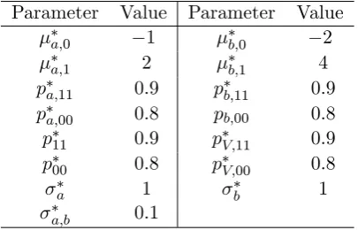
Table 1: Parameter values for generating processes
Parameter Value Parameter Value
a;0 1 b;0 2
a;1 2 b;1 4
pa;11 0:9 pb;11 0:9
pa;00 0:8 pb;00 0:8
p11 0:9 pV;11 0:9
p00 0:8 pV;00 0:8
a 1 b 1
a;b 0:1
[image:31.595.122.474.353.537.2]Note: The table shows the parameter values used to generate the stochastic processes yt in Equation (42) for the simulation study, in Section 2.2.
Table 2: Performance of parameters estimation
z= 1 z= 2 z= 3 z= 4 z= 5 z=f(Vt)
a;0 -0.95143 -0.93985 -0.94558 -0.93750 -0.93166 -0.93896
a;1 1.91921 1.89427 1.90213 1.89147 1.88822 1.89089
pa;11 0.89813 0.89689 0.89729 0.89606 0.89488 0.87803
pa;00 0.79663 0.79508 0.79393 0.78997 0.78900 0.75626
b;0 -1.98915 -1.99861 -1.99591 -1.99903 -1.99503 -1.99729
b;1 3.98711 3.99662 3.99139 3.99859 3.99011 3.99148
pb;11 0.89700 0.89576 0.89581 0.89341 0.89188 0.86977
pb;00 0.79166 0.79155 0.79088 0.78574 0.78600 0.74422
p11 0.89433 0.89241 0.89406 0.89026 0.88991 0.86936
p00 0.78479 0.78295 0.78600 0.77786 0.78900 0.74178
pV;11 — — — — — 0.89682
pV;00 — — — — — 0.80971
Note: The entries in the table report the average of the estimated parameters values through the 1000 replications for di¤erent numbers of synchronization changes, z.
Table 3: Performance of regimes inference
z= 1 z= 2 z= 3 z= 4 z= 5 z=f(Vt)
QP S(Sa;t) 0.05118 0.06448 0.05571 0.06470 0.06023 0.06074
QP S(Sb;t) 0.00749 0.00765 0.00763 0.00829 0.00805 0.00990
QP S(Vt) 0.06387 0.08554 0.09526 0.10988 0.11575 0.17769
Table 4: Dynamic synchronization estimates between New York and Texas
Mean Std. Dev. Median
ny;0 -0.12945 0.01856 -0.12895
ny;1 0.36121 0.01844 0.36079
2
ny 0.02001 0.00153 0.01996
pny;11 0.98322 0.00744 0.98456
pny;00 0.93251 0.02667 0.93539
tx;0 -0.20619 0.02203 -0.20614
tx;1 0.56382 0.02258 0.56399
2
tx 0.02605 0.00187 0.02593
ptx;11 0.98503 0.00642 0.98598
ptx;00 0.93265 0.02687 0.93487
ny;tx 0.00819 0.00156 0.00820
p11 0.98113 0.00775 0.98240
p00 0.93069 0.02523 0.93472
pV;11 0.96516 0.03974 0.97721
pV;00 0.96206 0.02731 0.96879
Note: The selected example presents the case of two states with high and similar U.S. GDP share, New York with 7.68%, and Texas with 7.95%.
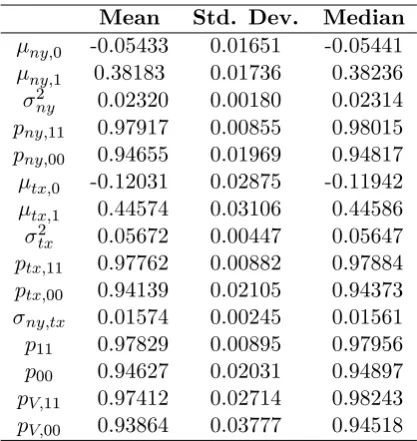
Table 5: Dynamic synchronization estimates between California and Vermont
Mean Std. Dev. Median
ny;0 -0.05433 0.01651 -0.05441
ny;1 0.38183 0.01736 0.38236
2
ny 0.02320 0.00180 0.02314
pny;11 0.97917 0.00855 0.98015
pny;00 0.94655 0.01969 0.94817
tx;0 -0.12031 0.02875 -0.11942
tx;1 0.44574 0.03106 0.44586
2
tx 0.05672 0.00447 0.05647
ptx;11 0.97762 0.00882 0.97884
ptx;00 0.94139 0.02105 0.94373
ny;tx 0.01574 0.00245 0.01561
p11 0.97829 0.00895 0.97956
p00 0.94627 0.02031 0.94897
pV;11 0.97412 0.02714 0.98243
pV;00 0.93864 0.03777 0.94518
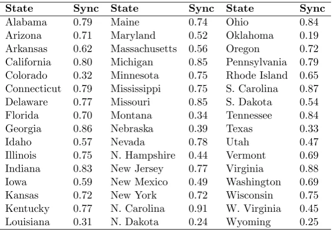
[image:32.595.193.402.480.701.2]Table 6: Stationary synchronization between states and U.S.
State Sync State Sync State Sync
Alabama 0.79 Maine 0.74 Ohio 0.84
Arizona 0.71 Maryland 0.52 Oklahoma 0.19
Arkansas 0.62 Massachusetts 0.56 Oregon 0.72
California 0.80 Michigan 0.85 Pennsylvania 0.79
Colorado 0.32 Minnesota 0.75 Rhode Island 0.65
Connecticut 0.79 Mississippi 0.75 S. Carolina 0.87
Delaware 0.77 Missouri 0.85 S. Dakota 0.54
Florida 0.70 Montana 0.34 Tennessee 0.84
Georgia 0.86 Nebraska 0.39 Texas 0.33
Idaho 0.57 Nevada 0.78 Utah 0.47
Illinois 0.75 N. Hampshire 0.44 Vermont 0.69
Indiana 0.83 New Jersey 0.77 Virginia 0.88
Iowa 0.59 New Mexico 0.49 Washington 0.69
Kansas 0.72 New York 0.72 Wisconsin 0.75
Kentucky 0.77 N. Carolina 0.91 W. Virginia 0.45
Louisiana 0.31 N. Dakota 0.24 Wyoming 0.25
Note: The table reports the stationary synchronization for the period 1979:8 - 2013:3. Those estimates correspond to the ergodic probability that the phases of the state business cycles and U.S. business cycles are the same, i.e. Pr(Vt= 1). The index used to measure