A 3D Computer Vision System in Radiotherapy Patient Setup

Department of Physics and Astronomy, University of Canterbury,

Private Bag 4800, Christchurch, New Zealand

A 3D Computer Vision System in

Radiotherapy Patient Setup

Te-yu Chyou

A thesis submitted in partial fulfillment of the requirements for the

degree of Master of Science at the University of Canterbury

i

Abstract

An approach to quantitatively determine patient surface contours as part of an augmented reality (AR) system for patient position and posture correction was developed.

Quantitative evaluation of the accuracy of patient positioning and posture correction requires the knowledge of coordinates of the patient contour. The system developed uses the surface contours from the planning CT data as the reference surface

coordinates. The corresponding reference point cloud is displayed on screen to enable AR assisted patient positioning. A 3D computer vision system using structured light then captures the current 3D surface of the patient. The offset between the acquired surface and the reference surface, representing the desired patient position, is the alignment error.

Two codification strategies, spatial encoding, and temporal encoding, were examined. Spatial encoding methods require a single static pattern to work, thus enabling

dynamic scenes to be captured. Temporal encoding methods require a set of patterns to be successively projected onto the object, the encoding for each pixel is only complete when the entire series of patterns has been projected.

The system was tested on a camera tracking object. The structured light

reconstruction was accurate to within ±1 mm, ±1.5 mm, and ±4 mm in x, y, and

z-directions (camera optical axis) respectively. The method was integrated into a simplified AR system and a visualization scheme based on z-direction offset was developed. A demonstration of how the final AR-3D vision hybrid system can be used in a clinical situation was given using an anatomical teaching phantom.

ii

iii

Acknowledgement

iv

Table of Content

Chapter 1 - Introduction 1

1.1. Background 1

1.2. Existing Augmented Reality System 3

1.3. Surface Measurement Systems 5

1.4. Project Aim and Outline of Approach 7

Chapter 2 - Structured Light: Theory and Method 9

2.1. Triangulation 9

2.2. Codification Techniques 11

2.3. Camera Calibration 14

2.3.1. Coordinate Systems 14

2.3.2. Camera Model 15

2.3.3. Calibration Theory 16

2.3.4. Calibration Procedure 18

2.4. Projector Calibration 20

2.5. Temporal Encoding Implementation 24

2.6. Spatial Encoding Implementation 25

2.7. Structured Light Reconstruction 30

2.8. Summary 33

Chapter 3 – Structured Light: Accuracy 34

3.1. Capturing a 3D planar surface 35

3.1.1. Method 36

3.1.2. Result 38

3.1.3. Estimating Camera Tracking Error 44

3.2. Characterizing SL 3D reconstruction 44

3.2.1. Method 45

3.2.2. Result 48

3.3. Improved Camera/Projector Setup 52

3.3.1. Improving Calibration Accuracy 52

3.3.2. Modifying Camera/Projector Positioning 54

v

Chapter 4 - Visualization and Full System Setup 58

4.1. Visualization 58

4.1.1. Description and Justification 59

4.1.2. Implementation of the Method 61

4.2. Full System Setup 66

Chapter 5 - Infrared 3D Vision 74

Chapter 6 - Conclusion and Discussion 6.1 Summary and Discussion

6.2 Limitations of the Approach 6.3 Further Work

6.4 Conclusion

78 78 78 80 80

1

Chapter 1

Introduction

1.1 Background

In clincal oncology, there are three principal modalities for treating malignant tumours: surgery, chemotherapy, and radiotherapy [1, 2]. External beam

radiotherapy is a non-invasive procedure that uses ionizing radiation to produce biological damage of cells in the target volume. Cells are damaged by radiation either directly through Coulomb interactions with critical structures such as the DNA, or indirectly through the diffusion of radiation induced free radicals, into critical structures of the cells [1, 2].

The outcome of treatment depends on the response of the tumour cells to ionizing radiation. Ideally, tumour cells should receive irreversible damage that leads to reproductive failure and cell death, thus halting proliferation of the malignant growth [2]. The effectiveness of ionizing radiation in achieving this may be represented by means of the tumour control probability (TCP). In general, TCP increases with dose, however higher radiation doses also lead to more damage to healthy tissues, particularly around the proximity of the tumour. The impact of ionizing radiation on healthy tissue may be expressed by the normal tissue complication probability (NTCP).

The goal of radiotherapy treatment planning is to achieve the highest possible TCP while maintaining NTCP below approximately 5%. The ratio of TCP to NTCP is called the therapeutic ratio, typically in radiotherapy, this should be as high as possible.

2

The standard method for patient alignment on the treatment couch is through use of skin marks placed at the time of treatment simulation and treatment planning. The markers indicate the location of the treatment isocenter. During patient setup the same isocenter position can be reproduced by aligning each skin mark to the appropriate room laser [1, 2].

A significant contributing factor to radiotherapy incidents has been patient

positioning related errors, the most common being inaccurate alignment whereby geographical misses of the target area by several centimeters resulted in unintended doses to healthy tissue [4, 5, 6]. Misalignment of the patient on a bigger magnitude, for example left/right and anterior/posterior confusions have also been reported [6].

In treatment, radiation is typically delivered in fractions for radiobiological reasons to improve the therapeutic ratio [3]. One source of error in this process is the

discrepancies between the patient position and postures during the CT scan and treatment planning, and those during the actual treatment sessions. Since a

treatment can consists of 30 or more fractions, daily patient setup errors can add up and decrease the overall quality of the treatment. At present, on-line MV and kV x-ray imaging is a widely accepted practice for patient setup in radiotherapy.

Electronic portal imaging devices (EPID) use either a metal plate-phosphor screen combination, or a matrix of liquid filled ionization chambers along the linac beam line to produce beam's eye views (BEV) [1]. Portal images can be compared to digitally reconstructed radiographs (DRRs) from the treatment planning system and

treatment simulation to verify the position of the treatment isocenter.

Gantry-mounted kV imaging systems are becoming a key feature in modern medical accelerator design [7]. Unlike MV EPID, gantry-mounted kV systems such as Elekta's Synergy XVI and Varian's On-Board Imager (OBI) use a separate kV x-ray tube

mounted on the gantry, orthogonal to the linac treatment head and any EPI systems associated with it. Gantry-mounted kV imaging systems can perform radiography, fluoroscopy and most importantly, the in-room cone beam computed tomography for volumetric assessment.

3

compared to planning CT data and the treatment couch is translated and rotated to achieve the desired position in a procedure known as rigid-body transformation. One of the shortcomings of the rigid-body transformation based setup approach is that patient deformations, or changes in posture, due to incorrect positioning or changes in the anatomy due to swelling or weight loss cannot be easily detected and

corrected.

A variety of photogrammetric systems have been proposed and tested for the purpose of detecting and reducing planning-to-setup, and treatment-to-treatment positioning errors. The majority of existing systems is either stereovision based [8, 9, 10, 11, 12, 13], or utilizes on-patient markers [14].

In rigid-body transformation, the entire patient is shifted to align the target volume, without posture adjustment. However, of the human anatomy, only bony structures and structures rigidly related to bone can be accurately modeled as rigid bodies. For other parts such as the prostate and the breast, position of the organ and the state of the surrounding anatomy are affected by breathing motion [15, 16] and posture [17]. Furthermore, the typical patient setup procedure involves the use of skin marks to assist day-to-day setup [1, 18], however, the skin itself is not a rigid structure and can vary through the course of the treatment as the result of obesity, variations in muscle tone, or patient posture [18]. Rigid-body transformation should ideally be used with posture corrections to minimize the geometric offset from geometry used in

treatment planning.

1.2. Existing Augmented Reality System

Augmented Reality (AR) has been proposed by our group at the University of

Canterbury and investigated as a means to provide visual guidance during patient set up [19]. AR is a form of computer virtual reality in which real world elements

captured by camera are enhanced by the addition of computer generated graphics. A brief overview of the existing AR system [19] is given here.

The surface contour of the patient is obtained from the patient's pre-treatment CT scan, which is already the standard practice in 3D external beam radiotherapy. The contour data is available as a DICOM-RS object. DICOM (Digital Imaging and

Communications in Medicine) is the standard file format for storing and transferring images between medical equipment. A DICOM-RS object, where RS stand for

4

definitions in radiotherapy. The volumes of interest usually include several levels of treatment target volumes (e.g. GTV, CTV, PTV) defined by the clinician, the critical structures, as well as the body outline of the patient. A Matlab script is used to specifically extract the surface contour from the DICOM-RS object. The contours are then rendered into a surface using Meshlab [20], a 3D surface rendering program.

A registration cube (see Figure 1.1), similar to those used in the routine quality assurance (QA) of CT alignment lasers, is used to register the camera location and orientation with respect to the linac isocenter. The registration cube is positioned on the treatment couch, with the aid of the room laser, such that its center coincides with the linac isocenter. A single view of the registration cube by a calibrated camera (see section 2.3) is sufficient for the required transformation parameters to be determined. The transformation parameters can then be used to display the 3D model of the patient outline on top of the live camera view of the linac. The cube can be removed once the registration process is done, and patient set-up may begin. During the alignment of the patient, the radiation therapists now have the option to refer to the augmented monitor with the correctly positioned contour on-screen (see Figure 1.2).

5

Figure 1.2. Augmented monitor with the correctly positioned contour on-screen in the existing AR system [19].

The accuracy of the AR system in a clinical environment was evaluated

experimentally using an anthropomorphic phantom. The phantom was positioned on the linac treatment couch based on the on-screen contour. A CBCT scan of the

phantom in its final position was taken, and compared to the CT volume. From the measured offsets between the CT and CBCT volume, a translational error of 3mm, and rotational errors of 0.19o, 0.06o and 0.27o in pitch, roll and yaw respectively, were deduced.

While AR can provide a visualization of optimal patient surface contour for posture adjustment and aid in rigid-body transformation, it remains a visualization tool and provides no quantitative information. To quantify offsets from the optimal contours caused by posture related deformations, recovery of the actual patient contours is necessary so comparison to planning CT data can be made.

1.3. Surface measurement systems

In external beam radiotherapy, high precision in target positioning relative to the treatment planning coordinate system is imperative to the success of treatment. Patient surface tracking has received growing attention in recent years and

commercial products specifically designed for radiotherapy patient monitoring have been developed. The most well known is the stereovision based system, AlignRT [21] by VisionRT.

Bert et al (2005) [11] studied AlignRT's capability in detecting patient shift. In their work on patient realignment, a mannequin phantom was set up on the treatment couch, the couch was then purposely misaligned with the new coordinates

6

AlignRT to calculate the transformation required to realign and compared the result to the known transformation. In 54 sets of random couch coordinates, the biggest translational error was 0.75 mm and the biggest rotational error was under 0.1o. Given that the roof mounted pods were 2.7 m away from the phantom and the resolution of the cameras being 1024 by 768 pixels, the hardware could not have achieved sub millimeter spatial resolution (due to the likely size of the field of view, and the relatively small number of available camera pixels), thus demonstrating the importance of optimization software.

AlignRT has since been tested in cranial stereotactic radiotherapy (SRT) and radiosurgery (SRS) [8, 10], which require some of the most accurate and precise patient alignment amongst the present external beam treatment techniques. In one of the studies, AlignRT produced alignment accuracy comparable to current

image/marker-based systems [8].

Computer stereovision relies on two or more distinct, two dimensional digital images of the same object to extract three dimensional information. The simplest form of stereovision is the binocular stereo. Binocular stereo uses two identical cameras positioned such that the image planes of cameras are parallel to each other, and the camera centers are at the same height. Recovering depth information involves two key steps, solving the correspondence problem, and calculating the depth from the disparity [22, 23, 24]. For a single point on the object, disparity refers to the

difference in position of this point on the respective image plane of each camera. Disparity is inversely proportional to depth and enables the computation of a 3D representation of the object.

One of the main challenges in building a stereovision based 3D surface imaging system is to solve the correspondence problem. Correspondence problem arises because each point on the image seen by one camera has a line of possible choices (the epipolar line) for the corresponding point as seen by the other camera [22, 23, 24]. Correspondence problem is solved by sliding a window along the epipolar line. Correspondence is where pixels within the corresponding windows have similar intensity. Solving the correspondence problem directly can be difficult when the object of interest is the human body. The skin is in most cases featureless and the matching method is therefore susceptible to false matches.

7

Because the illumination is coded, correspondence between image points and points on the projected pattern can be identified. The process of finding correspondences is known as decoding of the structured light [25, 27], once the captured image points are decoded, the 3D information of these points can be established through

triangulation [25].

1.4. Project Aim and Outline of the Approach

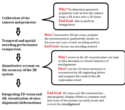
The aim of this project is to implement a structured light based 3D surface measuring technique, then customize and integrate the 3D vision technique into the existing AR approach. The final setup guidance system uses AR to provide a visualization of the optimal patient position and posture for initial positioning. The accuracy of the positioning is then determined quantitatively using the 3D surface measurements (refer to Figure 1.3). The ideal system should provide quantitative information on misalignments on a region-to-region basis, instead of the global correctness of the alignment. This feature is important, it provides the user with the location and the magnitude of a misalignment caused by a localized deformation.

Figure 1.3. Roles of the AR and 3D vision system in the workflow of a typical external-beam radiotherapy treatment course.

8

9

(2.1)

(2.2)

Chapter 2

Structured Light: Theory and Method

2.1. Triangulation

In a homogenous medium such as air, light traverses in straight lines. Every pixel on a camera image defines a camera ray. A camera ray describes the direction in which a light ray must be incident upon for it to be registered by that camera pixel. It is represented geometrically as a straight line (see equation 1) in 3D space that passes through: 1. the focal point of the camera; 2. the location in the scene from which the light originated. Let p be the coordinate of a point in the scene, the vector equation of a camera ray crossing this point takes the form of a straight line:

where v is the direction vector and v0 is a point on the line and u is a scalar.

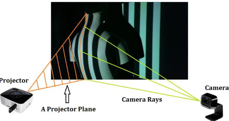
A projector works like the inverse of a camera. A dot projected onto the scene forms a projector ray between the focal point of the projector and the point of intersection with objects in the scene. Similarly, a line projected onto the scene, forms a 3D projector plane that contains the focal point and all points on the line segment illuminated by the projection (see Figure 2.1). The equation for a projector plane is:

10

(2.3) Figure 2.1. Relationship between a projector plane and camera rays. Each stripe pattern projected onto the scene can be thought of as a 3D plane intersecting with object in the scene. When a camera sees the illuminated stripe, the position of each of the illuminated pixels on the image plane relative to the focal point defines the camera rays which form the camera image of the stripe.

11

2.2. Codification Techniques

For triangulation to work, each camera ray must be intersected with the correct projector plane. To achieve this, the projector must illuminate each part of the scene differently to make regions in the scene distinguishable on the camera images. This step is known as encoding.

Encoding patterns can be divided into two main categories [25]. The temporal encoding techniques, which are characterized by the use of a sequence of encoding patterns, and the spatial encoding techniques that use a single pattern to encode the scene.

In temporal encoding, each part of the scene is given a unique codeword in the form of a colour sequence. The encoding is done by projecting a sequence of patterns onto the scene using a data projector or similar illuminating devices. Since only one pattern can be projected at any instance, the minimum number of camera frames required to capture the whole sequence is the number of encoding patterns. This feature gives the method its name of temporal encoding. The maximum resolution of the system is constrained by both the camera and the projector resolution. The maximum number of codewords that can be generated by a data projector is the number of projector pixels. In the situation when the camera used has a much better resolution, a group of neighbouring pixels on the camera captured sequence may share the same codeword, these groups of neighbouring pixels will be referred to as

encoding regions for the remainder of the thesis.

12

Figure 2.2. A simple binary code (top) compared to Gray code (bottom). Notice that when certain sections (for example the blue boxes in the middle panel) of a simple binary code is reflected in a specific manner (indicated in red on the right of each section), a binary Gray code is produced.

13

Figure 2.3. Section of a spatial encoding pattern (taken from [28]) based on a De Bruijn sequence with subsequence length of 3 (left), and the same pattern projected onto an object (right). Notice that the codeword for each encoding region (vertical stripes) is not unique on its own. For example, the colour yellow is used in four encoding regions. If however, the encoding regions are examined in groups of three, none of the combinations are repeated.

Besides the two main categories, there are also direct codification strategies that use a large number of either colours or grey levels so that the entire scene can be

14

2.3. Camera Calibration

2.3.1. Coordinate Systems

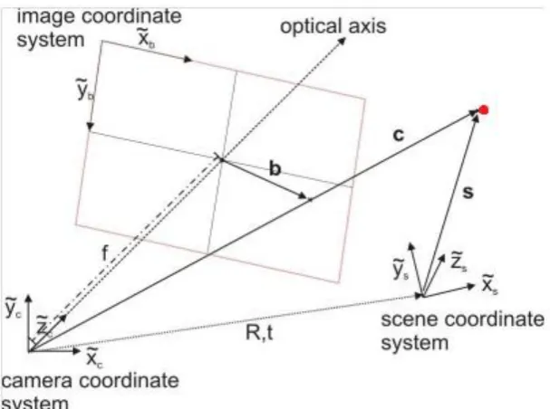
In the mathematical model of projecting a 3D point in world coordinates onto the image plane of a pinhole camera, the position of the point on the image depends on: (1) where and in what orientation the camera is relative to the point, and (2) the internal geometry of the camera. Three coordinate systems involved in this model are: the world (or scene) coordinate system, the camera coordinate system, and the image coordinate system (see Figure 2.4).

The world coordinate system can be chosen in any convenient way. The coordinate of an object in the room is a relative quantity, it depends on where the origin is and how the axes are orientated, however, the relative positions between objects remain unaffected. The choice of the world coordinate system therefore makes no difference to the final image taken by the camera.

The camera coordinate system is a three-dimensional coordinate system centered on the focal point of the camera. In this project, the Z-axis is always the optical axis of the camera, and the X and Y axes are positioned accordingly. The transformation from world coordinates into camera coordinates is linear, and can be calculated explicitly with the aid of a registration cube, or using calibration patterns.

15

Figure 2.4. Coordinate systems. The bald red point can be shown in three different coordinate systems, in world coordinates (vector s), in camera coordinates (c), or in image coordinates (b)

2.3.2. Camera Model

The objective of camera calibration is to determine the parameters that describe the mapping between 3D world coordinates and the 2D image coordinates [30, 31]. The set of parameters that maps 3D camera coordinates onto 2D image coordinates is known as the intrinsic parameters. Intrinsic parameters represent the camera's internal geometric and optical characteristics, these include: focal length, principal point, skew coefficient, and distortions [25, 33]. Parameters that determine the mapping from world coordinates onto camera coordinates are the 6 extrinsic parameters, 3 for the Euler angles for rotation around the x, y, and z axes of the world coordinate system, and 3 for translations in the x, y, and z directions, respectively [32, 33].

(2.4)

16

axis orientation (look angle) of the camera with respect to the world coordinates, and the fourth column t is the 3D displacement vector of the camera focal point and the origin of the world coordinates. In the intrinsic matrix A, f is the focal length of the camera, it is presented in pixel units and appears twice in the intrinsic matrix to deal with non-square pixels (i.e. aspect ratio), Cx and Cy are the position in pixel unit,

of the central point of the image (called the principal point), where the origin is the top left corner of the image by convention. αc is the skew coefficient which defines

the angle between the x and y pixel axes, for most cameras this angle is close to 90 degrees leading to a zero value (or very close to zero), that is why in some calibration model the estimation for skew coefficient is skipped.

If X, Y, and Z are row vectors containing in world coordinates, the x, y, and z

components of surface points of a 3D object, equation 2.4 then describes the perspective projection of a 3D object. Perspective projection is one of the most important underlying principles in Augmented Reality. It is the process of determining how a 3D object would appear on camera, given the intrinsic

parameters of the camera, and the position and orientation of the camera relative to the object. It is important to note that while projecting a given 3D scene coordinate onto the image plane is straight forward using 2.4, the reverse (i.e. 3D vision, the recovery of 3D coordinates from image coordinates) cannot be achieved using this equation alone.

2.3.3. Calibration Theory

The camera was calibrated using Bouguet's Camera Calibration Toolbox [34]. The toolbox is largely based on Zhang's method [33]. Zhang's method begins with the estimation of the homography relating image points and points on the calibration plane, the closed-form solution for the intrinsic and extrinsic parameters are then calculated from the homographies. The radial distortion coefficients are then solved using linear least-squares, and finally, every parameter calculated is refined through maximum likelihood estimation.

The specific method uses 2D external patterns in the form of checkerboards to provide the set of points in world coordinates. The camera model described by 2.4 can be simplified if the Z = 0 of the world coordinate system is chosen to coincide with the checkerboard, in this case, we may drop the third component from the vector for the scene point, and the third column of the 3 by 4 extrinsic

17

Furthermore, let

(2.5)

so (2.1) becomes

s

m

= H

M

m

= [

u

,

v

, 1]

M

= [

X

,

Y

, 1]

Matrix H is known as the homography, which relates 3D scene points and the 2D image of the scene. The homography is estimated in the calibration toolbox using a technique based on a maximum likelihood criterion [34].

Because rotation matrices have linearly independent unit vectors as columns, vectors r have the properties:

From (2.5) and the above conditions yield two constraints on the intrinsic matrix A:

18

2.3.4. Calibration Procedure

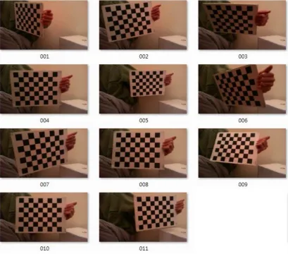
A 9 by 7 checkerboard was used for calibration. The calibration board was made of printed checkerboard pattern pasted on a flat panel, and each square measured 30mm x 30mm. The calibration board was held in front of the webcam over a range of distances and rotation angles (see Figure 2.5). For each calibration board

orientation, a 1200 x 768 pixels image was acquired and saved as a jpg file. After at least ten calibration patterns were acquired, the calibration toolbox was run under Matlab to process the saved calibration images.

Figure 2.5. Calibration using a checkerboard pattern.

The calibration toolbox did not automatically detect the grid corners. For each image the four extreme grid corners must be selected manually, the toolbox could then search for all remaining grid corners automatically (see Figure 2.6) using a built in corner detecting algorithm. The grid corners found were in 2D image coordinates (u,

19

origin, and the coordinates for all other grid corners were found by adding the appropriate integer multiples of the grid corner spacing in X and Y (with Z = 0 on the board, see section 2.3.3).

The selection of the extreme corners was done by clicking of the mouse, the corner detector helped minimize the clicking error, as long as the mouse click was no more than 5 pixels away from the true corner. The first clicked point was automatically chosen to be the origin of the world coordinate system. The choice of the first point is of particular importance in a multi-camera system. In multiple camera calibration, each calibration board orientation has a set of corresponding calibration images (one image for each camera), and the same first point must be clicked on all images across the set to accurately estimate the relative positions of the cameras. Figure 2.7 is a visualization of the extrinsic camera calibration result.

20

Figure 2.7. For each calibration image, a set of extrinsic parameters can be estimated. enabling the recovery of checkerboard location at the time of image acquisition. In the figure, the axes of the camera coordinate system are shown in the blue with the point Oc being the origin as well as the focal point. Colored grids numbered 1-11 are

the estimated locations of the checkerboard featured in the Figure 2.5

2.4. Projector Calibration

LCD projectors work by splitting a strong white light source into the primary colours through a prism, then onto small LCD panels. These panels control the amount of red, green, and blue light that can pass through each pixel on the panels. When the light passing through the LCD panels are recombined, a 2D image is formed. This location inside a projector is analogous to the image plane of a camera, and for the sake of simplicity, it will be known as the image plane of the projector from here on. From the image plane, the recombined image is then projected onto the scene through divergent lenses.

21

Mathematically, equation 2.4 is therefore also valid for projectors.

The calibration procedure for a projector is in principle similar to that of a camera, the key differences lie with the design and function of the calibration board and the extra step required in the software. Projectors cannot capture images of a

checkerboard, so instead a checkerboard pattern is projected onto a plain board. Grid corners of the projected checkerboard are used as scene points for calibration. Unlike the printed checkerboard used in camera calibration, the dimensions of the projected checkerboard pattern depend on the relative positions of the calibration board and projector. The 3D position of the grid corners, in the world coordinate system therefore cannot be simply assigned for like in camera calibration.

One way to calculate the grid corners is to attach points of reference to the

calibration board so the position and orientation of the calibration board is known [25]. This is essentially a camera extrinsic calibration. From the knowledge that the grid corners lie on the plane, 3D coordinates of the projected grid corners can be found using either a ray-plane intersection or a perspective transformation based method. At this point, there are two choices of coordinate systems for the 3D coordinates:

1. In world coordinates - choose one of the four reference points (the four fiducial markers in Figure 2.8) as the origin, let the calibration board coincide with the Z = 0 plane, assign coordinates to the three other known reference points, then use the perspective transformation to calculate the corner coordinates of the projected checkerboard.

2. In camera coordinates - use a calibrated camera to look at the calibration board, calculate the extrinsic parameters from the four reference points using the

calibration toolbox, this gives the translation and rotation of the calibration plane relative to the camera. Then either apply the transformation after calculating the world coordinates using option 1, or build direction vectors for 3D rays going through the grid corners, then find the ray-plane intersection for each grid corner.

While presenting the grid corners in camera coordinates requires an extra step in the calculation, it has the added advantage of providing projector position and

22

Camera Calibration Projector Calibration

Mathematical Model Equation (2.4) Equation (2.4)

Pixel sizes of grids (u, v) on the image plane

Grids have different sizes All grids have the same size

Dimension of grids (X, Y,

Z) in the actual scene

Grids on the printed checkerboard all have the

same size

Grids on the projected checkerboard have

different sizes Determining grid corners

in image coordinates on the image plane

Measured directly from images using corner

detector

Assigned based on the pixel dimensions of the projected checkerboard Determining 3D

coordinates of scene grid corners

Let Z = 0, first clicked point being the origin, coordinates assigned to the other points because checkerboard dimensions

are known

Calculated from the image coordinates of: 1. fiducials, and 2. grid corners measured by a

calibrated camera

Coordinate system in which scene grid corners

are presented

World coordinates, Z = 0 along the surface of calibration board, origin chosen by first click rule

Camera coordinates, camera focal point is the

origin, Z axis along the camera optical axis Table 2.1. Comparison of camera and projector calibration.

Projector Calibration Procedure

A plain 40 cm by 40 cm board with fiducial markers on the four corners was constructed. The fiducials used were in the form of 2 by 2 checkerboard patterns, they were pasted onto the corners of the board to form a 30 cm by 30 cm square between the grid corners. The remaining area of the board was covered in white (see figure 2.8).

23

A 1024 by 768 image matrix representing a 8 by 8 mono-colored checkerboard pattern in the middle and white background was generated in Matlab. The image was projected onto the calibration board using the Screen function in the

Psychophysics Toolbox. The function Screen converts a Matlab image matrix into input signals for computer displays, and then passes the signal onto the appropriate device according to the user specified screen number (the Psychophysics toolbox automatically detects all display units connected to the computer, and numbers them in integers). Images of the projected pattern were captured for a range of board locations and poses. The method for obtaining the image coordinates of the projected grid corners was identical to the corner extraction procedure in camera calibration: manually select the four extreme corners followed by automated corner detection of the rest. The four reference points for board location and orientation tracking were also manually found with the aid of the corner detector, the image coordinates were then put through the extrinsic calibration function of the calibration toolbox, to determine their 3D locations in camera coordinates.

24

2.5. Temporal Encoding Implementation

The Matlab code used for generating the temporal encoding sequence was primarily based on Lanman & Taubin (2009) [25] with changes made only to the capturing method of the encoded scene.

Lanman and Taubin’s Gray code implementation [25] consisted of all of the patterns that would feature in a binary sequence, as well as the inclusion of the binary

inverses of each binary pattern (see Figure 2.9). The length of the encoding sequence was determined by the resolution of the encoding projections. For example, the length of binary codeword would have to be at least 10 (i.e. 10-bit), to encode an array of 210 = 1024 unique segments, which also means an encoding sequence of at least 10 images would be needed. If the binary inverses were added, the encoding sequence length would double. All-on and all-off images (refer to the first two patterns in Figure 2.9) were introduced in Lanman and Taubin’s implementation to improve decoding accuracy. In decoding, the software assigned every pixel of each captured frame as either lit or not-lit by examining the r-g-b values at that pixel. A threshold value in intensity was therefore required to complete the determination process. A universal threshold value for this had a major drawback: due to geometry of the surface been scanned, the intensity of illumination varies across the scanned surface [25]. This meant an un-lit pixel could be misassigned as an “on” pixel due to scattering of light, and conversely, a lit pixel could be interpreted as an “off” pixel because the surface curved away from the incoming light direction (see Figure 2.10). The all-on/all-off patterns allowed the local illumination intensity to be taken into account when deciding if a pixel was on or off.

25

Figure 2.10. Example of the encoding process, blue represents the path traversed by the lit sections of the encoding pattern and grey represents the un-lit sections. Region 1 on the object surface will have lower illumination intensity than region 2 due to the curvature. Region 3 will appear brighter than the other un-lit regions due to scattered light from region 4.

2.6. Spatial Encoding Implementation

Despite the large amount of available literature on spatial encoding structured light, at the time of this project, a ready-to-use spatial encoding structured light program for Matlab was not available. While some utility functions from Lanman and Taubin’s structured light toolbox, such as those used in triangulation, could be reused for the spatial encoding technique, the majority of the method still had to be programmed. Implementing an efficient and elegant program, particularly for the decoding part, would require a strong background in combinatory theory. This was considered too difficult for the time frame of this project, and a “keep it simple” approach was followed instead, disregarding the importance of efficiency.

2.6.1. Codeword creation

26

the number of characters, and the sub-sequence length, to generate an interleaved pseudo-random De-Bruijn sequence and in the format of an integer array [37]. The numbers were than translated into colours, for example, 1 for the colour red, 2 for green, and 3 for blue. One drawback with this generator, for the purpose of spatial encoding at least, was the immediate repetition of any number in the sequence, For example, one of the six possible De-Bruijn sequences for 3 characters and

sub-sequence length 2 was "121332231". In a codeword, a segment of the same number repeating itself (“33” and “22” in the previous example) would translate the whole neighbourhood of encoding regions into the same colour. This became an issue because it was difficult for the software to distinguish whether a stripe on the camera image was really one stripe or multiple neighbouring stripes all with the same colour. In the last example, the “3322” segment should translate to

“blue-blue-green-green”, but it could easily have been mistaken as (but not limited to) “blue-green”, “blue-blue-green”, or “blue-green-green”.

The computation in the original code used a brute force approach. For a De-Bruijn sequence using n number of characters and k subsequence length, a list of every possible permutations of length k, using only the integers within the range 1 to n, was generated. From the list, one subsequence is randomly chosen at a time, and its first k-1 elements were compared to the last k-1 elements of the current overall sequence. Call the described process Step 1 for convenience and let m be the current overall sequence length. Step 1 was repeated until a match was found and in which case, the matching subsequence was deleted from the list and added to the overall sequence (m to m+1). The software would then loop back to Step 1, to search for the next matching subsequence for the updated overall sequence (now m+1 in length). In the case when no matches could be found for m+2, the program would backtrack by removing the last matched subsequence (m+1 to m) and search for an alternate. Call this Step 2. Step 2 would be repeated if no alternative could be found for m+1, and it was not unusual for the program to keep backtracking until m = 0, in which case a new starting subsequence would be randomly chosen from the list.

27

default finds all combinations of length k, from n things, without using any one element more than once per combination. perm tabulates all possible permutations of a list of numbers, this function was used on each combination found by nchoosek

to generate the full, new list of subsequences under the modified criterion.

The resolution of the webcam used in this project was not high enough to make full use of the projector resolution of 1024-by-768 pixels. The encoded scene occupied from one-third to half of the camera image, which had a resolution of 1280-by-720 pixels, this meant encoding patterns would lose around half of their resolution during capturing of the scene image. The smallest feature on the encoding pattern therefore had to have at least 2 pixels in both dimensions to have a reasonable chance of being seen in its entirety. To avoid misdetection, the stripes on the encoding pattern were set to 5 pixels wide.

2.6.2. Codeword Extraction

The image of the encoded scene was saved in RGB format, each colour channel of a given pixel was stored as an 8-bit unsigned integer (UINT8 format, range between 0 and 255). The colour data for every pixel was converted from RGB, based on a series of colour selection criteria, into integers 1 to n for pixels that passed the selection, where n is the number of colour used, and 0 for those that did not meet any of the criteria. The mean value of the three colour channels was calculated for every pixel, a lower threshold was set based on the mean, and any pixel with a value below the threshold was deemed part of the un-encoded regions or background and was assigned the value 0. For all pixels that passed the brightness filter, ratios of colour channels (e.g. r/g, g/b) were calculated. The colour channel ratios were used for determining the colour of the pixel. As an example, if r/g = 2.23, r/b = 1.92, and b/g = 1.16, the colour assignment for that pixel should be red or the value 1, because the red channel was significantly more prominent than both the green and blue channels. The output from the described colour assignment was a 1280-by-720 matrix that had the same number of representations of colours as those in the original encoding pattern. A global set of criteria was used for colour determination. Colour

28

(a) Encoded scene image

(b) Colour identified from scene image

(c) Colour identification error, leftt: image of the scene, right: identified colours.

29

2.6.3. Decoding

Due to the short length of the codeword (less than 200 elements), the decoding was done through a “brute force” method, by searching for each observed subsequence in the original encoding sequence. The codeword for each row of the image pixels were compared to the original codeword used to generate the encoding pattern. Segments of the codeword indentified from the image were systematically extracted, 4 elements at a time. A vector v, identical in length to the camera captured codeword, and containing the location of each codeword element within the original codeword was calculated. Let m be the length of the imaged codeword, n the length of the original codeword, y the index for elements of the imaged codeword, and x the index for elements of the original codeword, the steps for finding correspondence between the two code-words were as follows:

1. The first 4 elements of the codeword segment (y = {y0, y0+1,..., m-1, m}) were

extracted to form a subsequence, a matching subsequence was searched for in the original codeword. Let x = x0 be the vector index of the first element of the

segment in the original codeword that matched the subsequence, the location of this subsequence would be x0, x0+1, x0+2, x0+3.

2. Compare every subsequent element of the segment (that is, y = y0+j, where y0 is

the vector index of the first element of the segment from the captured codeword, and j = {4, 5, ..., m- y0}) to the corresponding elements of the original codeword

(i.e. x = x0+j), proceed until either (a) a mismatch was encountered or (b) all

elements of the segment were matched to the original codeword. In the latter case, skip Steps 3 and 4.

3. If a mismatch between the imaged and original codeword occurred, it was likely due to a jump in the imaged codeword caused by steep surfaces. In this situation, the segment starting on the element mismatched would be extracted by setting the current y to y0 and return to Step 1.

4. If a new starting point in the original codeword could not be found, the

mismatched element seen in Step 3 was probably the result of either an error in colour identification, or the encoding region was too narrow to be encoded by a complete subsequence of 4 coloured stripes. This element in the imaged

30

5. Every element of the imaged codeword should now have either a corresponding element in the original codeword, or been flagged as unidentifiable.

2.7. Structured Light Reconstruction Results

A test scene was constructed out of simple 3D shapes, these included a cylinder, a square box, and a polystyrene container with rectangular blocks of varying sizes cut off (see Figure 2.12). All of the objects in the scene were made white to minimize the effect of intrinsic surface colouration on spatial encoding. Both the temporal and spatial encoding techniques were used to reconstruct the scene.

Figure 2.12. First test scene for the structured light 3D vision methods.

31

(a) projector columns recovered from the temporal method.

(b) projector columns recovered from the spatial method, black boxes showing regions where decoding error occurred.

Figure 2.13. Decoded projector column indices displayed in colour, ranging from dark blue for column 1, to dark red for column 1024

The reconstructions of the scene are shown in Figure 2.14, features on the

32

33

2.8. Summary

A 3D structured light system was setup and tested. Both the temporal and spatial encoding strategies were trialed. Temporal encoding technique based on Lanman and Taubin (2009) [25] required a sequence of 42 images to encode the scene, the encoding time requirement was compensated by the robustness of the method under non-ideal lighting conditions. The spatial encoding technique implemented required only one image of the encoded scene to produce a 3D reconstruction, however, the simple colour recognition procedure implemented was highly

susceptible to detection error. The colour stripes were made wider and interleaved in order to reduce detection error, however, this also lowered the spatial resolution.

The two structured light methods differed only in their encoding and decoding techniques. If the techniques were on-par in decoding accuracy and resolution, then they should, in principle, have the same 3D reconstruction error. In reality however, the simplified spatial encoding implementation could not achieve the same level of accuracy and resolution as the temporal method. The temporal encoding technique was therefore deemed the better choice for testing the accuracy of the structured light method. Figure 2.15 is a qualitative preview of the capability of the 3D vision method using structured light temporal encoding.

34

Chapter 3

Structured Light Accuracy

Offsets between captured 3D patient surfaces and CT data sets can have any or all of the following four origins: (1) Patient movement, change in posture, (2)

misalignment/error in patient setup, (3) Inaccuracy in camera tracking, (4) Inaccuracy in the measured 3D surface. Out of these four types of offsets, (1) and (2) is what the 3D vision system sets out to detect i.e. the true offset of patient position and pose, (3) and (4) are errors that should be minimized.

Inaccuracy in camera tracking will generate error in the transformation between camera and world coordinates, this error will in turn cause the planned patient surface contours to be misplaced in camera coordinates.

Inaccuracy in the measured 3D surface refers to any offsets caused by the 3D vision system, measured when both type (1) and (2) offsets have been eliminated.

Quantifying errors (3) and (4) separately was technically challenging. In the existing AR system, the tracking error (type 3) was thought to be only in the rotational parameters. It was estimated that the camera tracking procedure had rotational errors of 0.5o in roll, pitch and yaw. To put this error into context, if a registration cube of 9.5 cm sides was positioned on the linac couch using the room laser setup approach [19], with an intentional 0.5o offset in yaw, the maximum misalignment between the sagittal room laser and the z-axis of the cube would be 0.4 mm. Due to the finite laser beam width and temperature influences, it is difficult to directly measure errors of this magnitude. This is reflected on the 1 mm laser accuracy tolerance recommended by IPEM [38], and AAPM [39] for stereotactic procedures [39] that demand the highest level of accuracy.

35

It is also worth noting that, the terms extrinsic camera calibration, camera tracking, and camera registration are used synonymously, they all refer to the procedure of calculating the camera's extrinsic parameters from the corners of a checkerboard pattern with known dimensions (see section 2.3). The terms tracking board,

calibration board, and tracking device all refer to the same board seen in Figure 2.8, which is analogous to the registration cube used in the original AR system. The board was previously used for projector calibration. In this chapter however, it was used as a test object for 3D reconstruction while simultaneously serving as the object for camera registration.

3.1 Capturing 3D surface of a plane

In this experiment, the 3D surface of a plane was captured. The goal was to

36

3.1.1. Method

The camera and projector system was calibrated and fixed in one location throughout this experiment. The object plane was placed 1 m in front of the vision system, the room light was then switched off and the surface of the plane scanned using the temporal encoding structured light sequence. The first image of the encoding sequence (the all 'on' image) was also used for extrinsic camera calibration. The experiment was repeated for three different plane orientations: rotations of -10o, 10o and 35o pan angle (about the y axis). A 13 degree tilt angle had to be added so the board could lean against the supporting stand behind.

The four fiducial corners on the each reconstructed 3D point cloud were identified manually. This task turned out to be simple because the square patches on each fiducial marker were black and could not be encoded and were shown on the

reconstruction as square holes (see Figure 3.1a). Where the corners of two holes met (i.e. the region enclosed by the red circle in Figure 3.1a) was taken as one of the board corners.

37

(a)

(b)

Figure 3.1. (a) 3D plot showing the reconstructed point cloud zoomed in on the top left. The holes made the corner to be easily identifiable. (b) A photo of the

38

3.1.2. Results

The coordinates of the corners found from the structured light scan and extrinsic calibration were compared and significant discrepancies were observed. The distances from the front of the camera to the fiducial markers on the board were measured directly with a tape measure and compared to the vision based

measurements. There were discrepancies in measured camera distance between all three measuring techniques. To characterize the type of discrepancy between the techniques, an offset value was calculated at each corner, using measurements from all three plane orientations. Table 3.1 is a summary of the results.

Corner 1 Corner 2 Corner 3 Corner 4 Directly measured

and camera tracked

14 ± 1 13 ± 1 12 ± 2 12 ± 1

Directly measured and 3D reconstructed

-12 ± 8 -4 ± 5 10 ± 5 8 ± 3

Camera tracked and 3D reconstructed

26.3 ± 7.4 16.5 ± 4.0 2.6 ± 4.7 3.8 ± 2.8

Table 3.1. Difference in camera to corner distance measurements (in mm) between different techniques, values shown are the mean and standard deviation of

measurements from the three plane orientations.

39

In the structured light 3D reconstruction, the distance measurements of the corners were less consistent with the direct measurements. The offset ranged from 12 mm closer to the camera at corner 4 to an extra 10 mm away at corner 2. When

compared to camera tracking/extrinsic calibration, the offset ranged from 26 mm at corner 4 to 2.6 mm at corner 2. In the construction of the calibration board, the fiducial markers were carefully positioned so their centers would form a 299 mm by 299 mm square, these can also be measured from the structured light reconstruction by finding the magnitude of the difference vector between each non-diagonal pair of corner coordinates (see Table 3.2).

Side 1 Side 2 Side 3 Side 4

Orientation 1 (red)

302 304 298 306

Orientation 2 (magenta)

301 309 298 314

Orientation 3 (blue)

302 299 299 297

Table 3.2. Measurements of side lengths (in mm) of a 299 mm by 299 mm square using the structured light method, a visualization of the three plane orientations can be found in Figure 3.2, the sides are numbered in clockwise direction starting on the lower left corner (refer to the green markers in Figure 3.2). Colour references are made to the marker colours in Figure 3.2.

The structured light reconstruction had distortions in dimensions, it was most accurate on Side 3 for all three orientations, with less than 1 mm error, and most inaccurate on Side 4 with up to 16 mm in error. The distance measurements of the two corners (3 and 4) forming side 3 of the square were also in better agreement with distances found by camera tracking. This observation was in agreement with theory. Regardless of the structured light reconstruction accuracy, the perspective projection of the recovered corners back onto the image plane should always coincide with the pixel coordinates of the fiducial markers. That is, if the

40

Figure 3.2. The four corners of the board in camera coordinates obtained from

41

Figure 3.3. Relationship between camera rays (black lines) and points in the scene (blue crosses). In this example every camera rays passes through six grid patterns in the scene, while all six grids have different sizes, they should all project onto the same pixel coordinates on the image plane.

42

The same projection test was also performed on the 3D coordinates recovered from extrinsic calibration. For these coordinates, the problem of choosing the right points from the point cloud was eliminated because each of them was originally derived from the pixel location of a fiducial corner. The task was therefore simplified down to the mapping the 3D coordinates onto appropriate pixel positions using equation 2.4. Despite eliminating the two possible sources of error stated in the previous

paragraph, the discrepancies from the fiducial corners were still between 0.6 to 2.3 pixels (see Figure 3.5) which corresponded to a physical distance of around 0.5 to 2.0 mm on the board. An explanation for this was the discrepancies between the

algebraic forward mapping (i.e. taking a photo of the scene) of 3D camera coordinates onto 2D pixel coordinates, and the numerical inverse mapping (i.e. during camera extrinsic calibration/tracking) from 2D pixel coordinates to 3D camera coordinates. If a camera model free of distortion was used, then the inverse mapping would just be solving for the camera coordinates (i.e. transformation matrix applied to the world coordinates X, Y, and Z) by taking the inverse of the intrinsic matrix A in equation 2.4. In that situation both forward and inverse mapping could be done by an algebraic expression. However with a high degree distortion correction in the camera model [34], the inverse mapping could no longer be described by a simple algebraic expression. In the Camera Calibration Toolbox [34], a numerical model was implemented for extrinsic calibration for this reason.

43

Figure 3.4. Accuracy of intrinsic camera calibration, showing the pixel coordinates of: 1. corners found by the corner detector (Red); 2. the coordinates in red transformed into 3D then re-projected back onto the image (Green); 3. 3D coordinates from SL projected onto the image (Yellow).

Figure 3.5. Discrepancies in pixel coordinates of fiducial corners and of the projected 3D coordinates.

-2 -1.5 -1 -0.5 0

-2 -1.8 -1.6 -1.4 -1.2 -1 -0.8 -0.6 -0.4 -0.2 0

x offset in pixels

y

o

ff

s

e

t

in

p

ix

e

44

3.1.3. Estimating Camera Tracking Inaccuracies

In the previous section, discrepancies were observed when the 3D coordinates recovered by extrinsic calibration were projected (forward mapped) back onto the original image. Pixel coordinates of the re-projected corners were all shifted towards the origin of the image coordinate system. The magnitude of the shift ranged from 0.3 to 2 pixels in the x-direction and 0.4 to 1.5 pixels in the y-direction (see Figure 3.5). The mean offset in x-direction was -1 pixel with a standard deviation of 0.5, in the y-direction the mean was also -1 pixel with a standard deviation of 0.4 pixels. The pixel distance between each pair of fiducial markers in the images ranged between 307 and 381. Based on this information, pixel length was approximated as 0.88 ± 0.10 mm. Using the estimated pixel length and the mean pixel offsets, a physical offset of +0.88 mm in the both x and y directions was applied to compensate for the observed shift. The errors in the 3D coordinates after this correction should be ± 0.60 mm in the x-direction and ± 0.50 mm in the y-direction.

The error in the z-direction was estimated by measuring the pixel lengths of the re-projected sides. Unlike in structured light reconstructions (refer to Table 3.2), the length between 3D corner coordinates recovered by extrinsic calibration would always be 299 mm (it is an input parameter in the extrinsic calibration). This meant the side lengths (in pixels) between the re-projected corners could only be in agreement with side lengths of the fiducial markers if the calculated distances to camera were also in agreement with the true distances to camera. Figure 3.3 can help visualize this. If a new grid, with identical dimensions to the largest grid seen in Figure 3.3 is added but at a closer distance from the camera, the projection of this new grid onto the camera would be larger than those of the original six. Conversely if the new grid was positioned further away, the projection would appear smaller. While the z-direction distance and the total distance between the camera and a point on the board were not identical, it was considered a reasonable approximation because all the coordinates on the board had a dominating z-component (see Figure 3.2).

3.2 Characterizing SL 3D reconstruction

45

and coordinates tracked by the camera extrinsic calibration as the "true values" to assess errors in the structured light method pixel by pixel.

The 3D reconstruction of the plane was compared to a set of software generated surface coordinates derived from the camera extrinsic calibration. The

transformation could be used to calculate the position in camera coordinates of any point on the plane. There were three different ways of generating the surface coordinates: (1) create a mesh grid of regular x and y values, forming an evenly distributed point cloud; (2) a grid with irregularly distributed points, only the x and y

pairs that features in the 3D reconstruction are included; (3) in addition to (2), each point in the generated point cloud also has an unique correspondence to a point in the 3D reconstruction and vice versa. The correspondence is established between two points, if they share the same pixel position in the image coordinate system. Of the three methods, the third was deemed the most suitable for the purpose of this experiment because it allowed offset between the AR and the 3D reconstruction to be quantified for every encoded pixel in the image, which was a more realistic comparison than calculating perpendicular distances between points and the fitted plane or comparing only the z-component. Perpendicular distances can exaggerate the accuracy of matching, for example, if the reconstructed point cloud was known to be out by 3 cm in the positive x direction but the majority of the points still overlapped the AR surface, such a calculation would still conclude that the majority of the points in the reconstruction matched the AR surface when they in fact did not match.

The goal of this experiment was to characterize the differences between the

structured light acquired surface of the calibration board, and the surface generated based on the camera registration of the calibration board.

3.2.1. Method

As in the experiments in 3.1, the board was scanned with the structured light

sequence and the all-on image was used for extrinsic calibration. Extrinsic calibration results were again used to recover 3D coordinates of the board, but instead of just calculating the four corners, coordinates were calculated for every successfully encoded pixel within a rectangular region bounded by the four fiducial corners. This meant every encoded pixel within that region had two 3D coordinates, one

46

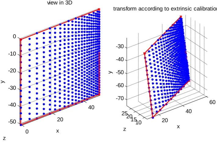
The distances between the camera and different regions of the board were not identical, and because of this, the structured light reconstructed point cloud had a higher density of points in regions closer to the camera than regions further away. The effect can be recreated by a perspective transformation and the concept is explained in Figure 3.6. Imagine a camera capturing the image of a square positioned on a steep angle to the optical axis of the camera (Figure 3.6, left), while the image appears to have uniform resolution (shown as blue dots), the distribution of image pixels across the plane is in fact uneven and this can be seen by transforming the viewing direction to align with the normal of the plane (Figure 3.6, right).

Figure 3.6. Left, image plane of a camera looking from a steep angle, at a square region bounded by the red lines, the blue dots represent camera pixels. Right, the same setup but now from the square board's perspective. This is an exaggerated example, in actual measurements, the camera look angle was never as steep as what is shown here.

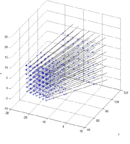
The location of the pixels in physical coordinates could then be calculated using the perspective transformation, and based on the dimension of the square (Figure 3.6 right and Figure 3.7 left). From the extrinsic calibration results, the point cloud can be transformed (see Figure 3.7 right) by the exact same method as the transformation of the four fiducial corners in the previous section. The transformed point cloud is stored in an n by 3 array in which the nth row represents the 3D coordinate of the same pixel on the image, as the nth row structured light reconstructed point cloud (see Figure 3.8).

10 20 30 40 50 10 20 30 40 50 60 70 80 camera perspective

pixel coordinate x

p ix e l c o o rd in a te y

0 20 40

47

Figure 3.7. Recovering 3D coordinates for every image pixel within the square region using extrinsic calibration results.

Figure 3.8. Every camera pixel within the red region (see Figure 3.6 Left) has its 3D coordinates calculated twice, one using structured light (cyan) the other using extrinsic calibration (blue). The point clouds shown here were generated for explanation purposes. 20 40 60 10 15 20 25 -70 -60 -50 -40 -30 x

transform according to extrinsic calibration

z y 0 20 40 -50 -40 -30 -20 -10 0

view in 3D

48

3.2.2. Results

Effects of triangulation angle

The structured light reconstructions of the plane presented in section 3.1 were re-analyzed using the described method. Offsets between the two types of measurement were calculated for each encoded pixel. For each pixel, the triangulation angle, which refers to the angle between a projector plane and an intersecting camera ray, was calculated and compared to the error at that pixel. They were observed to be inversely correlated in two of the three orientations (see Figure 3.9), with linear correlation coefficients of -0.78 (magenta) and -0.61 (red), and statistically independent in the third orientation with a correlation coefficient of 0.21 (blue).

Figure 3.9. Relationship between triangulation angle and error.

An inverse correlation between triangulation angle and error is plausible. Consider a simplified triangulation problem in a 2D projector and camera system, let the angle between the projector ray and the projector optical axis carry an offset of -0.5o (assume this came from inaccurate projector calibration), and the camera ray has a negligible error. If the true triangulation angle was 22o, and the true point of

18 19 20 21 22 23 24 25 26 27 28 0

0.5 1 1.5 2 2.5 3 3.5 4

angle between camera ray and projector plane

%

o

ff

s

e

49

intersection was 1m from the projector (l = 1, see Figure 3.10) the offset of -0.5o will result in an error of 2.4cm over the distance of 1m, if the true triangulation angle was 26o, the same offset in angle would now generate a 2.0cm error, if the triangulation angle was increased further to 44o, the error would be lowered to 1.3cm. The general expression for the expected distance offset, d, is given by the sine rule:

𝑑 sin 𝐷=

s sin 𝜃=

𝑙

sin 𝜑 (3.1)

where l is the length of the true projector ray vector l, 𝜃 is the true angle of triangulation, s is the length of projector ray vector s found by calibration, 𝜑 is the triangulation angle measured in calibration, and D is the angle offset. This

explanation could not account for the large magnitude of error observed for the given range of triangulation angles, it never the less showed the accuracy of a structured light system is susceptible to the positions and view angles of the camera and projector with respect to each other.

Figure 3.10. Error in the triangulation result (d) caused by a discrepancy between the true direction (green) and the calibration result (red) of a projector ray.

Accuracy across the projection field

50

(see Figure 3.11) with correlation coefficients of: -0.8575 (blue), -0.9153 (red), and -0.9401 (magenta). For this particular projector and camera setup, the structured light reconstructions were less accurate in regions encoded by the left of the projection field where the system tended to overestimate the distance from the camera. The accuracy of the reconstruction improves linearly towards the centre of the projection field. The right part of the projection (columns 650-1024) was not used due to the location of the board during encoding.

Figure 3.11. Relationship between the encoding plane indices and error.

Angle between projector planes

The angles of separation between each pair of neighbouring projection planes were calculated. This was done to help visualize the orientations of the projector columns in space, which was used as a check for the validity of the projector calibration result. The angle profile across the width of the projection field took the shape of a

parabola (see Figure 3.12), it peaked at 0.0361o around column 489 of the projection, and fell to around 0.0316o, and 0.0309o towards the left and right sides respectively. The varying separation angle of the projecting columns was not unexpected, digital projectors were designed for use on a flat screen , the distance light traverses from

200 250 300 350 400 450 500 550 600 650 0

0.5 1 1.5 2 2.5

encoding projector plane index

%

o

ff

s

e