Unsupervised Segmentation Method of Multicomponent Images based on Fuzzy Connectivity Analysis in the Multidimensional Histograms

Unsupervised Segmentation Method of Multicomponent

Images Based on Fuzzy Connectivity Analysis in the

Multidimensional Histograms

Sié Ouattara1, Georges Laussane Loum1, Alain Clément2

1_{Laboratoire d’Instrumentation, d’Image et de Spectroscopie (L2IS), Institut National Polytechnique Félix}

Houphouët-Boigny (INPHB), Yamoussoukro, Côte d’Ivoire

2_{Laboratoire d’Ingénierie des Systèmes Automatisés (LISA), Institut Universitaire de Technologie,}

Angers Cedex, France E-mail: [email protected]

Received January 20, 2011; revised February 9, 2011; accepted February 15, 2011

Abstract

Image segmentation denotes a process for partitioning an image into distinct regions, it plays an important role in interpretation and decision making. A large variety of segmentation methods has been developed; among them, multidimensional histogram methods have been investigated but their implementation stays difficult due to the big size of histograms. We present an original method for segmenting n-D (where n is the number of components in image) images or multidimensional images in an unsupervised way using a fuzzy neighbourhood model. It is based on the hierarchical analysis of full n-D compact histograms integrating a fuzzy connected components labelling algorithm that we have realized in this work. Each peak of the histo- gram constitutes a class kernel, as soon as it encloses a number of pixels greater than or equal to a secondary arbitrary threshold knowing that a first threshold was set to define the degree of binary fuzzy similarity be- tween pixels. The use of a lossless compact n-D histogram allows a drastic reduction of the memory space necessary for coding it. As a consequence, the segmentation can be achieved without reducing the colors population of images in the classification step. It is shown that using n-D compact histograms, instead of 1-D and 2-D ones, leads to better segmentation results. Various images were segmented; the evaluation of the quality of segmentation in supervised and unsupervised of segmentation method proposed compare to the classification method k-means gives better results. It thus highlights the relevance of our approach, which can be used for solving many problems of segmentation.

Keywords:Multicomponent Images, Unsupervised Segmentation, n-D Histogram, Fuzzy Connected

Components Labelling, n-D Compact Histogram, Evaluation of Segmentation Quality

1. Introduction

In many fields such as medicine, food, robotics, security systems, etc, the acquisition and the analysis of images are essential processes for taking decisions [1-4], as it is often difficult to perform them manually, it is necessary to automate certain tasks by computing. Thus in this pa- per, we present, a new vectorial segmentation method based more particularly on the full n-D compact histo- grams by a fuzzy connexity analysis.

Segmentation is an important step in image processing and automatic pattern recognition processes based on image analysis as subsequent extracted data are highly

A few years ago, we have proposed a new way of cod- ing the nD histograms, leading to the so-called compact histogram [6], in which only the occupied cells of the classical histogram are memorised. This reduces the memory space required drastically: it is lowered to a value of 500 ko for a 256  256 image with color com- ponents coded on 8 bits, without any loss of color infor- mation, it shows its efficiency in previous articles [7,8].

Using histograms for classifying colour pixels can be achieved through four different strategies.

The first strategy proceeds in a marginal way. Each component of the histogram is examined separately [9,10]. The method is easy to implement, but it does not take into account the correlation between colorimetric components.

In the second strategy, each colorimetric component is requantized on q bits (q < 8) in order to reduce the histo- gram size [11]. The method is efficient, but it makes an a priori color classification.

The third strategy that many authors have developed proceeds by projection of the 3-D histogram on two of the three colorimetric axes. W have developped this strategy in a previous paper [12] and used also in other articles such as [13-15]; The histogram, with populations requantized on 256 levels, is considered as a gray level image and processed by a watershed algorithm. The cor- relation between components is partially taken into ac- count, but the requantization of the populations alters the true histogram, and the projection can result in ignoring some significant classes.

Here we propose a fourth strategy. It is fully vectorial, which is allowed by the use of the compact n-D histo- gram. Its principle consists in finding the peaks of classic multidimensional histogram using the compact multidi- mensional histogram by the consideration of a model of fuzzy neighbourhood. The kernels of the built classes correspond to the peaks retained using the algorithm for labelling connected components with binary fuzzy neighbourhood that we realized in this work, it accepts two input parameters which are the degree of fuzzy connectedness expressing the similarity between the vector points of the compact n-D histogram and a population threshold limiting the class size. The choice of the fuzzy connectedness here is justified by the difficulty of defining a net similarity between the vector points attribute or “colors” of the pixels of the image [16,17]. This leads to different results of segmentation of the same number of classes for different values of pairs of thresholds. Assessing the quality of segmentation can choose the most relevant segmentation. The results of our multidimensional segmentation method are compared to those of the method of classification K-means [13,18, 19] in order to evidence the performance of our approach

using supervised and unsupervised [20-23] evaluation methods of the segmentation quality.

2. A Fast and Compact Multidimensional

Histogram

We consider multicomponent images (for example mul- tispectral images) with n components Ii





1 to n, each Ii has a tonal resolution of Q possible values

and each pixel of spatial coordinate





value among the Q possibilities. A n-dimensional histo- gram of such an image would comprise Qn _{cells. For an}

image with N pixels of resolution, only at most N of these Qn _{cells can be occupied, meaning, as n grows,}

most of the cells of the n-dimensional histogram are in fact empty. For example, for a commun 512 × 512 RGB color image with n = 3 and Q = 256, there are Qn _{= 256}3_≈ 16 × 106 _{colorimetric cells of n-tuples with at most only} 3N = 5122 _{= 262144 of them which can be occupied. The} idea of a compact representation of the n-dimensional histogram [6], where only those cells that are occupied are coded. The n-dimensional histogram is coded as a linear array where the entries are the n-tuples (the colors) present in the image and arranged in lexicographic order of their components (I1, I2, , In). To each entry (in number ≤ N) is associated the number of pixels in the image having this n-value (this color). An example of this compact representation of the n-dimensional histo- gram is shown in Table 1.

The practical calculation of such a compact histogram starts with the lexicographic ordering of the N n-tuples corresponding to the N pixels of the image. The result is a linear array of the N ordered n-tuples with their popula- tion. With a dichotomic quick sort algorithm to realize the lexicographic ordering, the whole process of calcu- lating the compact multidimensional histogram can be achieved with an average complexity of O(N logN), in- dependent of the dimension n. Therefore, both compact

Table 1. An example of compact coding of the 3-dimen-

sional histogram of an RGB color image with Q = 256. The

entries of the linear array are the components (I1, I2, I3) =

(R, G, B) arranged in lexicographic order, for each color present in the image, and associated to the population of pixels having this color.

R G B population

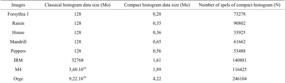
representation and its fast calculation are afforded by the process for the multidimensional histogram. For example, for a 9-component 838 × 762 satellite image with Q = 256, the compact histogram was calculated in about 5 s on a standard 1 GHz clock desktop computer, with a coding volume of 1.89 Moctets, while the classic histo- gram would take 3.60 × 1016 _{Moctets completely un-} manageable by today’s computers.

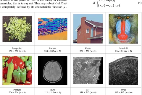
The advantages of the compact multidimensional ap- plied to multicomponent images (see Figure 1) are shown in Table 2.

3. Fuzzy Connected Components Labeling of

Compact Histogram

3.1. Formalism of Fuzzy Logic and Concept of Fuzzy Neighbourhood

We present here some aspects of the theory of fuzzy logic, fundamental to understanding the algorithm of Fuzzy Connected Component Labeling (FCCL) compact multidimensional histograms, developed in following sections. The reader will find a complete overview in [24].

X denote the universe of reference, consisting of elements x, and place us first in the theory of classical ensembles, that is to say net. Then any subset A of X net is completely defined by its characteristic function µA,

defined on the set {0,1} score, by:

 

ssi x A x

 _{ } 

 (1)

If the set score is now the continuum [0,1], A becomes a fuzzy subset of X, and µA is its membership function.

The subset A is then defined by:

 





A _x  x _ x X (2)

An α-cut of A is the net subset of items with a membership degree to A greater than or equal to α. It is noted Cα(A):

 



 



C_ A  x X  x  (3)

The concept of fuzzy relation is a generalization with the fuzzy domain of the concept of equivalence relation defined in the net case. A fuzzy relation can be measured by a scalar in the interval [0,1], the degree to which a logical proposal is verified. With a fuzzy relation R is associated membership function, denoted by µR. Let X

and Y be two universes of reference, the respective elements x and y. A fuzzy relation between the elements of these two worlds is formally defined as:

 

 

 

0,1 :

, R ,

X Y R

x y  x y

   



  (4)

Forsythia 1 652 × 578 (n = 3)

Raison 384 × 287 (n = 3)

House 256 × 256 (n = 3)

Mandrill 256 × 256 (n = 3)

Peppers 256 × 256 (n = 3)

IRM 512 × 512 (n = 4)

M4 838 × 762 (n = 9)

Orge 512 × 512 (n = 10)

Table 2. Comparative table of volumes of the classical and compact histograms of the images of Figure 1.

Images Classical histogram data size (Mo) Compact histogram data size (Mo) Number of spels of compact histogram (N)

Forsythia 1 128 0,28 73278

Raisin 128 0,35 90802

House 128 0,36 33925

Mandrill 128 0,65 61662

Peppers 128 0,56 53488

IRM 32768 1,61 140881

M4 3,60.1016 _{1,89 116425}

Orge 9,22.1018 _{4,22 246104}

When X=Y, the fuzzy relation is known as binary. In one of the following sections will be built a fuzzy connected component labeling of compact multidimen- sional histogram (it is him which plays the role of universe of reference X). The labelling will use a binary fuzzy relation, which we call fuzzy similarity, assessing the degree of similarity between two spells x and y of compact histogram multidimensional. The membership function of this relationship will be expressed as:

 

 

 

si d x y M

d x y x y



 _

   

 

(5)

This model of fuzzy neighborhood is used in many studies [25,26]. In our case, the threshold M is set at 7 which is the maximum distance allowed so that two spells resembles itself, and the distance d considered will be that of Chebychev or again call Queen-wise distance, given by the following equation:

 

, maxn i i

i

d x y x y



  (6)

3.2. Classical Connected Components Labelling

We have recently achieved [8] the connected compo- nents labelling (CCL) of n-D compact histograms. It consists in sweeping all the n-tuples present in the com- pact histogram, in order to gather, under the same label, the n-uplets which are neighboring in the n-D colorimet- ric space.

Since the n-uplets are ordered in lexicographical order inside the compact histogram, labelling a n-tuple is achieved by sweeping only the (3n_{-1)/2 n-tuples con-}

nected neighbours preceding it. For example, Table 3 shows the four doublets of (i,j) to be swept for labelling the doublet (i,j) in the case of 2-D compact histograms.

The CCL is applied to the full n-D compact histo- grams of five multicomponent images (see Figure 1)

Table 3. Connected neighbours to be swept for CCL of

doublet (i, j) in the case of a 2-D compact histogram (col-

orimetric axes I and J).

Plan I Plan J

0 0 … … i-1 j-1 i-1 j i-1 J+1 … … i j-1

i j

… …

2Q_{-1 2}Q_-1

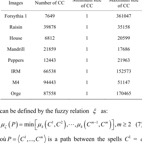
taken on the web site of gdr-isis. Table 4 shows the number of connected components (CC) of their histo- grams and, the minimum and maximum size of CC are expressed as number of pixels compared to the size of the images.

3.3. Principle of Fuzzy Connected Components Labelling

Table 4. Statistics in related connected components of the images of Figure 1.

Images Number of CC Minimum size _{of CC} Maximum size _{of CC}

Forsythia 1 7649 1 361047

Raisin 39878 1 35158

House 6812 1 20599

Mandrill 21859 1 17686

Peppers 12443 1 21963

IRM 66538 1 152573

M4 94443 1 51147

Orge 87558 1 170465

can be defined by the fuzzy relation  as:

 









k k

P C C C C m



 _{ }   _{ }

   (7)

où_{P C}1_,...,Cm _{is a path between the spells C}1 _{= c} and Cm _{= d. As several paths may exist between spell c} and d, the overall cost of the paths is defined as the maximum value of all path costs calculated on the set of paths. The overall cost of paths between two related spell c and d in the histogram can then be defined by the fuzzy relation  as:

 

 

P P

 

 

  

 _{ } (8)

The fuzzy relation  is an equivalence relation. The definition of a  -neighborhood between two spels re- quires to fix a minimum threshold of similarity which we denote  . This threshold being fixed, find the prede- cessors of a spel c returns searching its neighbors of a minimum cost  i.e the spels of the net set  -cut of the fuzzy relation  .

Let d be an element of the set of predecessors of c in the compact histogram Hc.

 



 



Predecessors c  dHc_ c d  (9)

The principle of the CCLF is similar to that of the CCL, with for only difference the research of predeces- sors of a spel in compact histogram as shown by Equa- tion (9). In practice we will vary the value of  to study its influence on the number of connected compo- nents. Two values bring back to us to particular cases:

 when  1, the spels of the compact histogram are considered each one as a connected component, so the number of connected components equals the number of spels;

 when  0.5 the CCLF corresponds to the CCL.

3.4. Our Algorithm of Fuzzy Connected Components Labelling

The proposed algorithm integrates the search of fuzzy predecessors, their number being limited by the fixation of overall cost . The algorithm returns as output the vector E containing the labels of spels as they appear in the compact histogram, and the number of connected components (NberCc) of the histogram.

[ , ] ( , )

function E NberCc FCCL Hc //Hc: compact n-D histogram //E: table of spels label

//NberCc: number of connected components //Tequiv: management table of equivalences Label

//taille: function that returns the number of rows in a table

//elimineRedondance: removes redundant elements of an array

//max: function that returns the maximum of an array

//min: function that returns the minimum of a ta-ble

N = taille(Hc) //number of spels of n-D compact histogram

E(1) = 1 //label of the first spel of Hc to 1 Tequiv(1) = 1 //equivalence label 1 to 1 For i = 2: N

P = Hc(i,:) //current spel labeling j = i -1

IndexPred = Ø





1

1

d   _

For j =1: i-1

While (Hc j( ,1)Hc i( ,1)d1) c = Hc(j,:)

If (k( , )c d  )

IndexPred = [Index-Pred; j]

EndIf EndWhile EndFor

If (taille(IndexPred)  0)

Etiq = E(IndexPred)//returns the labels of the predecessors

Etiq = elimineRedondance(Etiq) EndIf

If (taille(Etiq) == 0) E(i) =1 + max(E) Tequiv(E(i)) = E(i) ElseIf (taille(Etiq) ==1)

E(i) = min(Etiq)

Tequiv(E(IndexPred)) = E(i) EndIf

EndFor For i = 2:N

E(i) = Tequiv(E(i)) //global update of labels EndFor

3.5. Example of Results

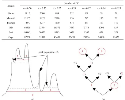
The FCCL algorithm is applied on the compact n-D his- tograms of multicomponent images in Figure 1. Table 5 illustrates the results for different values of  . It shows that when the degree of similarity  decrease, the number of connected components (CC) decrease.

4. Fuzzy Vectorial Classification of Tuples

4.1. Principle

The classification of colours is carried out in two steps:

the learning step and the decision step.

The learning step is a hierarchical decomposition of populations in the compact n-D histogram. For each level of population pn, peaks Pi are identified by the FCCL

algorithm for a given value of α, which retains the con- nected components whose populations are greater than or equal to pn. Each peak is then iteratively decomposed

into narrower peaks, beginning from population 0. A peak is labelled as significant if it represents a population greater than or equal to a threshold S (expressed in per- cent of the total population in the histogram). The pro- cedure is illustrated in part a of Figure 2 (drawn in one dimension for clarity). We shall name kernels Ki the

peaks corresponding to circled leaves in part b of Figure 2. In other words, kernels are significant peaks (part a of Figure 2) without descendants in the hierarchical de- composition tree (part b of Figure 2) (e.g., Figure 2 shows five significant peaks Pi (i = 0 to 4) and three

kernels Ki (i = 2, 3, 4)). The number of classes Nc is

taken equal to the number of kernels (the class corre- sponding to kernel Ki is noted Ci). Therefore Nc depends

Table 5. Statistics in related fuzzy connected components of the images of Figure 1.

Images Number of CC

α= 0.50 α= 0.33 α= 0.25 α= 0.20 α= 0.17 α = 0.14 α = 0.125 House 6812 2000 684 252 108 59 28

Mandrill 21859 5939 2016 736 279 106 57

Peppers 12443 3277 1130 514 261 153 110

IRM 66538 33594 16572 7687 3718 1704 837

M4 94443 30373 8583 3020 1307 678 379

Orge 87558 55312 43431 35493 29236 24808 21423

(a) (b)

Figure 2. An example of hierarchical decomposition with α = 0.5. The circled leaves (part (b)) correspond to significant peaks

as obtained at the end of the iterative decomposition (solid lines in part (a)), whereas leaves marked < S (part (b)) correspond

on the threshold S, i.e. on the precision the image colors are analyzed with and the value of α the degree of simi- larity between the spels.

In the decision step, the mass center µ(Ki) of each ker-

nel Ki is calculated in the feature multidimensional space.

Let us denote by ß the color corresponding to the point of coordinates (g1, g2, , gn) in the feature space. Two

cases appear: if (g1, g2, , gn) belongs to Ki, color ß is

attributed to class Ci; if not, let us denote by Pk the peak

which belong to (g1, g2, , gn); color ß is attributed to

class Ci corresponding to kernel Ki, son of Pk, such that

d[µ(Ki), (g1, g2, , gn)] is minimum, where d[y, z] is the

Euclidean distance between y and z.

We give a name of this method that we call Hierar- chieFuzzy_nD.

4.2. Results of Segmentation

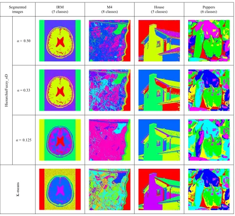
The following figure denote Figure 3 shows an example of segmented images by HierarchieFuzzy_nD and K-means methods.

5. Methods for Assessing the Quality of

Segmentation

Image segmentation is a fundamental process in image and video analysis. Several approaches have been put forward in the literature [22,29]. We have the region, contour and texture approaches, but this work interests the region approach. It is often used to partition an image into separate regions, which ideally correspond to different

Segmented

images (5 classes) IRM (8 classes) M4 (5 classes) House (6 classes) Peppers

Hierar

chieFuzzy_

n

D

α = 0.50

α= 0.33

α = 0.125

K-means

real-world objects.

Many segmentation methods exist in literature, but it is difficult to evaluate the efficiency and to make an ob- jective comparison of different segmentation methods. This general problem has been addressed for the evalua- tion of a segmentation result [20]. There are two main approaches:

 There are supervised evaluation criteria based on the computation of a dissimilarity measure between a segmentation result and ground truth. Baddeley’s distance [30], Vinet’s measure [31], or Hausdorff’s measure [32] are examples of supervised evalua- tion criteria. In practice the ground truth of natural images is a segmentation results manually made by experts.

 There are unsupervised evaluation criteria that en- able the quantification of the quality of a segmen- tation result without any a priori knowledge. These criteria generally compute statistical measures such as standard deviation or the disparity of each re- gion or class in the segmentation result [33-36]. Currently in practice, no evaluation criterion appears to be satisfactory in all cases [22]. However, we choose here the best criterion for each type of evaluation, i.e. Vinet measure for supervised evaluation and Zeboudj measure in unsupervised case [22].

One potential benefit of supervised methods over un- supervised methods is that the direct comparison be- tween a segmented image and a reference image is be- lieved to provide a finer resolution of evaluation, and as such, discrepancy methods are commonly used for ob- jective evaluation. However, manually generating a ref- erence image is a difficult, subjective, and time-con- suming task [20].

5.1. Vinet Measure

The Vinet’s measure [31] that is a supervised criterion which corresponds to the correct classification rate is used as reference for the analysis of the synthetic images. In this case, the ground truth is available. This criterion is often used to compare a segmentation result IR with

a ground truth I_RRef in the literature. We compute the

following superposition table:









  Re

,

, f ,

Ref

R _R i j

i j

T I I 



Where





i j

card R R is the number of pixels result- ing from the intersection of regions Ri and Rj in the

ground truth. The best match between Ri and Ref j

R is

one that maximizes T I I





a dissimilarity measure, it is computed as follows:





 

_{ }





Ref

R i j

R Ref

R

Card I Card R R

Vinet I I

Card I

 

 (11)

This criterion is often used to compute correct classi- fication rate of the segmentation result of a synthetic image.

5.2. Zeboudj Criterion

Zeboudj [35] proposed a measure based on the combined principles of maximum interregions disparity and mini- mal intraregion disparity measured on a pixel neighbor- hood. Zeboudj’s criterion is defined by:

 

   

_{ }

R

Card R C R

Zeboudj I

Card I







Where C R

 

 

This criterion is suitable for evaluating segmentation of homogeneous and little texture images.

6. Results and Discussion

The tests were performed on many multicomponent im-ages. A synthetic illustration of the evaluation of our method of segmentation is applied to images of Figure 1 with a variation in the number of classes per image to be segmented.

Indexed Table 6(a) to (f) contains the results of the unsupervised evaluation applied to different images of which we doesn’t ground-truth. However Table 7 illus- trates the results of the supervised evaluation obtained from 24 images of forsythia and 1 grape image of which we have their ground-truth.

The relevance of our method of segmentation is made with respect to k-means known in the world of image processing because of its simplicity and its performance.

The Table 7 shows that in supervised evaluation, the fuzzy multidimensional hierarchical method of segmen- tation HierarchieFuzzy_nD outperforms k-means for each image. This is explained by its ability to detect col- orimetrically or spectrally similar classes.

The indexed Table 6 by (a) to (e) evaluates in a syn- thetic way HierarchieFuzzy_nD comparing it systematic- cally to k-means and by putting forward the evaluation of HierarchieFuzzy_nD in the case of the classical connex- ity between spels i.e for α = 0,5. Thus can be drawn the following conclusions:

the spectral data by solving the problem of colori- metric or spectral similarity between spels of the multidimensional histogram.

 While limiting oneself to alpha = 0,5 correspond- ing to the traditional connexity, we note that for the images M4 and Orge of which the number of spec- tral plans is high, that HierarchieFuzzy_nD is sys- tematically considered to be less powerful than k-means. This lower performance is a consequence

of the phenomenon of over-segmentation justified by the Table 4 which shows the widespread prob- lem of the spels of the nD histograms in a multidi- mensional space when n is large, hence the interest of the introduction of fuzzy connectedness between spels characterized by the parameter α, highlight- ing the relevance of HierarchieFuzzy_nD. The major drawback of this last is to be costly in com- puting time.

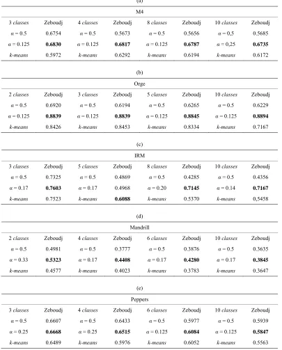
Table 6. Unsupervised evaluation of multicomponent images segmentation; in red, segmentations considered to be the best.

(a) M4

3 classes Zeboudj 4 classes Zeboudj 8 classes Zeboudj 10 classes Zeboudj

α= 0.5 0.6754 α= 0.5 0.5673 α= 0.5 0.5656 α= 0,5 0.5685

α= 0.125 0.6830 α= 0.125 0.6817 α= 0.125 0.6787 α= 0,25 0.6735

k-means 0.5972 k-means 0.6292 k-means 0.6194 k-means 0.6172

(b) Orge

2 classes Zeboudj 3 classes Zeboudj 5 classes Zeboudj 10 classes Zeboudj

α= 0.5 0.6920 α= 0.5 0.6194 α= 0.5 0.6265 α= 0.5 0.6229

α= 0.125 0.8839 α= 0.125 0.8839 α= 0.125 0.8845 α= 0.125 0.8894

k-means 0.8426 k-means 0.8453 k-means 0.8334 k-means 0.7167

(c) IRM

3 classes Zeboudj 5 classes Zeboudj 8 classes Zeboudj 10 classes Zeboudj

α= 0.5 0.7325 α= 0.5 0.4869 α= 0.5 0.4285 α= 0.5 0.4356

α= 0.17 0.7603 α= 0.17 0.4968 α= 0.20 0.7145 α= 0.14 0.7167

k-means 0.7523 k-means 0.6088 k-means 0.5370 k-means 0,5458

(d) Mandrill

2 classes Zeboudj 4 classes Zeboudj 6 classes Zeboudj 10 classes Zeboudj

α= 0.5 0.4981 α = 0.5 0.3777 α= 0.5 0.3876 α= 0.5 0.3635

α = 0.33 0.5323 α = 0.17 0.4408 α = 0.17 0.4280 α= 0.17 0.3845

k-means 0.4577 k-means 0.4023 k-means 0.3783 k-means 0.3647

(e) Peppers

3 classes Zeboudj 4 classes Zeboudj 6 classes Zeboudj 10 classes Zeboudj

α= 0.5 0.6607 α= 0.5 0.6433 α= 0.5 0.5977 α= 0.5 0.5939

α= 0.25 0.6668 α= 0.25 0.6515 α= 0.125 0.6084 α= 0.125 0.5847

k-means 0.6489 k-means 0.5976 k-means 0.6052 k-means 0.5563

Table 7. Supervised evaluation of real images segmentation; in red, segmentations considered to be the best.

HierarchieFuzzy_nD K-means Vinet (%)

Forsythia (2classes)

Seg_Img01 5.78 8.43

Seg_Img02 6.11 10.22

Seg_Img03 6.04 8.98

Seg_Img04 5.34 11.06

Seg_Img05 5.46 9.84

Seg_Img06 4.34 9.36

Seg_Img07 8.26 14.06

Seg_Img08 5.46 10.43

Seg_Img09 4.69 10.66

Seg_Img10 4.85 10.35

Seg_Img11 5.58 12.21

Seg_Img12 3.65 6.93

Seg_Img13 3.57 6.88

Seg_Img14 4.00 7.07

Seg_Img15 5.27 12.08

Seg_Img16 5.58 11.71

Seg_Img17 4.52 8.05

Seg_Img18 4.21 13.22

Seg_Img19 4.18 8.57

Seg_Img20 4.88 8.44

Seg_Img21 6.87 18.99

Seg_Img22 5.04 9.42

Seg_Img23 5.53 8.52

Seg_Img24 4.19 9.44

Seg_Raisin

(3 classes) 5.76 5.96

7. Conclusion

This work is a contribution to the classification by the analysis of multidimensional histograms. It proposes a vectorial strategy to segment color or multicomponent images and provides the tools necessary for its imple- mentation. This work is accompanied by a more general reflexion on the principle of classification in a multidi- mensional space in connection with the evaluation me-thods of segmentation.

We have liberated the large volume of multidimen- sional histograms using the nD compact histogram for which we have proposed a fuzzy algorithm for labeling connected components. This algorithm allowed us to

develop an unsupervised and nonparametric method by vectorial classification of multidimensional histograms. We made a solution to the problem of over-segmentation generated by the appearance diffuse of multidimensional histograms and evaluated our segmentation results.

We chose to approach the Classification by analyzing histograms nonparametrically with emphasis on algo- rithmic and geometric approaches comparatively to sta- tistical approaches. We justify this choice by the need first there was to provide solutions to the problem of dealing vectorially histograms of multicomponent im- ages because of their size. The tools that we have devel- oped, allowed us to better understand the mechanism of classification in a multidimensional space and to open channels to predict outcomes.

In Perspective, this work can be directly exploited to define new vectorial methods or strategies for the analy- sis of multidimensional histograms and their classifica- tion. The algorithms developed here can be used to serve statistical or spatio-colorimetric approaches for the seg- mentation of color and multicomponent images.

8. References

[1] R. Furferi, “Colour Classification Method for Recycled Melange Fabrics,” Journal of Applied Sciences, Vol. 11, No. 2, 2011, pp. 236-246. doi:10.3923/jas.2011.236.246 [2] W. Yanqing, C. Deyun, S. Chaoxia and W. Peidong,

“Vi-sion-Based Road Detection by Monte Carlo Method,” Information Technology Journal, Vol. 9, 2010, pp. 481- 487.

[3] P. Vijayaprasad, M. N. Sulaiman, N. Mustapha and R. W. O. K. Rahmat, “Partial Fingerprint Recognition Using Support Vector Machine,” Information Technology Jour- nal, Vol. 9, No. 4, 2010, pp. 844-848.

doi:10.3923/itj.2010.844.848

[4] L. Lixiong, W. Yuwei and W. Yuanquan, “A Novel Me-thod for Segmentation of the Cardiac MR Images using Generalized DDGVF Snake Models with Shape Priors,” Information Technology Journal, Vol. 8, No. 4, 2009, pp. 486-494. doi:10.3923/itj.2009.486.494

[5] R. Gonzalez and O. Wintz, “Digital Image Processing,” 3rd Edition, Addison-Wesley Publishing Co., Massachu- setts, 1991.

[6] A. Clement and B. Vigouroux, “A Compact Histogram for the Analysis of Multicomponent Images,” Proceed-ings of 18th Conference GRETSI on Signal Processing, Vol. 1, 2001, pp. 305-307.

[7] S. Ouattara, A. Clément and F. Chapeau-Blondeau, “Fast Computation of Entropies and Mutual Information for Multispectral Images,” Proceeding of 4th International Conference on Informatics in Control, Automation and Robotics, Angers, Vol. 1, May 2007, pp. 195-199. [8] S. Ouattara and A. Clement, “Labelling of Compact Mul-

the Image Processing, Troyes, September 2007, pp. 85-88. [9] L. Busin, N. Vandenbroucke, L. Macaire and J.-G.

Post-aire, “Color Space Selection for Unsupervised Color Im-age Segmentation by Histogram Multithresholding,” Proceedings of IEEE International Conference on Image Processing (ICIP’04), 2004, pp. 203-206.

[10] J. Hemming and T. Rath, “Computer-Vision-Based Weed Identification under Field Conditions Using Controlled Lighting,” Journal of Agricultural Engineering Research, Vol. 78, No. 3, 2001, pp. 233-243.

doi:10.1006/jaer.2000.0639

[11] G. Xuan and P. Fisher, “Maximum Likelihood Clustering Method Based on Color Features,” Proceedings of the First International Conference on Color in Graphics and Image, Saint-Etienne, 2007, pp. 191-194.

[12] A. Clement and B. Vigouroux, “Unsupervised Segmen- tation of Scenes Containing Vegetation (Forsythia) and Soil by Hierarchical Analysis of Bidimensional Histo-grams,” Pattern Recognition Letters, Vol. 24, No. 12, August 2003, pp. 1951-1957.

doi:10.1016/S0167-8655(03)00034-5

[13] W.-Y. Wei, Z.-M. Li, G.-C. Zhang and G.-Q. Zhang, “Novel Color Microscopic Image Segmentation with Si-multaneous Uneven Illumination Estimation Based on PCA,” Information Technology Journal, Vol. 9, No. 8, 2010, pp. 1682-1685. doi:10.3923/itj.2010.1682.1685 [14] O. Lezoray and C. Charrier, “Color Image Segmentation

using Morphological Clustering and Fusion with Auto-matic Scale Selection,” Pattern Recognition Letters, Vol. 30, No. 4, March 2009, pp. 397-406.

doi:10.1016/j.patrec.2008.11.005

[15] O. Lezoray, “Unsupervised 2D Multiband Histogram Clustering and Region for Color Image Segmentation,” Proceedings of the 3rd IEEE International Symposium on Signal Processing and Information Technology, 2003, pp. 267-270.

[16] C. G. Looney, “Fuzzy Connectivity Clustering with Radial Basis Kernel Functions,” Fuzzy Sets and Systems, Vol. 160, No. 13, 2009, pp. 1868-1885.

doi:10.1016/j.fss.2008.12.010

[17] O. Nempont, J. Atif, E. Angelini and I. Bloch, “A New Fuzzy Connectivity Measure for Fuzzy Sets: And Asso-ciated Fuzzy Attribute Openings,” Journal of Mathemat-ical Imaging and Vision, Vol. 34, No. 2, 2009, pp. 107-136. doi:10.1007/s10851-009-0136-3

[18] D. Al-Bashish, M. Braik and S. Bani-Ahmad, “Detection and Classification of Leaf Diseases Using K-Means- Based Segmentation and Neural-Networks-Based Classi-fication,” Information Technology Journal, Vol. 10, No. 2, 2011, pp. 267-275. doi:10.3923/itj.2011.267.275 [19] S. Dehuri, C. Mohapatra, A. Ghosh and R. Mall, “A

comparative Study of Clustering Algorithms,” Informa-tion Technology Journal, Vol. 5, 2006, pp. 551-559. doi:10.3923/itj.2006.551.559

[20] H. Zhang, J. E. Fritts and S. A. Goldman, “Image Seg-mentation Evaluation: A Survey of Unsupervised Me-thods,” Computer Vision and Image Understanding, Vol. 110, No. 2, 2008, 260-280.

doi:10.1016/j.cviu.2007.08.003

[21] O. Kubassova, M. Boesen and H. Bliddal, “General Framework for Unsupervised Evaluation of Quality of Segmentation Results,” 15th IEEE International Confe- rence on Image Processing (ICIP’08), 2008, pp. 3036- 3039.

[22] S. Chabrier, B. Emile, C. Rosenberger and H. Laurent, “Unsupervised Performance Evaluation of Image Segmen- tation,” EURASIP Journal on Applied Signal Processing, 2006, pp. 1-12. doi:10.1155/ASP/2006/96306

[23] C. P. Juan, E. S. David and F. R. Francisco, “Image Seg-mentation Based on Merging of Sub-Optimal Segmen- tations,” Pattern Recognition Letters, Vol. 27, No. 10, 2006, pp. 1105-1116.

[24] D. Dubois and H. Prade, “Fuzzy Sets and Systems — Theory and Applications,” Academic Press, New York, 1980.

[25] I. Bloch, “Fuzzy Spatial Relationship for Image Processing and Interpretation: A Review,” Image and Vi-sion Computing,” Vol. 23, No. 2, February 2005, pp. 89-110. doi:10.1016/j.imavis.2004.06.013

[26] C. Demko and E. Zahzah, “Image Understanding Using Fuzzy Isomorphism of Fuzzy Structures,” Proceedings of International Joint Conference of the Fourth IEEE In-ternational Conference on Fuzzy Systems and the Second International Fuzzy Engineering Symposium, Yokohama, Vol. 3, 1995, pp. 1665-1672.

[27] B. M. Carvalho, G. T. Herman and T. Y. Kong, “Simul-taneous Fuzzy Segmentation of Multiple Objects,” Dis-crete Applied Mathematics, Vol. 151, No. 1-3, 2005, pp. 55-77. doi:10.1016/j.dam.2005.02.031

[28] P. K. Saha, J. K. Udupa and D. Odhner, “Scale-Based Fuzzy Connected Image Segmentation: Theory, Algo-rithms, and Validation,” Computer Vision and Image Understanding, Vol. 77, No. 2, 2000, pp. 145-174. doi:10.1006/cviu.1999.0813

[29] J. Freixenet, X. Munoz, D. Raba, J. Marti and X. Cufi, “Yet Another Survey on Image Segmentation: Region and Boundary Information Integration,” Lecture Notes in Computer Science, Vol. 2352, 2002, pp. 21-25.

[30] D. Coquinand and Ph. Bolon, “Application of Baddeley’s Distance to Dissimilarity Measurement between Gray Scale Images,” Pattern Recognition Letters, Vol. 22, No. 14, December 2001, pp. 1483-1502.

doi:10.1016/S0167-8655(01)00104-0

[31] L. Vinet, “Segmentation and Mapping of Areas of Ste-reoscopic Pairs of Images,” Ph.D. Dissertation, Universi-ty of Paris IX Dauphine, Paris, 1991.

[32] D. P. Huttenlocher and W. J. Rucklidge, “A Multi-Reso- lution Technique for Comparing Images Using the Hausdorff Distance,” Proceedings of IEEE Conference on Computer Vision and Pattern Recognition, New York, 1993, pp. 705-706. doi:10.1109/CVPR.1993.341019 [33] M. D. Levine and A. M. Nazif, “Dynamic Measurement

doi:10.1109/TPAMI.1985.4767640

[34] M. Borsotti, P. Campadelli and R. Schettini, “Quantita-tive Evaluation of Color Image Segmentation Results,” Pattern Recognition Letter, Vol. 19, No. 8, 1998, pp. 741-747. doi:10.1016/S0167-8655(98)00052-X

[35] R. Zeboudj, “Automatic Thresholding, Contrast and Contours: The Pre-Treatment with the Image Analysis,”

Ph.D. Dissertation, University of Saint Etienne, Saint Etienne, 1988.

[36] C. Rosenberger, “Adaptative Evaluation of Image Seg-mentation Results,” 18th International Conference on Pattern Recognition, Vol. 2, 2006, pp. 399-402.