Original citation:
Darkins, Robert, Cooke, Emma J., Ghahramani, Zoubin, Kirk, Paul, Wild, David L. and
Savage, Richard S.. (2013) Accelerating Bayesian hierarchical clustering of time series
data with a randomised algorithm. PLoS One, Vol.8 (No.4). e59795. ISSN 1932-6203
Permanent WRAP url:
http://wrap.warwick.ac.uk/53861/
Copyright and reuse:
The Warwick Research Archive Portal (WRAP) makes the work of researchers of the
University of Warwick available open access under the following conditions.
This article is made available under the Creative Commons Attribution License (CC-BY)
license and may be reused according to the conditions of the license. For more details
see:
http://creativecommons.org/licenses/by/2.5/
A note on versions:
The version presented in WRAP is the published version, or, version of record, and may
be cited as it appears here.
Series Data with a Randomised Algorithm
Robert Darkins1¤a, Emma J. Cooke2, Zoubin Ghahramani3, Paul D. W. Kirk1¤b, David L. Wild1, Richard S. Savage1*
1Systems Biology Centre, University of Warwick, Coventry, United Kingdom,2Department of Chemistry, University of Warwick, Coventry, United Kingdom,3Department of Engineering, University of Cambridge, Cambridge, United Kingdom
Abstract
We live in an era of abundant data. This has necessitated the development of new and innovative statistical algorithms to get the most from experimental data. For example, faster algorithms make practical the analysis of larger genomic data sets, allowing us to extend the utility of cutting-edge statistical methods. We present a randomised algorithm that accelerates the clustering of time series data using the Bayesian Hierarchical Clustering (BHC) statistical method. BHC is a general method for clustering any discretely sampled time series data. In this paper we focus on a particular application to microarray gene expression data. We define and analyse the randomised algorithm, before presenting results on both synthetic and real biological data sets. We show that the randomised algorithm leads to substantial gains in speed with minimal loss in clustering quality. The randomised time series BHC algorithm is available as part of the R packageBHC, which is available for download from Bioconductor (version 2.10 and above) via http://bioconductor.org/packages/2.10/ bioc/html/BHC.html. We have also made available a set of R scripts which can be used to reproduce the analyses carried out in this paper. These are available from the following URL. https://sites.google.com/site/randomisedbhc/.
Citation:Darkins R, Cooke EJ, Ghahramani Z, Kirk PDW, Wild DL, et al. (2013) Accelerating Bayesian Hierarchical Clustering of Time Series Data with a Randomised Algorithm. PLoS ONE 8(4): e59795. doi:10.1371/journal.pone.0059795
Editor:Magnus Rattray, University of Manchester, United Kingdom
ReceivedSeptember 25, 2012;AcceptedFebruary 19, 2013;PublishedApril 2, 2013
Copyright:ß2013 Darkins et al. This is an open-access article distributed under the terms of the Creative Commons Attribution License, which permits unrestricted use, distribution, and reproduction in any medium, provided the original author and source are credited.
Funding:The authors acknowledge support from EPSRC grants EP/F027400/1 (DLW, PDWK, RD and ZG) and EP/I036575/1 (DLW, PDWK and ZG). RSS acknowledges support from an MRC Biostatistics Fellowship. EJC acknowledges support from the Warwick MOAC Doctoral Training Centre. The funders had no role in study design, data collection and analysis, decision to publish, or preparation of the manuscript.
Competing Interests:The authors have declared that no competing interests exist. * E-mail: [email protected]
¤a Current address: London Centre for Nanotechnology, University College London, London, United Kingdom ¤b Current address: Centre for Bioinformatics, Imperial College London, London, United Kingdom
Introduction
Many scientific disciplines are becoming data intensive. These subjects require the development of new and innovative statistical algorithms to fully utilise these data. Time series clustering methods in particular have become popular in many disciplines such as clustering stocks with different price dynamics in finance [1], clustering regions with different growth patterns [2] or signal clustering [3].
Molecular biology is one such subject. New and increasingly affordable measurement technologies such as microarrays have led to an explosion of high-quality data for transcriptomics, proteo-mics and metaboloproteo-mics. These data are generally high-dimen-sional and are often time-courses rather than single time point measurements.
It is well-established that clustering genes on the basis of expression time series profiles can identify genes that are likely to be co-regulated by the same transcription factors [4]. There have been a number of approaches developed to clustering time series, for example using finite or infinite hidden Markov models [5,6]. Another popular approach is the use of splines as basis functions [7–10]. [11] also use Fourier series as basis functions. A number of additional methods for time series data analysis have been reviewed by [12].
These statistical methods often provide superior results to standard clustering algorithms, at the cost of a much greater computational load. This limits the size of data set to which a given method can be applied in a given fixed time frame. Fast implementations of the best statistical methods are therefore highly valuable.
The Bayesian Hierarchical Clustering (BHC) algorithm has proven a highly successful tool for the clustering of microarray data [13–15]. The time series BHC method uses Gaussian processes to model time series in a flexible way, making the method highly adaptive and able to handle a wide range of structure in the data.
The principal downside of the BHC algorithm is its run-time, in particular its scaling with the number of items clustered. This can be addressed viarandomised algorithms[16], a class of techniques that can be highly powerful in this regard. Randomised algorithms employ a degree of randomness as part of their logic, aiming to achieve good average case performance with high probability. Because the requirement for guaranteeing a certain (e.g. optimal) result is relaxed, it is often possible to obtain significantly improved performance as a result.
given amount of time, substantially extending the utility of the time series BHC method.
Results
Synthetic Data Results
To demonstrate the effectiveness of the randomised BHC algorithm, we test its performance on a realistic synthetic data set. We use synthetic data constructed from several realisations of the
S. cerevisiaesynthetic data generated in [15]. Using the fact that Gaussian processes are generative models, we draw random realisations from the BHC model obtained on a 169-gene subset of the cell cycle gene expression data of [18], to give a total of 1000 genes, spread across 13 distinct clusters.
Given that for these synthetic data we know the ground truth clustering partition, we use the adjusted Rand index as our performance metric [19].
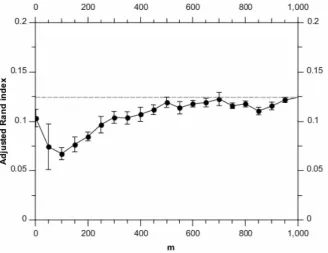
Figure 1 shows how the adjusted Rand index (averaged over runs) varies with the randomised algorithm parameter, m. For mv500, there is some loss in accuracy performance; however for
mw500, the adjusted Rand index is approximately that of the
greedy algorithm.
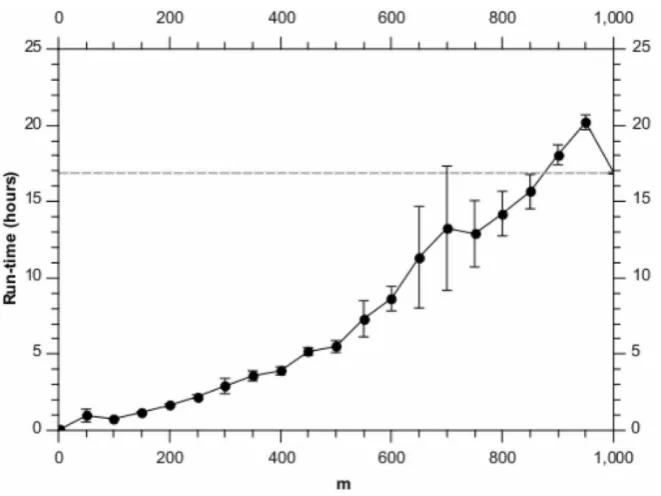
Figure 2 shows the corresponding run-time performance. As expected, the algorithm is approximately linear in m and a significant speed-up can be obtained over the greedy algorithm. For these synthetic data, one could therefore pickm~500and get approximately the same performance as for the greedy algorithm, but with more than a|2:5speed-up. And if some performance drop-off was acceptable, as much as an order of magnitude improvement is possible. We note that such a run takes only approximately 5 hours to complete on a single node 2.40 GHz Intel Xeon CPU.
We also consider how the run-time varies as a function of the total number of genes analysed,n. Figure 3 shows this variation for
several differentmvalues. Figure 4 shows the same information, expressed a a speed-up over the greedy algorithm.
We note an interesting effect for the lowest value ofm(m~10) in Figure 1. A significant part of the performance degradation for lowermvalues in Figure 1 comes from the randomised algorithm over-estimating the number of clusters (these being synthetic data, we know the ground truth number of clusters). Investigation of the m~10point shows that this effect is lessened for the synthetic data for smallm. We believe that this is because for small numbers of data items, the inferred noise level is more weakly constrained. This in turn allows for clusters with higher noise levels, meaning the algorithm can explain the data using a smaller number of noisy clusters.
Microarray Results
It is also important to validate the randomised algorithm on real microarray data. To do this, we use a subset of the data of [18], selecting genes that have a KEGG pathway annotation, using the version of the KEGG database to match that used in [20]. This consists of yeast cell cycle microarray time series for 1165 genes, measured at 17 time points.
As a performance metric, we choose the Biological Homoge-neity Index (BHI) [21], as implemented in the R package clValid [22]. The BHI metric scores a clustering partition between 0 and 1, with higher scores assigned to more biologically homogeneous partitions with respect to a reference annotation set. This has proven to be an effective metric for measuring the performance of microarray-based gene clustering [14,15].
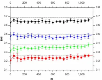
Figure 5 shows the BHI scores (averaged over 10 runs) as a function of the randomised-algorithm parameter, m. The BHI scores show very little variation for mw100, showing that the
[image:3.612.61.390.441.694.2]randomised algorithm is highly robust, in this case, to choice ofm. There is typically a small drop in performance relative to the greedy algorithm.
Figure 1. Adjusted Rand index scores for different values ofm, analysing the synthetic data set.Each point is the average of 10 runs, with the error bars denoting the standard error on the mean. The horizontal dashed line shows the result for the full BHC method.
doi:10.1371/journal.pone.0059795.g001
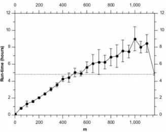
Figure 6 shows the corresponding run-times. As with the synthetic data, we see the expected O(m) scaling. We note that here the overhead of the randomised algorithm means that for mw600the greedy algorithm is actually faster. However, the BHI
[image:4.612.59.390.58.306.2]results in Figure 5 show that we could setm~200and gain almost a factor of 3 in speed while incurring only a minimal loss of performance. We note that such a run takes only approximately 2 hours to complete on a single node 2.40 GHz Intel Xeon CPU.
Figure 2. Run-times for different values ofm, analysing the synthetic data set.Each point is the average of 10 runs, with the error bars denoting the standard error on the mean. The horizontal dashed line shows the result for the full BHC method.
[image:4.612.57.391.427.694.2]doi:10.1371/journal.pone.0059795.g002
Figure 3. Run-time as a function of the number of genes,n, using (subsets of) the synthetic data.Shown are the results form~100(red),
Figure 4. Speed up factor as a function of the number of genes,n, relative to the full BHC method, using (subsets of) the synthetic data.Shown are the results form~100(red),m~200(green) andm~300(blue). The horizontal dashed line shows the full BHC result.
doi:10.1371/journal.pone.0059795.g004
Figure 5. BHI scores for difference values ofm, analysing the yeast microarray data set.Each point is the average of 10 runs, with the error bars denoting the standard error on the mean. The horizontal dashed line shows the results for the full BHC method. Shown are the results for the different gene ontologies, Biological Process (red), Molecular Function (green), Cellular Component (blue) and the logical-OR of all three (black). The BHI scores were all generated using the org.Sc.sgd.db annotation R package.
doi:10.1371/journal.pone.0059795.g005
[image:5.612.59.392.414.673.2]We note an interesting difference between Figures 2 and 6 in run time, relative to the greedy BHC algorithm. Because the number of genes is similar in both cases, one might expect the performance relative to the greedy algorithm to be similar. However (as is shown in these figures) the efficiency of the randomised BHC algorithm depends on how balanced (or otherwise) the dendrogram is. For example, if many levels of the dendrogram split into subsets of very different sizes (one big, one small), the randomised algorithm may have to go through many iterations in order to define the entire dendrogram. The run time is therefore dependent not only on the number of genes and time points, but also on the underlying clustering structure in the data. Essentially, unbalanced dendrograms make the randomised algorithm less efficient.
We also note that form values close to the actual number of genes, it is a general feature that randomised BHC will tend to be slower than the greedy algorithm. This is because in this case, the randomised algorithm has to perform a greedy run with almost the entire set of genes to define the top branching of the dendrogram, and then assign all the genes to one of the two branches and run the greedy algorithm again for each of these subsets.
Figures 2 and 6 show an increased variance in the run time for mw600. We believe this effect is due to the fact that for higher aˆJ,maˆJTM
values, the run time is more likely to be dominated by a single run of the greedy algorithm forDsubsetDvmitems. This
will make the run time very sensitive to DsubsetD, which will be affected by the randomisation of the overall algorithm.
Discussion
We have presented a randomised algorithm for the BHC clustering method. The randomised algorithm is statistically well-motivated and leads to a number of concrete conclusions.
N
The randomised BHC algorithm can be used to obtain a substantial speed-up over the greedy BHC algorithm.N
Substantial speed-up can be obtained at only small cost to the statistical performance of the method.N
The overall computational complexity of the randomised BHC algorithm isO(mnlogn).The randomised BHC time series algorithm can therefore be used on data sets of well over 1000 genes.
Use of the randomised BHC algorithm requires the user to set a value ofm. On the basis of the analyses presented in this paper, we recommend that a value ofmin the range100{200is reasonable, giving significant speed-up with minimal cost in terms of statistical performance.
The randomised time series BHC algorithm is available as part of the R package BHC, which is available for download from Bioconductor (version 2.10 and above) via http://bioconductor. org/packages/2.10/bioc/html/BHC.html.
We have also made available a set of R scripts which can be used to reproduce the analyses carried out in this paper. These are available from the following URL. https://sites.google.com/site/ randomisedbhc/.
Methods
[image:6.612.60.388.57.316.2]In this section, we provide a mathematical overview of the time series BHC algorithm. Greater detail can be found in [15]. time series BHC combines the BHC clustering algorithm, coupled with a Gaussian process data model to provide a flexible, generative representation of microarray time series. Here we replace the standard (greedy) BHC algorithm with a randomised algorithm, improving the computational complexity of the method and hence its run time for scientifically-useful numbers of genes.
Figure 6. Run-times for different values ofm, analysing the yeast microarray data set.Each point is the average of 10 runs, with the error bars denoting the standard error on the mean. The horizontal dashed line shows the results for the full BHC method.
BHC Algorithm
The BHC algorithm [13–15,23] performs agglomerative hierarchical clustering in a Bayesian setting. In agglomerative
[image:7.612.59.477.61.647.2]clustering algorithms, each gene begins in its own cluster and at each stage the two most similar clusters are merged. BHC uses a model-based criterion to do this, also learning the most likely
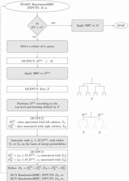
Figure 7. Flow chart showing the randomised BHC algorithm.The main loop is the randomised part of the algorithm, which is used recursively until the remaining gene subsets are small enough that it uses the greedy version of BHC to complete the tree and then terminates. doi:10.1371/journal.pone.0059795.g007
number of clusters given the data (something which many clustering methods are unable to do in a principled way). We note that the BHC algorithm can be interpreted as a fast approximate inference method for a Dirichlet Process Model (DPM) [13].
The prior probability,pk, that a given pair of clusters,C1and
C2, should be merged is defined by the DPM and is determined
solely by the concentration hyperparameter for the DPM and the number of genes currently in each partition of the clustering. Bayes’ rule is then used to find the posterior probability,rk, that the pair of clusters should be merged,
rk~
pkP(yDH1k)
P(yDTk)
, ð1Þ
where y~fy1,. . .,yNg is the set of N data points contained in clustersC1andC2.P(yDH1k)is the marginal likelihood of the data
given the hypothesis,Hk
1, that the dataybelong to a single cluster
and requires the specification of a likelihood function, f, as the probabilistic model generating the observed data,y.P(yDTk)is the probability that the data could be partitioned in any way which is consistent with the order of assembly of the current partition and is defined recursively,
P(yDTk)~pkP(yDHk1)z(1{pk)P(yDTi)P(yDTj), ð2Þ
whereTiandTjare previously merged clusters containing subsets of the data iny.
Whenrkis greater than 0.5, it is more likely that the data points contained in the clustersC1andC2were generated from the same
underlying function,f, than that the data points should belong to two or more clusters. Whenrk is less than 0.5 for all remaining pairs of clusters, the number of clusters and partitions best described by the data has been found.
For the purposes of the BHC algorithm, a complete dendro-gram is constructed, with at each step the most likely merger being made. This allows us to see the log-probability of mergers in the whole dendrogram, even when this value is very small. To determine the likely number of clusters, given the data, we then cut the dendrogram wherever the probability of merger falls below 0.5 (i.e. non-merger is more likely).
As described in [13], thepkare dependent on a hyperparameter for the mixture model,a. As in previous work on BHC, we set
a~0:001as a fixed value. This has the effect of setting a prior assumption of only weak clustering. One could learn this parameter as part of the BHC algorithm; we choose to not do this as it will substantially increase the run time of the algorithm. The BHC algorithm provides a lower bound of the DP marginal likelihood, as shown in [13]. For the randomised algorithm, we note that the lower bound on the DP marginal likelihood is effectively determined using a subset of onlymdata items. These lower bounds are used in the usual way to optimise hyperpara-meters for each potential merger. One could attempt in principle to compute the lower bound using allndata items. However, this will be computationally intensive and so we do not consider it in this paper.
Gaussian Process Regression
Gaussian processes define priors over the space of functions, making them highly suited for use as non-linear regression models. This is highly valuable for microarray time series [24–27], where a wide range of functional forms can be expected. In essence, Gaussian Process Regression (GPR) allows us to minimise the
assumptions we must make as to the underlying structure in our time series data.
For the time series BHC model, we model an observation at timetiasy(ti)~f(ti)ze. For each cluster, we assume the latent function f is drawn from a Gaussian process with covariance functionS, defined by hyperparameters,hS. We also assumeiid
Gaussian noise,N(0,s2 e).
Lety~½y1,1. . .yG,tbe theN~G|Tobservations in a cluster of Ggenes, where the fyg,tgare time series of f1,. . .,Tgtime points. Each gene is normalised to have mean 0 and standard deviation 1 across time points. The prior off is given for fixed values of hS, such that P(fDhS)~N(0,S). It follows that the
likelihood function forf isP(yDf,s2
e)~N(f,s2eI), whereI is the
N|N identity matrix. The marginal likelihood of the data, y, is then:
P(yDhS,s2e)~N(0,Szs2eI) ð3Þ
~(2p){N2DKD{12exp({1 2y
T(K){1y) ð4Þ
whereK~Szs2
eIis the covariance function fory.
Time series BHC implements either the squared exponential or cubic spline covariance functions. In this paper, we restrict our attention to the default choice of squared exponential covariance:
KSE(ti,tj)~s2f exp({
(ti{tj)2
2l2 )
" #
zs2
edij ð5Þ
wheredijis the Kronecker delta function andtiandtjare two time points forf.s2
f is the signal variance parameter for the covariance function andlis the length-scale parameter.
Randomised BHC Algorithm
To speed up the time series BHC, we implement the randomised BHC algorithm of [17] (specifically, algorithm 1). The key insight from which we hope to benefit is that the standard, greedy BHC algorithm is dominated by the computation of merges at the lowest level of the tree. Therefore, if we can reduce this load in a sensible way, it may be possible to produce a substantially faster algorithm.
Throughout this paper we will refer to the top of the
dendrogram. This is the highest level of the dendrogram, where the whole set of genes is split into two subsets.
For reasonably balanced trees, the top levels should be well-defined even using only a random subset of the genes. From this idea, we can define the following randomised algorithm.
N
Select a subset ofm%ngenes.N
Run BHC on the subset ofmgenes.N
Filter the remaining(n{m)genes through the top level of the tree, computing merge probabilities between each individual gene and the two subsets ofmto decide to which branch the gene belongs.N
Including the original m genes, we have now subdivided all genes on the basis of the top level branch of the tree.In effect, we are using estimates of the higher levels of the tree to subdivide the genes so that it is not necessary to compute many of the potential low-level merge probabilities. Figure 7 shows a flow chart describing the algorithm.
Setting the Hyperparameters
The covariance function of the Gaussian processes used in this paper are characterised by a small number of hyperparameters. These hyperparameters are learned for each potential merger using the BFGS quasi-Newton method [28].
This merge-by-merge optimisation allows each cluster to have different hyperparameter values, allowing for example for clusters with different intrinsic noise levels and time series with different characteristic length scales.
Utilising the Covariance Matrix Block Structure
We assume in this paper that each time series is sampled at the same set of time points. This leads to a block structure in the covariance matrix, which can be utilised to greatly accelerate the computation of the Gaussian process marginal likelihood.
The computational complexity of BHC is dominated by inversion of the covariance matrix. Considering the case of a group ofk genes, each sampled at the same T time points, the naive approach to matrix inversion would require us to invert a kT|kT matrix, which is an O(k3T3) operation. However, we
can instead use block matrix pseudoinversion, which recursively reduces the block size to one, at which point the remaining inversion is anO(T3)operation.
We also note that this is equivalent to a Bayesian analysis using a standard multivariate Gaussian. Indeed, considering the task in this way may be a simpler way of doing so and is certainly a useful way of gaining additional insights into the workings of the model.
Computational Complexity
When proposed merges have constant cost (the case considered by [17]), the standard greedy BHC algorithm has O(n2)
computational complexity.
For the time series BHC algorithm however, the merges do not have have constant cost. For a given node, we are mergingkgene time series, each of lengthT. We therefore have to consider a
(kT)|(kT)covariance matrix, which we must invert. As noted in [15], this matrix is actually a block matrix consisting of k|k blocks, which means we can invert it inO(kT3)operations.
Becausekwill be as large asnfor the merges closer to the root node of the tree, this gives the greedy time series BHC algorithm a worst-case computational complexity ofO(n3T3).
The randomised algorithm for case of constant cost merges has O(nlogn) complexity [17]). Heller and Ghahramani show that, for reasonably balanced trees, the complexity is dominated by the filtering step. Each of theO( logn)filtering steps isO(n), resulting in the overall O(nlogn) complexity. For the time series BHC algorithm, the filtering step isO(nmT3), because of the additional
cost of merging time series clusters. As in the original analysis there will beO( logn) filtering steps, giving an overall computational complexity for the randomised version of time series BHC of O(mT3nlogn).
Acknowledgments
We thank Jim Griffin for useful discussions.
Author Contributions
Conceived and designed the experiments: RD RSS EJC ZG PDWK DLW. Performed the experiments: RD. Analyzed the data: RD RSS EJC PDWK DLW. Contributed reagents/materials/analysis tools: RD RSS. Wrote the paper: RD RSS EJC ZG PDWK DLW.
References
1. Bauwens L, Rombouts J (2007) Bayesian clustering of many garch models. Econometric Reviews 26: 365–386.
2. Fru¨hwirth-Schnatter S, Kaufmann S (2008) Model-based clustering of multiple time series. Journal of Business and Economic Statistics 26: 78–89. 3. Jackson E, Davy M, Doucet A, Fitzgerald W (2007) Bayesian unsupervised signal
classification by Dirichlet process mixtures of Gaussian processes. In: Acoustics, Speech and Signal Processing, 2007. ICASSP 2007. IEEE International Conference on. IEEE, volume 3, pp. III–1077.
4. Eisen M, Spellman P, Brown P, Botstein D (1998) Cluster Analysis and Display of Genome-wide Expression. Proceedings of the National Academy of Sciences 95: 14863–14868.
5. Schliep A, Costa IG, Steinhoff C, Schonhuth A (2005) Analyzing gene expression time-courses. IEEE/ACM Trans Comput Biol Bioinform 2: 179– 193.
6. Beal M, Krishnamurthy P (2006) Gene Expression Time Course Clustering with Countably Infinite Hidden Markov Models. In: Proceedings of the Proceedings of the Twenty-Second Conference Annual Conference on Uncertainty in Artificial Intelligence (UAI-06). Arlington, Virginia: AUAI Press, 23–30. 7. Bar-Joseph Z, Gerber G, Gifford D, Jaakkola T, Simon I (2003) Continuous
representations of time-series gene expression data. Journal of Computational Biology 10: 341–356.
8. Heard NA, Holmes CC, Stephens DA, Hand DJ, Dimopoulos G (2005) Bayesian coclustering of Anopheles gene expression time series: Study of immune defense response to multiple experimental challenges. Proceedings of the National Academy of Sciences 102: 16939–16944.
9. Heard NA, Holmes CC, Stephens DA (2006) A Quantitative Study of Gene Regulation Involved in the Immune Response of Anopheline Mosquitoes: An Application of Bayesian Hierarchical Clustering of Curves. Journal of the American Statistical Association 101: 18.
10. Ma P, Castillo-Davis CI, Zhong W, Liu JS (2006) A data-driven clustering method for time course gene expression data. Nucleic Acids Research 34: 1261– 1269.
11. Liverani S, Cussens J, Smith JQ (2010) Searching a Multivariate Partition Space Using MAXSAT. In: Masulli F, Peterson L, Tagliaferri R, editors, Computa-tional Intelligence Methods for Bioinformatics and Biostatistics, 6th Interna-tional Meeting, CIBB 2009 Genova, Italy, Springer, Heidelberg, volume 6160 of Lecture Notes in Computer Science. 240–253.
12. Bar-Joseph Z (2004) Analyzing time series gene expression data. Bioinformatics 20: 2493.
13. Heller KA, Ghahramani Z (2005) Bayesian Hierarchical Clustering. In: Twenty-second International Conference on Machine Learning (ICML-2005). 14. Savage RS, Heller K, Xu Y, Ghahramani Z, Truman WM, et al. (2009) R/
BHC: Fast Bayesian Hierarchical Clustering for Microarray Data. BMC Bioinformatics 10: 242.
15. Cooke E, Savage R, Kirk P, Darkins R, Wild D (2011) Bayesian hierarchical clustering for microarray time series data with replicates and outlier measurements. BMC Bioinformatics 12: 399.
16. Motwani R, Raghavan P (1995) Randomised Algorithms. Cambridge University Press.
17. Heller K, Ghahramani Z (2005) Randomized algorithms for fast bayesian hierarchical clustering. PASCAL Workshop on Statistics and Optimization of Clustering 25: 1–22.
18. Cho R, Campbell M, Steinmetz EWL, Conway A, Wodicka L, et al. (1998) A Genome-Wide Transcriptional Analysis of the Mitotic Cell Cycle. Molecular Cell 2: 65–73.
19. Hubert L, Arabie P (1985) Comparing partitions. Journal of the Classification 2: 193–218.
20. Savage RS, Ghahramani Z, Griffin JE, de la Cruz BJ, Wild DL (2010) Discovering Transcriptional Modules by Bayesian Data Integration. Bioinfor-matics 26: i158–i167.
21. Datta S, Datta S (2006) Methods for evaluating clustering algorithms for gene expression data using a reference set of functional classes. BMC Bioinformatics 7: 397.
22. Brock G, Pihur V, Datta S, Datta S (2008) clValid: An R package for cluster validation. Journal of Statistical Software 25: 1–22.
23. Xu Y, Heller K, Ghahramani Z (2009) Tree-based inference for Dirichlet process mixtures. AISTATS 2009 conference.
24. Chu W, Ghahramani Z, Falciani F, Wild DL (2005) Biomarker discovery in microarray gene expression data with Gaussian processes. Bioinformatics 21: 3383–3393.
25. Kirk PDW, Stumpf MPH (2009) Gaussian process regression bootstrapping: exploring the e_ect of uncertainty in time course data. Bioinformatics 25: 1300– 1306.