Optimization of a control network for binding in combinatorial sentence structures

(1)

MASTER THESIS

Optimization of a control network

for binding in combinatorial

sentence structures.

Koen Meijer, s1744275

Faculty of Cognitive Psychology and Ergonomics Human Factors and Engineering Psychology

EXAMINATION COMMITTEE

Prof. F. van der Velde & Dr. M. Schmettow.

(2)

2

Optimization of a control network for binding in combinatorial

sentence structures.

Koen Meijer, s1744275

Date: 1-8-2019

Supervisors: Prof. F. van der Velde & Dr. M. Schmettow.

Human Factors and Engineering Psychology

(3)

3

Abstract

The ability of human to understand and produce combinatorial structures in language is an

important feat of cognition. It allows for the understanding of a huge set of sentences

generated by the combination of a known sentence structure and known words. How these

combinatorial structures can be instantiated in neural terms is still faced by some challenges. The neural blackboard architecture (NBA) aims to solve these challenges. In this architecture

words are bound together in a temporary sentence structure that encodes the relations between

the words. The question remains with what network the binding in the NBA can best be

controlled. Therefore, the goal of this thesis was twofold. The first being the replication of the

FFN trained by van der Velde and de Kamps (2010). The second being finding the best

hidden layer size for this FFN. Accuracy as reported by Keras showed a decline for

processing of the test sentences for the models with six or fewer hidden nodes. However, a

model configuration that completely omitted the hidden layer scored an accuracy equal to the

model with 12 hidden nodes. Further inspection of the activations made by the models

revealed that the model without a hidden layer made more errors. In conclusion it can be said

that a model without a hidden layer is not adequate to perform the controlling task for binding

in the NBA if the performance requirements of van der Velde and de Kamps (2010) are

applied. However, when the standard Keras thresholds for accuracy are used the model

without a hidden layer seems to be able to control the binding. This points towards the data

(4)

4

1. Introduction

Language comprehension or semantic cognition is the ability to use, manipulate and

generalize knowledge to support both verbal and non-verbal behaviours (Lambon-Ralph,

Jefferies, Patterson & Rogers, 2017). A fundamental characteristic of human semantic

cognition is that it relies on combinatorial structures. Humans use combinatorial structures in language by combining vowels and consonants into syllables, syllables into words and words

into sentences (Zuidema & de Boer, 2018). This ability is almost unending as humans can

always create new words using known phonemes and can express complex thoughts using

new combinations of words forming novel sentences. This combinatorial productivity even

results from combining simple sentence structures with a large but finite lexicon. It is not

unlimited but still results in a huge set of sentences that can be understood because this results

from combining a finite lexicon with restricted sentence structure. When new words are

learned in a particular sentence context, these words can also be recognized in other sentence

contexts without explicitly learning these first. Adult language users possess this form of

productivity. Thus, with combinatorial productivity new words only have to be learned in a

few sentence contexts. They could then be used in other sentence context as well..

Studying how these combinatorial structures can be instantiated in neural terms is

essential to understanding the basis of human cognition. The representation of words and

concepts are formed by neural cell assemblies (Hebb, 1949). Such an assembly consists of a

group of interconnected neurons that is distributed across the brain. The hub and spokes

model of semantic cognition (Lambon-Ralph et al., 2017) is a more recent version of this

hypothesis. In this model semantic cognition relies on two interacting neural systems. The

first system is a system of representation in which knowledge of concepts is encoded. The

second system manipulates the activation within the first system and is therefore a system of

control. This two systems view is called the controlled semantic cognition (CSC) framework

(Lambon-Ralph et al., 2017). However, the neural instantiation of the combination of such

structures poses some fundamental problems. These problems are the massiveness of binding,

the problem of two, the problem of variables and the transformation of combinatorial

structures from working memory to long-term memory (Jackendoff, 2002). The Neural

Blackboard Architecture (NBA) (van der Velde & de Kamps, 2006) can solve these

challenges to cognitive neuroscience. Moreover, this is a neural architecture that aims to

integrates three important features of human cognition. These features are productivity,

(6)

6 described above. Dynamics refers to the ability of interacting with the environment in a

dynamical way. Grounding refers to the nature of cognitive representations.

These representations are always grounded in perception. Especially the combination of these

features is important to human cognition and not found often, except in the human brain.

Therefore, to better understand the nature of human cognition an architecture that integrates

these features is important (van der Velde & de Kamps, 2006). The NBA can create

combinatorial structures. However, without a control network that has learned in which way

to activate certain structure assemblies the NBA is not capable of processing novel structures.

A control network is therefore needed to make the model capable of productivity.

Once a specific sentence structure is learned; let’s say a N-V-N structure, this can be

generalized to all sentences of this type as long as it consists of nouns and verbs that are

known to the human/model. So the need to train a neural network on a significant number of

sentences of the overall set humans can understand can be avoided (van der Velde, van der

Voort van der Kleij & de Kamps, 2004). In this study a control network for a model of

sentence structure will be tested. This control network will provide the necessary input for the

NBA (van der Velde & de Kamps, 2006) to make it capable of processing novel sentences.

Further testing with the control network will determine whether it is capable of processing the

combinatorial structures in the same way as humans. A control network could make the NBA

capable of processing novel sentences just like humans are able to process and produce

combinatorial structures (van der Velde & de Kamps, 2006). The first part of this of thesis

will be dedicated to replicating the study by van der Velde and de Kamps (2010) on learning

of control in a neural architecture of grounded language processing. The second part will

consider trying different configurations of the model to optimize the performance. Mainly, the

(7)

7

2. Theoretical framework

2.1 Combinatorial productivity/structures.

The combinatorial nature of language refers to the way human combine sounds to

form word (combinatorial phonology) and the way in which humans combine words into

sentences (compositional structures) (Zuidema & de Boer, 2018). In this way humans can

combine words to form novel sentences, as long as the words are known.

The ability to provide ‘who does what to whom’ information can be seen as the

communicative aspect of language. Two sentences with the same syntactic structure can give

very different information. By answering who does what to whom question this information

can be derived. This is called a binding question since it is related to the manner in which the

constituents in the sentence structure are bound together. For instance, the information in a

sentence changes meaning when a noun goes from the object to the subject position.

Answering such binding questions is an important feature of human language processing (van

der Velde, van der Voort van der Kleij & de Kamps, 2004).

Human language processing is very productive in representing who does what to

whom information. With a vocabulary of 1000 words and one specific sentence structure a

huge set of sentences can be created. Every human that knows the words that are in the

vocabulary and is familiar with the specific sentence structure can then understand each

sentence in this set and would be able to answer binding questions. The combinatorial

productivity of language results from combining sentence structures with a large lexicon (vocabulary). This will result in a set of sentence which is ‘astronomical’ in its size but still

understandable to the average person because they are the result of combing a large but finite

lexicon with restricted sentence structures (van der Velde, van der Voort van der Kleij & de

Kamps, 2004). To deal with learning a set of this size combinatorial productivity in a model is

also needed. This way, not every combination of words and sentence structures has to be

trained but new words can be trained in a few contexts and then used in others. Or a model

can learn different sentence structures without simultaneously learning specific words.

The ability of a model to learn a specific word in one type of sentence and then use it

in another is a form of productivity referred to as strong systematicity. However, this type of

systematicity could be difficult for a neural network to learn because the word as well as the

syntactic position have to be learned at the same time. Moreover, for combinatorial

productivity strong systematicity may be not be necessary. Alternatively, a form of weak

(8)

8 sentences may be sufficient to produce combinatorial productivity (van der Velde, van der

Voort van der Kleij & de Kamps, 2004).

2.2 Grounded representations

A grounded representation of a specific word is made up from all the related aspects to

that word in an interconnected network. The aspects that are related include perceptual

information, processes related to actions (petting a cat), emotional information related to the

word and all other forms of information.

Several studies have investigated grounded word representations in the brain. One

interesting finding is that of modality specific activation in the brain during the

comprehension of words. Motor related words activated brain areas that are associated with

motor skills and sensory brain areas where activated during the comprehension of sensory

related words (Vigliocco et al., 2006). Difference in activation between several words related

to motor action were also found. Parts of the premotor cortex that are activated by specific

actions were activated by words related to these specific actions (Tettamanti et al., 2005).

The hub-and-spoke theory of semantic representations explains how conceptual

knowledge can arise. This theory assumes that the most important sources for constructing

concepts are multimodal verbal and non- verbal experiences. These sources of information are

encoded in modality specific brain areas that are distributed across the brain. These are called

the spokes. The second idea of this theory is that interactions across modalities are mediated by a trans-modal hub that is situated bilaterally in the anterior temporal lobes (ATL)

(Lambon-Ralph et al., 2017).

There is empirical evidence that motivates that the hub is situated on the anterior

temporal lobes, mainly from cognitive neuropsychological studies. Damage to higher-order

association cortices can lead to trans-modal semantic impairments. An interesting study on

semantic dementia (SD) showed that the ATL-hub might be important for all types of

concepts. Patients with SD show atrophy and hypometabolism in the anterior temporal

regions bilaterally. With semantic SD there are impairments across all modalities and all types

of concepts. This seems to point towards a central, trans-modal hub (Lambon-Ralph et al.,

2017).

2.3 Recurrent Neural Networks and combinatorial productivity

Recurrent neural networks can be used to study sentence processing. An example of

(9)

9 (Elman, 1991). A SRN is essentially a multilayer neural network with connections between

the input layer and hidden layer and the hidden layer and output layer. Recurrence is made

possible by copying information from the hidden layer back to the input layer. This is done

via the context nodes as shown in figure 1. The information that is stored in the context layer

is combined with the next input. In this way the hidden layer of the model relates both new

and prior information to the output layer (Elman, 1991). This model was trained on a set of

sentences so that it could predict the lexical category of the next word in a new sentence.

In a more recent study a SRN was used to examine whether such a model would be

capable of combinatorial productivity (van der Velde, van der Voort van der Kleij & de

Kamps, 2004). However, the model that was used failed on the test of combinatorial

productivity. The SRN was capable of learning the training sentences but with the test

sentences in which words from the learned sentences were combined it failed to correctly

predict the lexical category of the next word. In their article they call this a falsification of the

idea that a SRN can manage human language productivity (van der Velde & de Kamps,

2004).

Figure 1: A simple recurrent neural network (van der Velde, van der Voort van der Kleij & de Kamps, 2004).

Combinatorial productivity is not the same as recursive productivity. Recursive

productivity refers to processing increasingly complex structures whereas combinatorial

productivity concerns combining a big lexicon with limited syntactic structures (van der

Velde & de Kamps, 2006). The long short-term memory recurrent network has, as opposed to

SRN and humans, unlimited recursive productivity. It can also handle context free language by using ‘memory units’ that work as counters during learning. However, counting elements

(10)

10 is encountered in a sentence differences between sentences cannot be represented.

Additionally, this method would not work for new sentences with words that have not been

encountered before and therefore do not have a counter yet. This shows that the ability to

process increasingly complex languages does not assure that combinatorial productivity can

also be processed (van der Velde & de Kamps, 2006).

Another issue with a SRN is related to the binding problem, which entails the way in

which the structural relations between parts can be kept when these parts are bound together

momentarily. Instead of processing words directly a SRN could be trained to process

sentences based on their abstract structure. The problem with this however would be that all

sentences with the same syntactic structure, such as Noun-Verb-Noun would be the same for

this model even though they convey different messages. Humans have the ability to answer

binding questions for this type of sentence but these questions are impossible to answer based

solely on the abstract sentence structure. To be able to distinguish the different messages of

sentence with a similar abstract structure the binding has to be performed according to the

hierarchical structure of the sentence. This is a form of language processing of which a SRN

is not capable (van der Velde & de Kamps, 2006).

2.4 The Neural Blackboard architecture of combinatorial structures.

In a combinatorial structure parts and their relations are both present. This means that

a neural model of combinatorial structures can only be useful when it instantiates the

individual parts as well as the relations between them in a combinatorial structure. Moreover,

in a sentence structure the individual parts consist of the grounded word representations as

described in the hub-and spoke model (Lambon-Ralph et al., 2017). The combination of

combinatorial productivity with grounded word representations presents challenges. It means

that connections should be possible between all of the different grounded representations of

nouns and all grounded representations of verbs. Additionally, connections between these

grounded representations cannot be formed directly when a new combination of nouns and

verbs is encountered. Therefore, combinatorial productivity has to be possible in a connection

structure that is already established (van der Velde, 2019).

The neural blackboard architecture makes this combination possible by forming a

temporary connection between arbitrary nouns and verbs (van der Velde & de Kamps, 2006).

This temporary connection structure is formed on a ‘blackboard’ consisting of specialized

processors that can interact. Each of these processors can process and alter the information on

(11)

11 the grounded word representations in a sentence structure. There are noun assemblies and verb assemblies. When a sentences is processed all the nouns are linked to an individual noun assembly and the verbs are linked to verb assemblies. The noun and verb assemblies are

linked together in a manner that encodes the relations between these words. Within the

structure assemblies for nouns and verbs are subassemblies for the different roles these words

can have in a sentence structure. For example, for the sentence dog sees cat, dog and cat are linked to two different noun assemblies. Sees is linked to a verb assembly. Next, these

assemblies are linked together by the appropriate subassemblies. Dog is linked as the agent of sees, and cat as the theme of sees. This linking of structure assemblies in the NBA is called binding. The binding in the architecture is achieved by activating the correct binding gates in

the structure assemblies (for a detailed description of binding gates in the NBA sees van der

Velde & de Kamps, 2006).

In the NBA the activation of binding gates needs to be controlled. A control network

for this task was proposed by van der Velde and de Kamps (2010). This network received

information about the word types in a sentence structure and feedback from the NBA

concerning expectations of the sentence structure. For instance, verbs usually have themes

therefore when a theme is encountered this is signalled to the control network. How this

control works is discussed in detail in the next section.

2.5 Control of binding in the Neural Blackboard Architecture

In a recent study a control network for the neural blackboard architecture was

presented (van der Velde & de Kamps, 2010). The network that was used to control the

binding was a feedforward network (FFN) with one hidden layer that operated on abstract

binding symbols. These binding symbols/categories could then be used to activate the

appropriate structure assemblies in the NBA. The main goal of this study was to investigate

whether a neural network is capable of generalizing knowledge of these binding classes to

novel sentence structures. To this intent two main types of sentences were trained. Namely,

sentences with a noun-verb-noun structure and sentences with an embedded clause. Below is

a description of the input-output relations the FFN learned to control the binding.

During binding, nodes are activated that represent a lexical category. This is done

from the assumption that grounded word representations also entail information about lexical

categories. For the noun-verb-noun sentences there are several of these categories that were

uses to train the control network on the binding steps. These are nouns with a relative clause

(12)

12 there are two categories that are meant for starting and ending sentence structures in the NBA

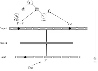
and there are conditional nodes. Figure 4 shows the binding steps for the sentence cat sees dog. For each word in this sentence ate least one or more nodes in the input- and output layer are activated. All the necessary steps in the binding process for this sentences is discussed

below.

The FFN that was trained operates on sentence level in which the parts of the sentence

structure are processed word for word. The first action is that cat activates an input node in the FFN. This does not happen directly but rather by recognizing the category to which cat belongs first. In the case of cat this category is noun with a possible relative clause (Nrc). In the input layer of the FFN there is a node dedicated for signalling the to the output layer that

the input is Nrc. The trained model has learned to activate the correct output in this case. The

correct output that needs to be produced by the FFN consists of two nodes. The first is for

activating the noun cat as the subject of the sentence (N-n-S). This node will signal to the NBA that these two structure assemblies are bound together via their noun-subassemblies. Cat (N1) will then be bound to the sentence structure (S1) as the subject. Additionally, the FFN

has learned to activate a node that reflects the expectation of an incoming relative clause

(RC). This is an example of a conditional node that is not used as input for the model directly.

Rather, it is used as feedback for the FFN. The RC node will serve as input together with a

(13)

13

Figure 2: Schematic presentation of the processing of a noun with possible relative clause Cat through the FFN. Dots represent nodes in the input- and output layer; black dots are nodes that are activated.

The verb sees falls under the verb category which activates the V node in the input layer of the FFN as displayed in figure 3. The trained FFN has learned to activate two nodes

for verb inputs. The first is the V-v-S node. When this node is activated it signals to the NBA

that the verb (V1) should be bound to the sentence structure (S1) as a verb. Since verbs

usually have a theme an additional node is activated in the output layer of the FFN. The V-t

node reflects the expectation that the next word in the sentence structure could be the theme

of the verb sees. In the NBA, the result is that a gate is opened for theme-subassembly in the V1 structure assembly. A feedback signal is also produced. The conditional node T is

activated and will remain active until new input will satisfy the condition of being a theme

[image:13.595.80.466.364.643.2]

(van der Velde & de Kamps, 2010).

Figure 3: Binding of the verb sees as the verb of the sentence structure cat sees dog. The anticipation of a theme is reflected by the V-t node and the conditional T node which is given

(14)

14 The last word of the sentence, dog, is another noun with a possible relative clause (Nrc). Therefore, similarly to the first noun cat the Nrc node in the input layer of the FFN is activated. However, this time another node in the input layer is active. The conditional T node

that was given as feedback after processing the verb sees is also active. The FFN has learned to activate two nodes in this case. The RC node for a possible incoming relative clause and

the N-t node. This N-t node signals that the noun dog is a theme and therefore the theme subassembly of N2 should be activated. Together with the theme subassembly of V1 this

forms the binding of dog as the theme of the verb sees. Since the condition of the T conditional node is now met it is no longer activated and therefore not given as feedback

[image:14.595.77.430.303.579.2]

again (van der Velde & de Kamps, 2010).

Figure 4: Activation in the FFN for the noun dog in the sentence cat sees dog. The result is that dog is bound as the theme of the verb sees. Black circles represent activated nodes in the in-and output layer.

2.6 Research aims

The first aim of this study was to replicate the results by van der Velde and de Kamps

(15)

15 sentences and sentences with an embedded clause. After training the model was evaluated to

see if it is capable of controlling the binding task similarly to the original model.

After the replication of model the second aim was to evaluate the effect of hidden the

layer size on the performance of the model. In the original study the number of hidden nodes

was chosen without explicit thought. Therefore, the hidden layer size was lowered from the

original size of 12 nodes until a model was created without a hidden later at all, called a

perceptron. All of these architectures will be discussed in the sections below.

In the original study the number of epochs for training was set to 50.000. However,

this number was chosen without a specific reason. Therefore, during the evaluation the

number of epochs and the extent to which training for 50.000 epochs is necessary for the

binding task was also evaluated.

The last research aim is related to the tools that were used in the original study. At that

time software packages such as Keras were not available for use. Keras provides a clear

framework for creating neural networks and makes it more accessible to be used by those who

(16)

16

3. Network architectures

A Feedforward Neural Network for classification was used to serve as a control

structure for the Blackboard architecture. The code for this model can be found in appendix 1.

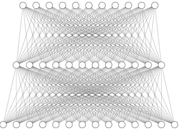
This type of network is also called a Multilayer Perceptron and is illustrated with figure five.

It consists of three densely connected layers of which the middle is the ‘hidden layer’. The

first layer is the input layer and contains eleven nodes or neurons. Each neuron in the input layer is connected to each neuron in the hidden layer. In turn each neuron in the hidden layer

is connected to the neurons in the output layer that consist of 14 nodes. In this way the neurons can take the input data or the output of other neurons as input. These data are then

multiplied by the neurons weight. This is initially a random number but through optimization the weight is adjusted so that the prediction of the model becomes closer to the desired value.

This is done by calculating a distance value to the true score, the loss value. The gradient of the loss is calculated and the parameters of the network are moved in the opposite direction of

the gradient (Chollet, 2018). This way the combination of weights in the network that creates

the smallest loss value can be found. These computations involve a series of computations to

[image:16.595.76.440.425.697.2]

calculate the gradient, called backpropagation. The process of optimizing the network based on these computations is called stochastic gradient descent (Chollet, 2018).

(17)

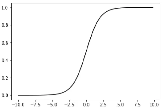
17 As the activation function in the last layer of the network the Sigmoid function was

used. The sigmoid function is defined as:

𝑓(𝑥) =

1 1 − ⅇ

−𝑥

The sigmoid function has a distinctive s-shape as shown in figure six. This shows that the sigmoid function is a ‘squashing function’. A large range of values are squashed into the

range of 0 and 1. This value indicates the probability that a given input belongs to a certain

output class. Since this value is calculated for each neuron in the output layer separately this

function can handle the data used to train the model. The classification task that needs to be

performed to control the binding in the blackboard architecture is one in which each input can

be related to multiple output categories simultaneously. This is called a multi-label

[image:17.595.74.339.320.501.2]

classification task.

Figure 6: The sigmoid function

All of the FFN models that were used in this study only differ with respect to the size

of the hidden layer. The middle section of the connections structure in figure five becomes

smaller as the number of nodes decreases. This also decreases the number of connections that

are made between the three layers. The final model that was tested consisted of only two

layers, an input and an output layer. This connection structure is pictured in figure 11. Such a

connection structure in which the input directly passes through to the output layer is called a

perceptron model. The process through which a perceptron model learns is different compared

to that of the FFN model described above. A perceptron model does not have a hidden layer

of neurons. It can only handle data that can be separated in a linear manner. This is directly related to the classification task a model needs to perform. There are two forms of

(18)

18 AND and OR classification. These two types of classification will be illustrated with a

perceptron model consisting of two layers illustrated in figure seven. In the first layer there

are two neurons; x and y. The last layer consists of 1 neuron which is the output of the model.

[image:18.595.72.222.521.655.2]

All of the neuron can have a value of 1 or 0.

Figure 7: Simple perceptron with two input nodes: x and y.

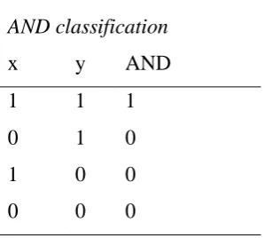
For the AND classification the neuron in the output layer will have a value of 1 if both

the x and y neuron have a value of 1. This gives the following input space as shown in figure

8. In table 1 the result of the different combination of x and y on with the AND classification

are given. These points can be plotted as x,y coordinates. In figure eight this is translated to a

dot for the output value being 0 and triangle for an output value of 1. The red line shows that

for this input space, a linear line can separate the dots from the triangle.

Table 1.

AND classification

x y AND

1 1 1

0 1 0

1 0 0

0 0 0

Figure 8: Input space for AND classification. A single line can separate the two classes: dots and

(19)

19 The second example of classification that a perceptron model can handle is OR

classification. In this case the output of the model becomes 1 when either the x or y node is a

1. This gives the following output as sees in table 2. In contrast to the AND classification this

type of classification results in more values of 1. In figure nine this translates to more

triangles. However, the triangles can still be separated from the dots with one linear line.

Figure 9: Input space for OR classification. This type of classification is linearly separable as shown by the red

line separating the triangles from the dot.

The exclusive/or (EXOR) classification however cannot be separated in a linear

manner and can therefore not be classified by a perceptron model. For this classification task

the output neuron in the perceptron neuron should take the value of 1 if only x or only y has a

value of 1. Figure 10 shows that a single line cannot separate the two classes in the input

space.

Figure 10: Input space for EXOR classification. Not linearly separable with a single line.

Table 2.

OR classification

x y OR

1 1 1

0 1 1

1 0 1

0 0 0

Table 3.

EXOR classification

x y EXOR

1 1 0

0 1 1

1 0 1

(20)

20 The data used in this study was assumed to not be linear separable and therefore it was

expected that this perceptron model could not correctly serve as a control network for the

NBA. The perceptron model that was used is shown in figure 11. An input layer with 11

nodes, one for each class in the input data is directly connected to the output layer of 14

nodes. Again, there is one node for each class of the output data. The specific classes in the

dataset are discussed in the next section.

(21)

21

4. Method

In this section the specific in- and output data that were used to model the binding

tasks are described. The training and test sentences are given and the way they were encoded

to be used by the model is explained. Lastly, the procedure of training the networks and the

way in which the networks were evaluated is reported.

4.1 Categories in the in- and output data

The number of nodes in the in-and output layers of the FFN and perceptron model

correspond to the number of binding categories that were used. For the input data the different

categories and the corresponding nodes in the model are given in table four. The first two

nodes in the input layer are dedicated to starting and ending sentences structures. Similar to

the study by van der Velde & de Kamps (2006) there are nodes for nouns with a possible

relative clause, nouns with a complement clause, verbs and clauses. In addition to these nodes there are five conditional nodes. These conditional nodes cannot be input to the network

directly but have to be activated by output first. They then remain active until input either

satisfies the condition for the conditional node or new input terminates the activation of the

conditional node. An example of how this works is described above in the section on control

in the NBA.

Table 4.

Binding categories in the training data

Input layer FFNN

Symbol Meaning Node number

B Begin S 1

E End S 2

Nrc Noun with possible relative clause 3

Ncc Noun with possible complement clause 4

V Verb (all verbs have themes) 5

C Clause (clause word: that, who) 6

T Theme conditional node 7

CC Complement Clause conditional node 8

CV Clause-verb conditional node 9

CT Clause-theme conditional node 10

(22)

22 For the output layer the first two nodes are dedicated for activating and deactivating

structure assemblies. In table five the categories and their corresponding node number are

presented. Next there two nodes that encode a noun as either the subject of the sentence as a

whole (N-n-S) or as the subject of an embedded clause within the sentence (N-n-C). For

binding of a noun as the theme of a verb there is the N-t-V node. The next three nodes are

used to bind verbs in the main sentence v-S), verb as the verb of an embedded clause

(V-v-C) and clause as a theme of a verb (V-t-C). Binding of a clause as a relative or complement

clause to a noun is done with the C-c-N node. Similarly to the input layer the remaining nodes

are the conditional ones.

Table 5.

Output symbols (representing output nodes in FFNN)

Output layer FFNN

Symbol Meaning Node number

S Activate S assembly 1

-S Deactivate S assembly 2

N-n-S Binding N-n-S: noun as subject of sentence 3

N-n-C Binding N-n-C: noun as subject of clause 4

N-t-V Binding N-t-V: noun as theme (object) of verb 5 V-v-S Binding V-v-S: verb as verb of sentence 6

V-v-C Binding V-v-C: verb as verb of clause 7

V-t-C Binding V-t-C: Clause word as theme of verb 8

C-c-N Binding C-c-N: Clause as RC or CC of noun 9

T T conditional node 10

CC CC conditional node 11

CV CV conditional node 12

CT CT conditional node 13

RC RC conditional node 14

4.2 Training and testing data

The data that was used to train the network consisted of a set of training sentences that

(23)

noun-23 verb-noun sentences and sentences with an embedded clause. The set of sentences that were

used were taken from a paper in which the control is also learned (van der Velde & de Kamps,

2010). Since the neural network cannot process words and sentences directly these were

encoded as binary vectors. The input arrays consisted of 11 indices where each index

corresponds to one of the binding symbols. This also counts for the output arrays that consist

of 14 indices. The index corresponding to the correct binding symbol for a certain word

would be encoded as a one and the remaining indices were encoded as zeros. This resulted in

arrays as shown in table six. All of the training sentences were stored in a .csv file so it could

be read into Python. The complete training and testing data sets can be found in appendix two.

Table 6

Encoding of the data

Binding symbols Active nodes Binary encoding

Nrc (input example) 3 0,0,1,0,0,0,0,0,0,0,0

N-n-S, RC (output example) 3, 14 0,0,1,0,0,0,0,0,0,0,0,0,0,1

The set of seven test sentences were created so that all the required input-output

relations for N-V-N sentences and sentences with an embedded clause were introduced. In

total the training set contained three N-V-N sentences and four sentences with an embedded

clause. Appendix three contains tables for each of these sentences and the exact input-output

relations that were trained and tested. In table seven, the seven sentences that were used to

train the model are given. The first three sentences are N-V-N structures that introduce nouns

with a possible relative clause (cat), verbs and nouns with a complement clause (fact). These two different nouns are both introduced in the subject as well as the object position. The

remaining sentences introduce the relations needed to bind embedded clauses in the sentence

structures.

Table 7.

Set of training sentences that were used for training the network on the input-output relations.

Sentence Type

(24)

24

Fact worries cat N-V-N: Noun with possible complement

clause in object position.

Cat knows fact N-V-N: Noun with possible complement

clause in subject position.

Cat that chases mouse sees dog Embedded clause: subject relative Cat that dog sees chases mouse Embedded clause: object relative

Cat who fact worries chases mouse Embedded clause: object relative with Noun with possible complement clause word.

Fact that cat chases mouse worries dog Embedded clause: Complement clause

In table eight the sentences that were used for evaluating the trained models are

shown. These sentences are extensions of the clauses used in the trainings set. In the first test

sentence cat that chases mouse that likes boy sees dog, there are two relative clauses. The theme of the first relative clause, cat that chases, is the relative clause mouse that likes boy. In the second test sentence, cat sees dog that chases mouse, the relative clause is on the

object/theme position. The relative clause dog that chases mouse is theme of the verb sees, of which cat is the subject. The remaining sentences all have multiple embedded clauses in either the subject or object position with the last four sentences combining both complement

and relative clauses. The binding that has to occur changes based on whether the complement

or relative clause is first in the sentence as well as whether the clause is in the object or

subject position in the sentence structure.

Table 8.

Set of test sentences that were used for testing the network on the input-output relations. Sentence

Cat that chases mouse that likes boy sees dog Multiple subject relative clause in subject position

Cat sees dog that chases mouse Subject relative clause in object position

Cat that dog that boy likes sees chases mouse Multiple object relative clauses in object position

(25)

25

Fact that cat that boy likes chases mouse worries dog Complement clause with object relative clause in subject position

Dog knows fact that cat that boy likes chases mouse Complement clause with object relative clause in object position

Cat who fact that boy likes dog worries chases mouse Object relative clause with complement clause in subject

position

Cat chases mouse who fact that boy likes dog worries Object relative clause with complement clause in object

position

4.3 Training of the network

The materials that were used for the simulations were a laptop with windows and

python 3.6 installed. The neural network was created with the Python language using the

Keras deep learning library (Chollet, 2015). Programming of the neural network was mainly

done on Jupyter Notebook which allows for quick interactive sessions. The training and

testing data were stored in a .csv file. The code and the training and testing data can be found

in appendix one and two.

The network was trained by feeding the data in a string of arrays to the model. As a

training method the method as described by Elman (1993) was used. This entails that the

training is performed in several phases. Furthermore, in the study by van der Velde & de

Kamps (2010) this method is also applied. Therefore the training was performed in two phases. In the first phase only the simple sentences are trained, in this case these are the

noun-verb-noun sentences. The second phase consisted of training with all of the sentences so both

the N-V-N sentences and the sentences with an embedded clause. Each of these phases

consisted of training with 50.000 epochs. An epoch is an iteration of the model of all of the

data points in the trainings dataset. After the training in the first phase the model was saved

and the weights were stored so they could be loaded for the training in the second phase.

After the two phase training to replicate the study by van der Velde & de Kamps

(2010) effort was given to evaluate the configuration of the model. Mainly the number of

nodes in the hidden layer were adjusted to see the effect of this on the performance of the

model. It was assumed that the number of hidden nodes was quite high compared with the

input and output layer. Having too many nodes in the hidden layer can result in overfitting.

(26)

26 nodes to evaluate at what point the performance started to be affected. The smallest model

that was used consisted of only two layers; an input layer and an output layer. Since there is

no hidden layer in this version it is no longer a multilayer FFN, but simply a perceptron

model. The connection structure of this model is shown in figure 11. The process of training

the models was exactly as described above.

4.4 Evaluation

The neural network will be evaluated by how well it performs on the set of test

sentences. Since this simulation is a replication of the study by van der Velde and de Kamps

(2010) the network output will be directly compared with the results from that study in which

a threshold of .9 was used as minimum activation for desired nodes. Moreover, the other

nodes that are not relevant for a given input-output relation should have activation no higher

than .1. For every input-output relation in the test set the activation levels were collected and

manually checked for adequate activation or spurious activation. In addition to the specific

activation levels the accuracy and loss as reported by Keras will be used as determiners of the

performance of the network. The accuracy is a measure of the amount of correct predictions

the model has made. The loss value is a measure of the distance between the desired output

and the output the model computes during the training epochs.

The effect of the hidden layer size was evaluated by running the set of set sentences

for each model. The accuracy of these models was compared to judge any performance

differences. Additionally, the performance of the model without a hidden layer was inspected

in the same manner as the original model. This was done to investigate in more detail whether

a simple perceptron model is capable of controlling the binding process for the NBA. The

number of correct activations and spurious activations were evaluated for several models for

comparison. With these numbers the proportion of correct activations in relation to all the

activation of a model was calculated with a simple formula; correct activations / (required

activations (170) + number of spurious activations). A perfect model would correctly activate

all required nodes and make no spurious activations and therefore have a proportion correct of

170 / (170 + 0) = 1.0. For example a model that made 5 failed activations and 2 spurious

activations would give: 170 + 2 = 172 total activations. Of these 172, 7 were incorrect giving

(27)

27

5. Results

5.1 Performance on training data

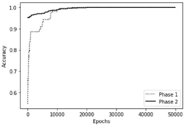
After the two phases of training the model reported an accuracy of 1.0 and a loss of

0.0015. The maximum accuracy of 1.0 is already reached after approximately 20.000 epochs

in both phases. The accuracy of the model during the training is shown in figure 12. After

introducing the new sentences with an embedded clause for phase 2 the accuracy initially

dropped to .93. This is to be expected when new input-output relations are introduced. With

the new data added the accuracy reached 1.0 after approximately 20.000 epochs. The loss kept

decreasing until it reached 0.0017 after 50.000 epochs. This accuracy is considered very high

and may be an indication of overfitting. Overfitting occurs when the model overoptimizes on

the set of training data and learns all the specifics of the training set that cannot be generalized

to other new data (Chollet, 2018). This would lead to less predictive power for the test data.

The input-output relations in the training set are learned to perfection and are therefore classified correctly when fed to the model after training. For every output the activation for

each node ranges between 0 and 1. The correct outputs are produced by the model for the

training set with activation levels above 0.9 and there are no spurious activations (< 0.1). This

is similar to the results by van der Velde & de Kamps (2010). The next step to determine the

performance of the model was to test it with the set of test sentences. These sentences are

[image:27.595.73.402.481.707.2]

based on the training set with different combinations and extensions of the clauses.

(28)

28

5.2 Performance on test data

Evaluation of the fully trained model in Keras gives an accuracy of .99 and a loss of

0.066 for the test data. These results are comparable to the results on the training data and

therefore it seems the model has not overfit. The output activation for each word in the set of

test sentences was evaluated to see the performance in detail.

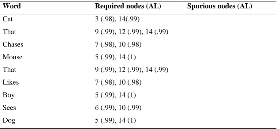
The first sentence in the test set is an extension of a sentence with an embedded clause

in which the theme in a relative clause also has a relative clause. The trained model produced

the correct output for this sentence. Every required output node had an activation higher than

0.9 and the other nodes were all below 0.1 meaning that there was no spurious activation. The

[image:28.595.72.530.352.563.2]

exact activation levels for each input are given in table nine.

Table 9

Activation levels (AL) as given by the model with 12 hidden nodes for the test sentence: Cat that chases mouse that likes boy sees dog.

Word Required nodes (AL) Spurious nodes (AL)

Cat 3 (.98), 14(.99)

That 9 (.99), 12 (.99), 14 (.99)

Chases 7 (.98), 10 (.98)

Mouse 5 (.99), 14 (1)

That 9 (.99), 12 (.99), 14 (.99)

Likes 7 (.98), 10 (.98)

Boy 5 (.99), 14 (1)

Sees 6 (.99), 10 (.99)

Dog 5 (.99), 14 (1)

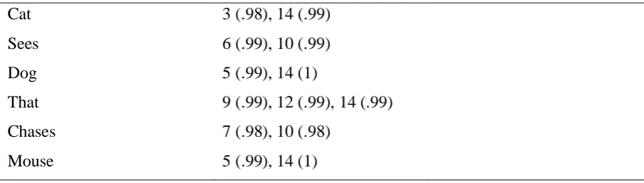
The second sentence in the test set, Cat sees dog that chases mouse, has a subject relative clause in the object position. The model was only trained with subject relative clauses

in the subject position. However, the trained model correctly activated the required nodes with

levels above 0.9 and again no spurious activations as shown in table 10 .

Table10

Activation levels (AL) as given by the model with 12 hidden nodes for the test sentence: Cat sees dog that chases mouse.

(29)

29

Cat 3 (.98), 14 (.99)

Sees 6 (.99), 10 (.99)

Dog 5 (.99), 14 (1)

That 9 (.99), 12 (.99), 14 (.99)

Chases 7 (.98), 10 (.98)

Mouse 5 (.99), 14 (1)

The third sentence in the test set is one with a multiple object-relative clause and is

difficult for humans to understand (van der Velde & de Kamps, 2010). However, the model

was able to correctly activate the required binding categories for all the input-output relations.

[image:29.595.71.524.69.198.2]

There were no spurious activation and all the required activation were above 0.9 as shown in

[image:29.595.71.533.402.612.2]

table 11.

Table 11

Activation levels (AL) as given by the model with 12 hidden nodes for the test sentence: Cat that dog that boy likes sees chases mouse.

Cat 3 (.98), 14(.99)

That 9 (.99), 12 (.99), 14 (.99)

Dog 4 (.99), 13 (.93), 14 (1)

That 9 (.99), 12 (.99), 14 (.99)

Boy 4 (.99), 13 (.93), 14 (1)

Likes 7 (.99), 8 (.98)

Sees 7 (.99), 8 (.98)

Chases 6 (.99), 10 (.99)

Mouse 5 (.99), 14 (1.0)

In table 12 the activation levels for the test sentence, Cat chases mouse that dog that boy likes sees, are given. Again all the required nodes are activated with levels above .9 and there are no spurious activations.

(30)

30

Activation levels (AL) as given by the model with 12 hidden nodes for the test sentence: Cat chases mouse that dog that boy likes sees.

Cat 3 (.98), 14(.99)

Chases 6 (.99), 10 (.99)

Mouse 5 (.99), 14 (1)

That 9 (.99), 12 (.99), 14 (.99)

Dog 4 (.99), 13 (.93), 14 (1)

That 9 (.99), 12 (.99), 14 (.99)

Boy 4 (.99), 13 (.93), 14 (1)

Likes 7 (.99), 8 (.98)

Sees 7 (.99), 8 (.98)

For the test sentence: Fact that cat that boy likes chases mouse worries dog all input-output relations were processed correctly by the trained model. All with activations above 0.9

[image:30.595.69.535.111.322.2]

and without spurious activation as shown in table 13.

Table 13

Activation levels (AL) as given by the model with 12 hidden nodes for the test sentence: Fact that cat that boy likes chases mouse worries dog.

Fact 3 (.99), 11 (.99)

That 9 (.98), 11 (.96), 12 (.98)

Cat 4 (.93), 14 (.99)

That 9 (.99), 12 (.99), 14 (.99)

Boy 4 (.99), 13 (.93), 14 (1)

Likes 7 (.99), 8 (.98)

Chases 7 (.98), 10 (.98)

Mouse 5 (.99), 14 (1)

Worries 6 (.99), 10 (.99)

Dog 5 (.99), 14 (1)

(31)

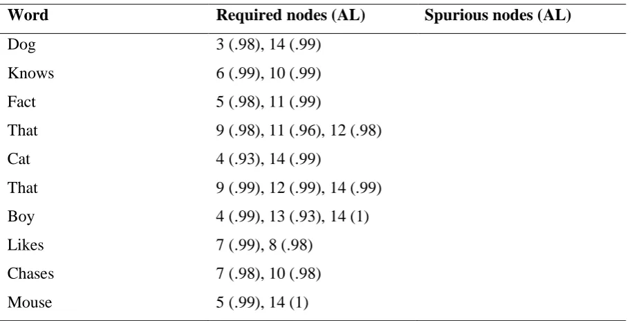
31 binding categories are activated by the trained model. All of the activation are higher than .9

and therefore sufficient to create the appropriate bindings. No other nodes were activated with

[image:31.595.71.535.213.445.2]

a level higher than .1 meaning there is no spurious activation for this sentence structure.

Table 14

Activation levels (AL) as given by the model with 12 hidden nodes for the test sentence: Dog knows fact that cat that boy likes chases mouse.

Dog 3 (.98), 14 (.99)

Knows 6 (.99), 10 (.99)

Fact 5 (.98), 11 (.99)

That 9 (.98), 11 (.96), 12 (.98)

Cat 4 (.93), 14 (.99)

That 9 (.99), 12 (.99), 14 (.99)

Boy 4 (.99), 13 (.93), 14 (1)

Likes 7 (.99), 8 (.98)

Chases 7 (.98), 10 (.98)

Mouse 5 (.99), 14 (1)

In the remaining sentences in the test set there are some outputs that the model did not

activate correctly. For the sentence, Cat who fact that boy likes dog worries chases mouse, an error was made by the model. Firstly, for the verb likes the wrong binding categories were activated. The verb is correctly bound as the verb of a clause (V-v-C). However, the node for theme (T, node 10) is not correctly activated and instead the node for clause as theme of a

verb (V-t-C, node 8) is activated. This In table 15 the activation levels for these nodes is

shown.

Table 15

Activation levels (AL) as given by the model with 12 hidden nodes for the test sentence: Cat who fact that boy likes dog worries chases mouse.

Cat 3 (.98), 14 (.99)

(32)

32

Fact 4 (.99), 11 (.99), 13 (.98)

That 9 (.98), 11 (.96), 12 (.98)

Boy 4 (.99), 13 (.91), 14 (1)

Likes 7 (.99), 10 (.01)* 8 (.98)

Dog 5 (.99), 14 (1)

Worries 7 (.99), 8 (.98)

Chases 6 (.99), 10 (.99)

Mouse 5 (.99), 14 (1)

Note: *AL below threshold of .9.

In the last test sentence of the test set for the verb likes the theme node (T) is not correctly activated. Instead the node for binding a clause word as theme of a verb (V-t-C) is

activated. The activation levels for this sentence are given in table 16. The error made by the

model is the same error as the one that was made in the test sentence shown in table 10. This

shows that the model was not able to learn to activate the desired nodes for these input-output

[image:32.595.73.533.486.714.2]

relations. This result will be discussed more extensively in the discussion section.

Table 16

Activation levels (AL) as given by the model with 12 hidden nodes for the test sentence: Cat chases mouse who fact that boy likes dog worries.

Cat 3 (.98), 14 (.99)

Chases 6 (.99), 10 (.99)

Mouse 5 (.99), 14 (1)

Who 9 (.99), 12 (.99), 14 (.99)

Fact 4 (.99), 11 (.99), 13 (.98)

That 9 (.98), 11 (.96), 12 (.98)

Boy 4 (.93), 14 (.99)

Likes 7 (.99), 10 (.01)* 8 (.98)

Dog 5 (.99), 14 (1)

Worries 7 (.99), 8 (.98)

(33)

33 With the exception of the last two sentences the results of van der Velde and de

Kamps (2010) could be replicated. The first six sentences of the test set are processed without

any problems by the trained model. All of the bindings in these sentences proceed correctly,

under the assumption that the conditional nodes are activated in the NBA.

5.3 Effect of number of nodes in the hidden layer

After these first simulations the configuration of the model was adjusted to study the

effect on the performance. Mainly, the number of hidden nodes was lowered from the initial

twelve to no nodes/hidden layer at all. All other configurations and training steps were kept

the same as the replication with the original model described above. In figure 13 the effect on

the model accuracy is shown. For each number of nodes in the hidden layer the performance

for processing the set of training and test sentences was evaluated. The change in accuracy

across the varying amount of hidden neurons is slightly erratic. With as little as seven hidden

nodes the accuracy of the model for the predicting the test data remains near perfect. It is only

with less than six nodes that the accuracy starts to drop but not in a significant amount. The

accuracy stays well above a level of .96 until a model with only three nodes in the hidden

layer. The model with a hidden layer consisting of one or two hidden nodes has the lowest

accuracy. Even lower than a model that has no hidden layer at all. In fact, the model in which

the hidden layer was completely omitted showed a performance similar to the original model

with a hidden layer consisting of 12 nodes.

(34)

34 The loss, shown in figure 14, shows a similar pattern across the varying hidden layer

sizes. Loss is the highest for the models with one and two hidden nodes. For hidden layer

sizes between seven and twelve the loss remains relatively low. In parallel with the accuracy,

the loss for the model without a hidden layer is similar to that of the original model with

[image:34.595.75.386.180.383.2]

twelve hidden nodes.

Figure 14. Loss shown per model with different number of nodes in the hidden layer.

To investigate the effect of the hidden layer even further all of the test sentences where

processed with the model with zero hidden nodes. The accuracy for this model is just as high

as a model with as many as 12 hidden nodes. This is quite remarkable and therefore all

input-output relations in the test set are examined below. The connection structure of the model

without a hidden layer is shown in figure 12 in the architectures section. This shows that each

input node is directly connected to all nodes in the output layer. The input data thus, does not

pass through a hidden layer first.

In table 17 the first sentence is presented; Cat that chases mouse that likes boy sees dog. All the required nodes are activated with sufficient levels of activation (> .9). However, in two cases there is spurious activation. For chases and likes the eighth node is spuriously activated with a level of .1. This node should only be activated when theword is a clause

word as a theme of a verb. This sentence did not present these difficulties for the original

model with a hidden layer consisting of 12 nodes.

(35)

35

Activation levels (AL) as given by the model with 0 hidden nodes for the test sentence: Cat that chases mouse that likes boy sees dog.

Cat 3 (.95), 14(.99)

That 9 (.98), 12 (.99), 14 (.97)

Chases 7 (.93), 10 (.91) 8 (.10)

Mouse 5 (.99), 14 (.99)

That 9 (.98), 12 (.98), 14 (.96)

Likes 7 (.93), 10 (.91) 8 (.10)

Boy 5 (.99), 14 (.99)

Sees 6 (.98), 10 (.99)

Dog 5 (.99), 14 (.99)

In table 18 the test sentence cat sees dog that chases mouse is presented. Again, for a verb, chases, node eight is spuriously activated. The rest of the binding categories are

[image:35.595.72.533.110.322.2]

activated correctly.

Table 18

Activation levels (AL) as given by the model with 0 hidden nodes for the test sentence: Cat sees dog that chases mouse.

Cat 3 (.95), 14(.99)

Sees 6 (.98), 10 (.99)

Dog 5 (.99), 14 (.99)

That 9 (.98), 12 (.98), 14 (.96)

Chases 7 (.93), 10 (.91) 8 (0.10)

Mouse 5 (.99), 14 (.99)

(36)

36 clause theme. For dog and boy the activation level is .8. additionally, For the two verbs, likes and sees in this test sentence there is an insufficient activation level for node 8.

Table 19

Activation levels (AL) as given by the model with 0 hidden nodes for the test sentence: Cat that dog that boy likes sees chases mouse.

Cat 3 (.95), 14(.99)

That 9 (.98), 12 (.98), 14 (.96)

Dog 4 (.87)*, 13 (.80)*, 14 (.99)

That 9 (.98), 12 (.98), 14 (.96)

Boy 4 (.87)*, 13 (.80)*, 14 (.99)

Likes 7 (.99), 8 (.89)*

Sees 7 (.99), 8 (.89)*

Chases 6 (.98), 10 (.99)

Mouse 5 (.99), 14 (.99)

Note: * AL below the threshold of .9.

As shown in table 20, for the next test sentence the model with no hidden layer makes

the same mistakes as earlier. Namely, the activation levels for nodes 4 and 13 for two noun

inputs are insufficient. And node 8 is not activated adequately for a verb input. The model

[image:36.595.70.538.194.403.2]

with a hidden layer of 12 nodes processed this test sentence without any difficulties.

Table 20

Activation levels (AL) as given by the model with 0 hidden nodes for the test sentence: Cat chases mouse that dog that boy likes sees.

Cat 3 (.95), 14(.99)

Chases 6 (.98), 10 (.99)

Mouse 5 (.99), 14 (.99)

That 9 (.98), 12 (.98), 14 (.96)

Dog 4 (.87)*, 13 (.80)*, 14 (.99)

(37)

37

Boy 4 (.87)*, 13 (.80)*, 14 (.99)

Likes 7 (.99), 8 (.89)*

Sees 7 (.99), 8 (.89)*

Note: *AL below .9.

Activation levels for fact that cat that boy likes chases mouse worries dog are shown in table 21. The model without hidden layer has made several mistakes in processing this sentence. The first occurs at the clause word that. Here, node 11 has an insufficient activation level of .88. The next word in the sentence, cat, is also not processed correctly. Firstly, node 4 has a low activation (.63). Secondly, there is spurious activation for node 3 (AL .15). For the

word boy the same activation levels before are reported. Node 4 and 13 have insufficient activation levels. Lastly, there is a slightly too low activation for node 8 at the verb likes and there is spurious activation for the verb chases.

[image:37.595.75.525.422.655.2]

Table 21

Activation levels (AL) as given by the model with 0 hidden nodes for the test sentence: Cat chases mouse that dog that boy likes sees.

Fact 3 (.95), 11 (.99)

That 9 (.98), 11 (.88)*, 12 (.97)

Cat 4 (.63)*, 14 (.97) 3 (.15)

That 9 (.98), 12 (.98), 14 (.96)

Boy 4 (.87)*, 13 (.80)*, 14 (.99)

Likes 7 (.99), 8 (.89)*

Chases 7 (.93), 10 (.91) 8 (.10)

Mouse 5 (.99), 14 (.99)

Worries 6 (.98), 10 (.99)

Dog 5 (.99), 14 (.99)

Note: *AL below .9.

(38)

38 word in the sentence could be part of a complement clause. However, the activation is

insufficient at a level of .88. the next word cat should then be bound as a noun as the subject of a clause (N-n-C, node 4). This binding fails due to an activation level of .63, which is too

low. Additionally, the node for binding a noun as the subject of a sentence structure is

spuriously activated (AL .15 for node 3). Another two insufficient activations occur at the

noun boy. Node three and 13 are both too low which means boy is not correctly bound as a noun as subject of a clause (N-n-C). Additionally, the clause theme conditional node is not

activated. This would result in a failure to bind the embedded clause cat that boy likes in which boy is the theme of likes. This is also reflected in the fact that at likes the node for binding a word as the theme of a verb (V-t-C) is not sufficiently activated (AL for node 8 =

[image:38.595.72.532.381.611.2]

.89). Lastly, in this sentence structure node 8 is spuriously activated for chases.

Table 22

Activation levels (AL) as given by the model with 0 hidden nodes for the test sentence: Dog knows fact that cat that boy likes chases mouse.

Dog 3 (.95), 14 (.99)

Knows 6 (.98), 10 (.99)

Fact 5 (.98), 11 (.99)

That 9 (.98), 11 (.88)*, 12 (.97)

Cat 4 (.63)*, 14 (.96) 3 (.15)

That 9 (.98), 12 (.98), 14 (.96)

Boy 4 (.87)*, 13 (.80)*, 14 (.99)

8Likes 7 (.99), 8 (.89)*

Chases 7 (.93), 10 (.91) 8 (.10)

Mouse 5 (.99), 14 (.99)

Note: *AL below .9.

In table 23 the activation output for cat who fact that boy likes dog worries chases is shown. This is also the first of the two sentences that was not processed correctly by the

original model with 12 hidden nodes. The activation levels follow a similar pattern to those of

the sentences presented above. There is a combination of activation levels that do not reach

(39)

39 with a too low activation level of .88. At fact a clause theme should also be anticipated with the conditional node CT (node 13). Again, this binding fails.

Table 23

Activation levels (AL) as given by the model with 0 hidden nodes for the test sentence: Cat who fact that boy likes dog worries chases mouse.

Cat 3 (.95), 14 (.99)

Who 9 (.98), 12 (.98), 14 (.96)

Fact 4 (.88)*, 11 (.98), 13 (.87)*

That 9 (.98), 11 (.88)*, 12 (.97)

Boy 4 (.99), 13 (.90), 14 (.96) 5 (.22), 12 (.10)

Likes 7 (.99), 10 (.07)* 8 (.89)

Dog 5 (.99), 14 (.99)

Worries 7 (.99), 8 (.89)*

Chases 6 (.98), 10 (.99)

Mouse 5 (.99), 14 (.99)

Note: *AL below .9.

The activation levels as given by the model with zero hidden nodes for the test

[image:39.595.73.531.194.428.2]

sentence cat chases mouse who fact that boy likes dog worries are given in table 24. At the input word fact the first error occurs. The activation levels for node four and 13 are too low. Another node that is not sufficiently activated is node 11 for the input word that. For boy there is both too little activation and spurious activation. The same counts for the verb likes. Here the same error occurs as with the model with 12 hidden nodes.

Table 24

Activation levels (AL) as given by the model with 0 hidden nodes for the test sentence: Cat chases mouse who fact that boy likes dog worries.

Cat 3 (.95), 14 (.99)

Chases 6 (.98), 10 (.99)

(40)

40

Who 9 (.98), 12 (.98), 14 (.97)

Fact 4 (.88)*, 11 (.98), 13 (.87)*

That 9 (.98), 11 (.88)*, 12 (.97)

Boy 4 (.63)*, 14 (.97) 3 (.15)

Likes 7 (.99), 10 (.07)* 8 (.89)

Dog 5 (.99), 14 (.99)

Worries 7 (.99), 8 (.89)*

Note: *AL below .9.

After reviewing the activation levels for every input-output relation in the test set for

both the model with 12 hidden nodes and the model without a hidden layer, it becomes clear

that the latter is off on way more activations than the former. Where the original model

processed 6 of the 8 test sentences flawlessly, the model without a hidden layer made

mistakes in every sentence. In table 25 some descriptive statistics regarding the models are

presented. The performance of the models is indicated with the number of unsuccessful

bindings and spurious bindings. The model with a hidden layer size of 12 nodes had too low

activation levels for two nodes. On the other hand, the model without a hidden layer made 33 inadequate activations. However, the model without a hidden layer is not the worst

performing model. As can be seen in table 25 and figure 15, the models with ranging from

one to four and the models with six or seven nodes all perform worse. All of these models

have a higher number of failed bindings, more spurious bindings and therefore a lower

proportion correct out of the total activations made. That being said, this analyse paints a

different picture than the accuracy as reported by Keras. The model without a hidden layer is

[image:40.595.71.515.641.767.2]

not capable of flawlessly controlling the binding for the NBA according to these criteria.

Table 25

Overview of the models based on number of failed activations, spurious activations and proportion correct activations.

Model Number of

failed bindings;

AL < .9

Number of spurious

bindings;

AL > .1

Proportion correct

activations out of total

activations

12 hidden nodes 2 2 0.98

(41)

41

2 hidden nodes 170 385 0

1 hidden node 129 417 0.07

No hidden layer 33 12 0.75

[image:41.595.75.461.214.549.2]

Optimization of a control network for binding in combinatorial sentence structures

Optimization of a control network

for binding in combinatorial

sentence structures.

Optimization of a control network for binding in combinatorial

sentence structures.

Abstract

Contents

1. Introduction

2.

Theoretical framework

3. Network architectures

𝑓(𝑥) =

1

1 − ⅇ

4. Method

5. Results