warwick.ac.uk/lib-publications
Manuscript version: Author’s Accepted Manuscript
The version presented in WRAP is the author’s accepted manuscript and may differ from the
published version or Version of Record.
Persistent WRAP URL:
http://wrap.warwick.ac.uk/115036
How to cite:
Please refer to published version for the most recent bibliographic citation information.
If a published version is known of, the repository item page linked to above, will contain
details on accessing it.
Copyright and reuse:
The Warwick Research Archive Portal (WRAP) makes this work by researchers of the
University of Warwick available open access under the following conditions.
Copyright © and all moral rights to the version of the paper presented here belong to the
individual author(s) and/or other copyright owners. To the extent reasonable and
practicable the material made available in WRAP has been checked for eligibility before
being made available.
Copies of full items can be used for personal research or study, educational, or not-for-profit
purposes without prior permission or charge. Provided that the authors, title and full
bibliographic details are credited, a hyperlink and/or URL is given for the original metadata
page and the content is not changed in any way.
Publisher’s statement:
Please refer to the repository item page, publisher’s statement section, for further
information.
G(N, D/N) UP TO GIBBS UNIQUENESS THRESHOLD
CHARILAOS EFTHYMIOU†
Abstract. Approximate randomk-colouring of a graphGis a well studied problem in computer science and statistical physics. It amounts to constructing ak-colouring ofGwhich is distributed close toGibbs distributionin polynomial time. Here, we deal with the problem when the underlying graph is an instance of Erd˝os-R´enyi random graphG(n, d/n), wheredis a sufficiently large constant. We propose a novel efficient algorithm for approximate randomk-colouringG(n, d/n) for any
k≥(1 +)d. To be more specific, with probability at least 1−n−Ω(1) over the input instances
G(n, d/n) and fork≥(1 +)d, the algorithm returns ak-colouring which is distributed within total variation distancen−Ω(1)from the Gibbs distribution of the input graph instance.
The algorithm we propose is neither a MCMC one nor inspired by the message passing algorithms proposed by statistical physicists. Roughly the idea is as follows: Initially we remove sufficiently many edges of the input graph. This results in a “simple graph” which can bek-coloured randomly efficiently. The algorithm colours randomly this simple graph. Then it puts back the removed edges one by one. Every time a new edge is put back the algorithm updates the colouring of the graph so that the colouring remains random.
The performance of the algorithm depends heavily on certain spatial correlation decay properties of the Gibbs distribution.
Key words. Random colouring, sparse random graph, efficient algorithm
AMS subject classifications. Primary 68R99, 68W25,68W20 Secondary: 82B44
∗
Funding:This work is supported by Deutsche Forschungsgemeinschaft (DFG) grant EF 103/11
1. Introduction. LetG=G(n, d/n)denote the random graph on the vertex set
V(G) ={1, . . . , n} where each edge appears independently with probabilityd/n, for a sufficiently large fixed numberd >0.
Approximate randomk-colouring of a graphGis a well studied problem. It amounts to constructing ak-colouring ofGwhich is distributed close toGibbs distribution, i.e. the uniform distribution over all thek-colourings ofG, in polynomial time. Here, we consider the problem when the underlying graph is an instance of Erd˝os-R´enyi random graphG=G(n, d/n). This problem is a rather natural one and it has gathered focus in computer science but also in statistical physics.
From a technical perspective, the main challenge is to deal with the so called
effect of high degree vertices. That is, there is a relative large fluctuation on the degrees in G. E.g. it is elementary to verify that the typical instances of G have maximum degreeΘlog loglognn, while in these instances more than 1−e−O(d)fraction of the vertices have degree in the interval (1±)d. Usually the bounds for sampling k-colourings w.r.t. kare expressed it terms of themaximum degreee.g. [14,4,8,9,11]. However, forGit is natural to have bounds for kexpressed in terms of theexpected degreed, rather than the maximum degree.
The related work on this problem can be divided into two strands. The first one is based on Markov Chain Monte Carlo (MCMC) approach. There, the goal is to prove that some appropriately defined Markov Chain1 over the k-colourings of the
input graph is rapidly mixing. The MCMC approach to the problem is well studied [6,3,12]. The most recent of these works, i.e. [6], shows that the well known Markov chain Glauber block dynamicshas polynomial mixing time for typical instances ofG
as long as the number of colours k≥ 11
2d. This is the lowest bound fork as far as MCMC sampling is concerned.
The second strand has been based on message passing algorithms such asBelief propagation [2], which are closely related to the (non-rigorous) statistical mechanics techniques for the analysis of the random graph colouring problem. These message passing algorithms aim to approximate (conditional) marginals of the Gibbs distri-bution at each vertex . Given the marginals, a colouring can be sampled by choosing a vertex v, assigning it a random colour i according to the marginal distribution, and repeating the procedure with the colour of v fixed to i. Of course, the chal-lenge is to prove that the algorithm does indeed yield sufficiently good estimates of the marginals. In a similar spirit, and subsequently to this work, the authors of [17] propose an approximate random colouring algorithm for G which uses the so-called Weitz’s computational tree approach, from [16], to compute Gibbs marginals for colourings. This algorithms requires at least 3dmany colours for the running time to be polynomial, i.e. O(ns) for somes=s(d)>0.
In this work we obtain a considerable improvement over the best previous results by presenting a novel algorithm that only requires k = (1 +)d colours. The new algorithm does not fall into any of the categories discussed above. Instead, it rests on the following approach: Given the input graph, first remove sufficiently many vertices such that the resulting graph has a “very simple” structure and it can be randomlyk -colouredefficiently. Once we have a random colouring of this, simple, graph we start adding one by one all the edges we have removed in the first place. Each time we put back in the graph an edge weupdatethe colouring so that the new graph remains
(asymptotically) randomly coloured. Once the algorithm has rebuilt the initial graph it returns its colouring.
Perhaps the most challenging part of the algorithm is toupdatethe colouring once we have added an extra edge. The problem can be formulated as follows. Consider two fixed graphs GandG0 such thatV(G) =V(G0) andE(G0) =E(G)∪ {v, u} for
somev, u∈V(G). GivenX, a randomk-colouring ofG, we want to createefficiently
a randomk-colouring of the slightly more complex graphG0. It is easy to show that if the vertices v, u have different colour assignments under X, thenX is a random k-colouring of G0. The interesting case is when X(v) = X(u). Then the algorithm should alter the colour assignment of at least one of the two vertices such that the resulting colouring is random conditional that the assignments ofvanduare different. Here, we use an operation which we call “switching” so as to alter the colouring of only one of the two vertices. Roughly speaking, the switching chooses an appropriately large part ofG, which contains onlyv. Then, it repermutes appropriately the colour classes in this part ofGso as to get the updated colouring.
For presenting our results we use the notion of total variation distance, which is a measure of distance between distributions.
Definition 1. For the distributions νa, νb on [k]V, let ||νa −νb|| denote their total variation distance, i.e.
||νa−νb||= max Ω0⊆[k]V |νa(Ω
0)−ν
b(Ω0)|.
For eachΛ⊆V let||νa−νb||Λ be the total variation distance between the projections
of νa andνb on [k]Λ.
Theorem 2. Let >0 be a fixed number, let dbe sufficiently large number and
fixed k≥(1 +)d. Consider G=G(n, d/n) and let µ the uniform distribution over thek-colouring ofG. Letµˆbe the distribution of the colouring that is returned by our algorithm on inputG.
Letc=
80(1+/4) logd, with probability at least1−n
−c over the input instancesG
it holds that
(1) ||µ−µˆ||=O n−c.
The proof of Theorem2appears in Section6.
The following theorem is for the time complexity of the algorithm, its proof ap-pears in Section6.
Theorem 3. With probability at least1−2n−2/3 over the input instancesG, the
time complexity of the random colouring algorithm isO(n2).
Whether the running time of the algorithm is polynomial or not, depends on certain structural properties of the input graphG. Mainly, these properties require that the “short cycles” of G are disjoint. It will be trivial to distinguish the instances that can be coloured randomly efficiently by our algorithm from those that cannot, see in Section6 for further details.
Remark 1. The region ofkfor which our algorithm operates, coincides with what is conjectured to be the so-called “Uniqueness phase” of the k-colourings of G, e.g. see [18].
v
Fig. 1.“Disagreement graph”.
v
Fig. 2.“switching”.
of the error in the output. The running time and the error of the algorithm here are independent, in the sense that the approximation guarantees do not improve by allowing the algorithm run more steps.
Notation. Given some graphG, we letV(G) andE(G) denote the vertex sets and the edge set, respectively. Also, we let ΩG,k be the set of properk-colourings of G. We denote with small letters of the greek alphabet the colourings inΩG,k, e.g. σ, η, τ. We use capital letters for the random variables which take values over the colourings e.g. X, Y, Z. We denote withσv, X(v) the colour assignment of the vertex v under the colouring σ and X, respectively. Given some σ∈ΩG,k, for every i ∈[k] we let σ−1(i)⊆V(G) be the colour class of colouriunder the colouringσ. Finally, for some integerh >0, we let [h] ={1, . . . , h}.
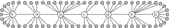
2. Basic Description. So as to give a basic description of our algorithm, we need to introduce few notions. Consider a fixed graph G and let v be a vertex in V(G). Letc, q∈[k] be different with each other and letσbe ak-colouring ofGsuch thatσ(v) =c. We calldisagreement graphQ=Q(G, v, σ, q), the maximal, connected, induced subgraph ofGsuch thatv∈V(Q), whileV(Q)⊆σ−1(c)∪σ−1(q).
Remark 2. The concept of disagreement graph, in the graph theory literature is
also known as Kempe Chain.
In Figure1, the disagreement graphQ(G, v, σ,“green”) is the one with the fat lines. Note thatσspecifies a two colouring for the vertices of Q(G, v, σ,“green”).
Definition 4. ConsiderG,v,σandqas specified above, as well as the disagree-ment graphQ=Q(G, v, σ, q). The “q-switching ofσ” corresponds to the colouring of
Gwhich is derived by exchanging the assignments in the two colour classes inQ.
Figure2illustrates a switching of the colouring in Figure1. That is, the colouring in Figure2differs from the one in Figure1 in that we have exchanged the two colour classes of the subgraph with the fat lines. Theq-switching of any proper colouring of Gis always a proper colouring, too.
We proceed with a high level description of the algorithm. The input is G = G(n, d/n) and some integerk≥(1 +)d. The algorithm is as follows:
Set-up: We construct a sequence of graphs G0, . . . , Gr such thatGris identical to G and Gi is a subgraph of Gi+1. Each Gi is derived by deleting from Gi+1 the edge{vi, ui}. This edge is chosen at random among those which do not belong to a
short cycleofGi+1. We call short, any cycle of length less than (logdn)/9. G0 is the graph we get when there are no other edges to delete.
In above set-up, with probability 1−n−Ω(1), over the instances ofG, the above process generates G0 which is simple2 enough that can be k-coloured randomly in
2In our case,G
G
v u
Fig. 3.“Disagreement graph”.
G
v u
Fig. 4.“switching”.
polynomial time. If G0 is not simple, the algorithm cannot proceed and abandons. Assuming thatG0is simple, the algorithm proceeds as follows:
Update: Take a random colouring of G0. Let Y0 be that colouring. We get Y1, Y2, . . . , Yr, the colourings ofG1, G2, . . . , Gr, respectively, according to the following inductive rule: Given thatGiis colouredYi, so as to getYi+1we distinguish two cases Case (a): Yi (the colouring of Gi) assignsvi and ui different colours, i.e. Yi(vi)6=
Yi(ui)
Case (b): Yi assignsvi andui the same colour, i.e. Yi(vi) =Yi(ui).
In the first case, we setYi+1=Yi, i.e. Gi+1gets the same colouring asGi. In the second case, we chooseq uniformly at random from [k]\{Yi(vi)}, i.e. among all the colours butYi(vi). Then, we setYi+1 equal to theq-switching ofYi. Theq-switching is w.r.t. the graph Gi, the vertex vi and the colouring Yi. The algorithm repeats these steps fori= 0, . . . , r−1. Then it outputsYr.
One could remark that the switching does not necessarily provide ak-colouring where the assignments ofviandui are different. That is, it may be that both vertices vi, ui belong to the disagreement graph in Yi, e.g. Figure 3. Then, after the q-switching the colour assignments of vi and ui remain the same, e.g. Figure 4. It turns out that this situation is rare as long as k= (1 +)d. More specifically, with probability 1−o(n−1), theq-switching ofY
i specifies different colour assignments for vi, ui.
The approximate nature of the algorithm amounts exactly to the fact that on some, rare, occasions the switching somehow fails. The error at the output of the algorithm (see Theorem2) is closely related to the probability of the event that our algorithm encounters such failure when the input is a typical instance ofG.
Remark 3. The lower bound we have for k depends exactly how well we can
control these failures of switching. That is, for k≤dour analysis cannot guarantee that the switching fails only on rare occasions.
3. The setting for the analysis of the algorithm.. Consider a fixed graph Gand letv, ube two distinguished, non-adjacent, vertices.
Definition 5 (Good & Bad colourings).Let σbe a properk-colouring ofG, for
some k > 0. We call σ bad colouring w.r.t. the vertices v, u of G, if σv = σu.
Otherwise, we callσ good.
The idea that underlies the sampling algorithm, reduces the sampling problem to dealing with the following one.
Problem 1. Given abadrandom colouring ofG, w.r.t. {v, u}, turn it to agood
random colouring, in polynomial time.
Consider two differentc, q∈[k] and let Ωc,c and Ωq,c be the set of colourings of G which assign the pair of vertices (v, u) colours (c, c) and (q, c), respectively. Our approach to Problem 1relies on getting a mapping Hc,q :Ωc,c →Ωq,c such that the following holds:
A. IfZ is uniformly random in Ωc,c, then Hc,q(Z) is uniformly random inΩq,c B. The computation ofHc,q(Z) can be accomplished in polynomial time.
It is straightforward that having such a mapping for every two c, q ∈ [k], it is sufficient to solve Problem 1. In the following discussion our focus is on (the more challenging)A. rather thanB.
An ideal (and to a great extent untrue) situation would have been ifΩc,candΩq,c admitted a bijection. Then forA.it would suffice to use forHc,q a bijection between the two sets. Since this is not expected to hold in general, our approach is based on introducing anapproximate bijection between the setsΩc,c andΩq,c. That is, we consider a mapping which is a bijection between two sufficiently large subsets ofΩc,c and Ωq,c, respectively. This would mean that ifZ is uniformly random inΩc,c and Hc,q(·) an approximate bijection betweenΩc,candΩq,c, thenHc,q(Z) isapproximately uniformly random inΩq,c.
To be more specific, we let Hc,q represent the operation of q-switching over the colourings in Ωc,c, as we describe in Section 2. For such mapping, we can find ap-propriateΩc,c0 ⊆Ωc,c andΩq,c0 ⊆Ωq,c0 such thatHc,q is a bijection between the sets Ωc,c\Ω0c,cand Ωq,c\Ω0q,c. We callpathologicaleach colouring σ∈Ω0c,c∪Ω0q,c. For the pathological colouring σ ∈ Ωc,c0 it holds that Hc,q(σ) ∈/ Ωq,c, while for σ ∈ Ωq,c0 it holds thatH−1
c,q(σ)∈/Ωc,c.
Remark 4. There is a natural characterization for the pathological colourings σ ∈ Ωc,c. That is, σ is pathological if the disagreement graph Q = Q(G, v, σ, q)
contains bothv, u.
It turns out that, forZ being uniformly random in Ωc,c, Hc,q(Z) is distributed within total variation distance maxnΩ
0
c,c
Ωc,c,
Ω0q,c Ωq,c
o
from the uniform distribution over Ωq,c. That is, the error we introduce with the approximate bijectionHc,q depends on therelative numberof the pathological colorings inΩc,candΩq,c, respectively. A key ingredient of our analysis is to provide appropriate upper bounds for the two ratios Ω0c,c/Ωc,c, Ω0q,c/Ωq,c.
3.1. Bounding the Error - Spatial Mixing. As in the previous section, let Gbe fixed. For bounding the ratiosΩ0c,c/Ωc,c andΩq,c0 /Ωq,c, we treat both cases in the same way, so let us focus on boundingΩc,c0 /Ωc,c.
It is direct that Ωc,c0 /Ωc,c expresses the probability of getting a pathological colouring if we choose uniformly at random from Ωc,c. For this, consider the si-tuation where we choose u.a.r. fromΩc,c. For every pathP that connectsv, uin the graphG, we letI{P} be an indicator variable which is one if the vertices in the path
P are coloured only with colours c, q in the random colouring and zero otherwise. Equivalently, I{P} = 1 if and only ifP belongs to the graph of disagreement that is
induced by the random colouring and the colourq. It holds that
(2) Ω
0
c,c Ωc,c
= Pr
" X
P
I{P}≥1 #
≤X
P Pr
v a b c d e u
Fig. 5.Boundary at distance 1 from the path.
The first equality follows from the fact that if bothv, ubelong to the disagreement graph, then there should be at least one pathPsuch thatI{P}= 1. The last inequality
follows from the union bound.
Remark 5. The above inequality bounds the relative number of pathological
co-lourings in Ωc,c (resp. in Ωq,c) with the expected number of paths fromv touwhich
are coloured with c, q under a colouring which is chosen at random from Ωc,c (resp. Ωq,c).
In general, computing Pr[I{P}= 1] exactly is a formidable task to accomplish due
to the complex structure we typically have in the underlying graph. For this reason we reside on computing upper bounds of this probability term.
In [5] we used the idea of the so-called “Disagreement percolation” from [1]. The setting of this approach is illustrated in Figure 5, for the path P = (v, a, b, c, d, e, u). The lined vertices are exactly these which are adjacent to the path. So as to bound the probability that the pathP is coloured withc, q, we assume a worst case boundary colouring for the lined vertices. Given the fixed colourings at the boundary, we take a random colouring of the uncoloured vertices in P, conditional v, uare assigned c, and estimate the probability thatP is coloured exclusively withc, q.
Remark 6. The choice of the boundary above, is worst case in the sense that it
maximizes the probability thatI{P}= 1.
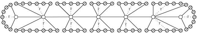
It turns out that considering the worst case boundary condition next to the path P is a too pessimistic assumption. There is an improvement once we adopt a less restrictive approach. The new approach is illustrated in Figure6. Roughly speaking, we consider a worst case boundary condition at the vertices around P which are at graph distancer, forr1. The boundary condition gives rise to Gibbs distribution over the k-colourings of the subgraph confined by the boundary vertices. In parti-cular, we argue about thespatial mixingproperties of the Gibbs distributions in the confined graph. We show that the colouring3of the distant vertices does not bias the
distribution of the colour assignment of the vertices inP by too much.
The above approach is well motivated when we consider G(n, d/n). For such graph, typically, around most of the vertices inP we have a tree-like neighbourhood of maximum degree very close to the expected degree d. This gives rise to study correlation decay for random colourings of a tree with maximum degree∆, for∆≈d. Our spatial mixing results build on the work of Jonasson [10].
3.2. From fixed graph to random graph. When the underlying graphGis fixed, we boundΩc,c0 /Ωc,c (resp. Ωq,c0 /Ωq,c) by using the expected number of paths betweenvanduthat are colouredc, qin a colouring chosen uniformly at random from Ωc,c(resp. Ωq,c). That is, we need to argue on the randomness of thek-colourings of
[image:8.612.109.401.95.144.2]r
r
r
r
r
r
r
r
r
r
r
r
Fig. 6.Boundary at distancerfrom the path
G.
In our analysis, we deal with cases where the underlying graph is random. Then, we have an extra level of randomness to deal with, that of the graph instance. That is, we take an instance of the graph and then, given the graph, we consider a random colouring of this graph instance. Even in this setting, we compute the expected num-ber numnum-ber of paths betweenv anduthat are colouredc, q, however, the expectation is w.r.t. to the randomness of both the graph and its colouring. A result which is central in our analysis is the following one.
Theorem 6. Let >0, let d >0 be sufficiently large and let fixedk≥(1 +)d.
Consider G=G(n, d/n). Let the graphH be such thatV(H) =V(G)andE(H)⊆ E(G). For anyc, q∈[k], different with each other, any non-negative integer`≤log2n
and a permutation P = (w0, . . . , w`)of vertices inV(H)the following is true:
Let X be a randomk-colouring of H conditional than X(w0) =c. Let I{P} = 1,
if P is a path in H andX(wi)∈ {c, q}, for everyj = 1, . . . , `. Otherwise I{P}= 0.
It holds that
(3) Pr[I{P}= 1]≤2[(1 +/4)n]−`.
The proof of the theorem appears in Section9.
Remark 7. In (3) the probability term is w.r.t. both the randomness of H and
the colouring X.
The above theorem implies that for k ≥ (1 +)d, in a random k-colouring of
G, typically, there are not long paths coloured with only two colours. Furthermore, this property is monotone in the graph structure. That is, it holds even though if we remove an arbitrary number of edges fromG(and getH). The monotonicity property follows from the fact that we can extend in a natural way the Gibbs uniqueness condition in [10] from ∆regular trees to trees of maximum degree∆.
4. Updating Colourings. In this section, we describe the process that the random colouring algorithm uses to update the colourings, we call it Update. For the sake of clarity in this section we assume a fixed graphGand we distinguish two verticesv, u∈V(G). We takeksufficiently large so thatGisk-colourable.
Definition 7 (Disagreement graph). For anyσ∈ΩG,k andq∈[k]\{σv}we let
the disagreement graph Q=Q(G, v, σ, q)be the maximal induced subgraph of Gsuch that
V(Q) =
x∈V(G)
∃ path w1, . . . , w`, inGsuch that: w1=v, w`=x, σ(wj)∈ {σv, q},∀j∈[`]
.
[image:9.612.94.416.94.149.2]Switching
Input: G, v, σandq∈[k]\{σv}
setc=σv
setQ=Q(G, v, σ, q)
setτ(V(G)\V(Q)) =σ(V(G)\V(Q))
forw∈V(Q)∩σ−1(c)do
setτ(w) =q
forw∈V(Q)∩σ−1(q)do
setτ(w) =c Output: τ
Switchinghas the following property, whose proof is easy to derive.
Lemma 8. If τ = Switching(G, v, σ, q), where σ ∈ ΩG,k and q 6= σ(v), then τ∈ΩG,k.
The proof of Lemma8, is quite straightforward and appears in Section13.1.
As far the time complexity ofSwitchingis regarded we have the following lemma, whose proof appears in Section13.2.
Lemma 9. For every v∈V(G), anyσ∈ΩG,k,q∈[k]\{σv} the time complexity
of computingSwitching(G, v, σ, q)isO(|E(G)|).
In what follows, we have the pseudo-code forUpdate.
Update
Input: G, v, u, σ∈ΩG,k
if σis a goodcolouring w.r.t. v, u,then setτ=σ
else do
choosequ.a.r. from [k]\{σv}
setτ=Switching(G, v, σ, q) Output: τ
To this end, we need argue about the time complexity and the accuracy ofUpdate. As far as the time complexity is regarded we have the following theorem.
Theorem 10. For anyv, u∈V,σ∈ΩG,k andq∈[k]\ {σv}, the time complexity
of Update(G, v, u, σ, k)isO(|E(G)|).
Theorem10follows as a corollary of Lemma9, once we note that the execution time ofUpdateis dominated by the calls ofSwitching.
So as to study the accuracy of Updatewe introduce the following concepts. For any two different coloursc, qwe letSq(c, c)⊆Ω(c, c) andSc(q, c)⊆Ω(q, c) be defined as follows: The set Sq(c, c) (resp. Sc(q, c)) contains every σ ∈ Ω(c, c) (resp. σ ∈ Ω(q, c)) such that there is no path betweenv and uwhich is coloured only with the coloursc, q, byσ.
Definition 11. Let α = αG,k ∈ [0,1] be the minimum number such that the
Theorem 12. Let ν be the uniform distribution over thek-colourings ofGwhich
aregood, w.r.t. v, u. Let, also,ν0 be the distribution of the output ofUpdatewhen the input colouring is distributed uniformly at random over thek-colourings ofG. Letting
αbe as in Definition11, it holds that
||ν−ν0|| ≤α.
The proof of Theorem12appears in Section12.
5. Random Colouring Algorithm. In this section, we study the time com-plexity and the accuracy of the random colouring algorithm. For the sake of defini-tiveness we assume the input graphGto be fixed and is such thatGisk-colourable. Given the input graphG, the algorithm creates the sequence of subgraphsG0, . . . , Gr. The variable Yi denotes the k-colouring that the algorithm assigns to the graph Gi. Gi is derived by deleting fromGi+1an edge which we call{vi, ui}.
As we consider a general graph G, in the pseudo-code that follows, we do not specify exactly how do we get Gi from Gi+1, i.e. what is {vi, ui}. Also, we do not specify how do we getY0, the random colouring ofG0. We get specific on these two matters only when we considerG(n, d/n) at the input, see Section 6.
The pseudo-code for the algorithm is as follows:
Random Colouring Algorithm
Input: G,k
computeG0, G1. . . , Gr
computeY0 /∗Get a random k-colouring ofG0∗/
for0≤i≤r−1do
setYi+1 the output ofUpdate(Gi, vi, ui, Yi, k) Output: Yr
Using Theorem10and noting thatr≤ |E(G)|, we get the following result.
Theorem 13. Let T(n) be the time complexity for k-colouring randomly G0. Then, the random colouring algorithm has time complexity O(|E(G)|2+T(n)). Next, we investigate the accuracy of the algorithm. For any c, q∈[k] we letΩi(c, q) be the set of colourings ofGi which assign the colourscandq to the verticesvi and ui, respectively. Furthermore, for two different coloursc, q∈[k], letSqi(c, c)⊆Ωi(c, c) andSi
c(q, c)⊆Ωi(q, c) be defined as follows: The setSqi(c, c) (resp. Sci(q, c)) contains every σ∈Ωi(c, c) (resp. σ∈Ωi(q, c)) such that there is no path between vi and ui (inGi) which is coloured byσusing the coloursc, q, only.
Definition 14. For everyi= 0, . . . , r−1, letαi∈[0,1]be the minimum number
such that the following holds: For any pair of different colours c, q the sets Si q(c, c)
and Sci(q, c) contain all but an αi-fraction of the colourings in Ωi(c, c) andΩi(q, c),
respectively.
Clearly the quantitiesαi depend onGi andk.
Theorem 15. Letµbe the uniform distribution over thek-colourings of the input
graph G. Letµˆ be the distribution of the colourings at the output of the algorithm. It holds that
||µ−µˆ|| ≤ r−1
X
i=0 αi,
The proof of Theorem15appears in Section13.3.
6. Random Colouring G(n, d/n). In this section, we focus on the case where the input ofRandom Colouring AlgorithmisG=G(n, d/n). This study leads to the proof of Theorems2 and3.
We start by describing how do we get G0, . . . , Gr from G. LetE(G) ⊆ E(G) contain exactly every edgee∈E(G) such that the shortest simple cycle that contains eis of length greater than (logdn)/9.
ComputingG0, . . . , Gr: The sequenceG0, . . . , Gr is constructed as follows: Set r=|E|+ 1. We setGr=G. GivenGi we getGi−1 by removing a randomly chosen edge ofGi which also belongs to E(G), fori= 1, . . . , r. G0 contains only the edges of the initial graph which do not belong toE(G).
Perhaps it is interesting to describe what motivates the above construction of the sequenceG0, . . . , Gr. Since eachαidepends onGi, we construct the sequence so as to haveP
iαi, as small as possible. The smaller the probability the algorithm encounters a disagreement graph which includes bothvi, uithe smallerαis get. Choosingviand uito be at large distance reduces the probability that the disagreement graph includes both of them, consequently,αi gets smaller. Our choice of sequence forcesvi andui to be at distance greater than (logdn)/9 with each other. To a certain extent, this allows to control the error of the algorithm, i.e. P
iαi.
Given the sequence G0, . . . , Gr, the next step is to argue on how can we get a randomk-colouring ofG0, efficiently. Our arguments rely on the fact that typically G0has a very simple structure, i.e. we use the following result.
Lemma 16. For d > 0, let Sn,d be the set of all graph on n vertices such that
their component structure is as follows: Each component is either the trivial4, or it is a simple isolated cycle5 of maximum length(log
dn)/9. ConsiderGand the sequence G0, . . . Gr created as we described above. It holds that
Pr[G0∈Sn,d]≥1−n−2/3.
The proof of Lemma16appears in Section13.4.
ForG0∈Sn,d,exactrandomk-colouring can be implemented efficiently. In what follows we describe an efficient process that can colour randomly any graph inSn,d.
Random Colouring in Sn,d
Input: G∈Sn,d,k.
setC to be the set of all cycles inG
foreach isolated vertexv∈V(G)do /*Colour isolated vertices*/
setτ(v) a colour chosen uniformly random from [k]
foreachC= (w0, . . . wl)∈ C do /*Colour isolated cycles*/
setτ(w0) a color chosen uniformly random from [k]
fori= 1, . . . , ldo
setµwi the Gibbs marginal of wi, conditional τ(w0), . . . , τ(wi−1) computeµwi using Dynamic Programming
setτ(wi) according toµwi
Output: τ
4single isolated vertex
The most interesting part of the above algorithm is the one for random colouring of the cycles. For each cycle C ∈ C, the algorithm first assigns a random colour on the vertexw0. Oncew0is assigned a colour, then we eliminate the cycle structure of C and now we deal with a tree of maximum degree 2. This allows to compute the marginalµwi, for each vertexwi∈C, by usingDynamic Programming (DP).
Remark 8. The use of DP for computing Gibbs marginals on the trees is well
known to be exact, e.g. see [15] for an excellent survey on the subject.
Remark 9. The recursive distributional equations that DP uses in this setting
are more or less standard. Example of such equations appear in the proof of Lemma
25, in Section 11.1.
Once we get an exact random colouring of G0 by using the above algorithm,
Random Colouring Algorithm colours the remaining graphs G1, . . . , Gr by using
Update, as we described in Section5.
LetXn,dcontain every graphGonnvertices such that the following holds: 1. getting a sequence of subgraphsG0, . . . , Gr, as described in Section6, it holds
thatG0∈Sn,d
2. |E(G)| ≤(1 +n−1/3)dn/2.
Note that for someGwe have thatG0∈Sn,d regardless of the order we remove the edges for creating the sequence G0, . . . , Gr. That is, whetherG ∈Xn,d, or not, depends only on the graphG.
If the input graph G does not belong into Xn,d, then the Random Colouring
Algorithmabandons. It turns out that this typically does not happen. In particular, we have following corollary.
Corollary 17. For sufficiently large d > 0, it holds that Pr[G ∈ Xn,d] ≥1− 2n−2/3.
Proof. Lemma 16, states that for the sequenceG0, . . . , Gr generated fromG as described in Section 6 it holds that Pr[G0 ∈ Sn,d] ≥ 1−n−2/3. Using Chernoff’s bounds, e.g. [13], we also get
Prh|E(G)| ≥(1 +n−1/3)dn/2i≤exp−n1/4.
A simple union bound, yields that indeed Pr[G∈Xn,d]≥1−2n−2/3. In the following two sections we prove Theorems2and3.
6.1. Proof of Theorem2. For proving Theorem2we need to use the following result, whose proof appears in Section7.
Theorem 18. Let , d, k be as in the statement of Theorem 2. Consider the
sequenceG0, . . . , Grgenerated fromGas described in Section6. Fori∈ {0, . . . , r−1}
it holds that
E[αi]≤50−1k(4 +)n
−(1+
36(1+/4) logd).
Proof of Theorem 2. In light of Corollary 17, it suffices to show that (1) holds with sufficiently large probability over the instancesG, conditional thatG∈Xn,d.
Let A be the event G ∈ Xn,d. First we argue about E[||µ−µˆ|| | A], i.e. the
expectation is w.r.t. the instances G. Using Theorem 15 and Theorem18 we have that
E[||µ−µˆ|| | A]≤E
"r−1 X
i=0 αi | A
#
where the expectation is taken over the instancesG. Noting thatαi ∈[0,1], we get
(4) E[||µ−µ0|| | A]≤
(1+n−1/3)dn/2
X
i=0
E[αi | A],
where the above follows by observing thatAimplies thatr≤(1 +n−1/3)dn/2. On the other hand for the quantitiesE[αi | A] we work as follows:
E[αi | A]≤(Pr[A])− 1
·E[αi] [sinceαi≥0]
≤100−1k(4 +)n−(1+
36(1+/4) logd),
(5)
in the final inequality we used Theorem18 and Corollary17. Plugging (5) into (4), we get that
E[||µ−µˆ|| | A]≤C·n−
36(1+/4) logd,
for fixedC >0. The theorem follows by applying Markov’s inequality.
6.2. Proof of Theorem3. First, we are going to show that, on inputG∈Xn,d,
Random Colouring Algorithm has time complexity O(n2). Then, the theorem will follow by using Corollary17.
We start by considering the time complexity of the algorithm on inputG∈Xn,d. First the algorithm constructsG0, . . . , Gr. For this, it needs to distinguish which edges inE(G) do not belong to a short cycle. This can be done by exploring the structure of the (logdn)/9-neighbourhood around each edge of G by usingBreadth First Search (BFS). The search around each edge requiresO(n) steps, since|E(G)|=O(n). The exploration is repeated for each edge in E(G). Thus, the algorithm requiresO(n2) steps to find the short cycles. This implies that G0, . . . , Gr can be constructed in O(n2) steps.
Since the |E(Gi)| = O(n), for every i = 0, . . . , r, Theorem 10 implies that the number of steps required for eachUpdatecall is O(n). Consequently, we needO(n2) steps for all the calls ofUpdate, sincer≤ |E(G)|=O(n).
It remains to consider the time complexity of colouring randomlyG0. The algo-rithms uses Random Colouring inSn,d (Section 6) to colour randomly G0. Due to
our assumptions it holds thatG0∈Sn,d. LetCbe the set of cycles inG0. Note that all the cycles in C are simple and isolated from each other. Also, all the vertices in G0which are not in a cycle are isolated.
We consider the time complexity of colouring the cycles in C. For each C = (w0, . . . , w|C|)∈ C, first, the problem is reduced to computing Gibbs marginals on a
tree of maximum degree 2. This is done by assigning w0 a uniformly random colour from [k]. Then, the algorithm colours iteratively the vertices inC. At iterationi, the colouring of the verticesw1, . . . , wi−1 is already known and the algorithm colourswi as follows: It computes the marginal µwi, conditional the colour assignment of the
vertices w0, . . . , wi−1, by using Dynamic Programming. Then it assigns a colour to
wi according toµwi.
Given the distribution of the children of wi w.r.t. the subtree that hangs from them, the Dynamic Program requires O(k2) arithmetic operations to compute µ
wi.
This means that the algorithm requiresO(k2|C|) operations for computingµ
wi. It is
clear that each cycleCrequires at most O(k2|C|2) steps to be coloured randomly. Consequently, the algorithm requires O(k2nlog2
Concluding, the time complexity of Random Colouring inSn,d, for fixed k is
O(nlog2n). This implies that Random Colouring Algorithm, on input G ∈ En,d, has time complexityO(n2).
The theorem follows.
7. Proof of Theorem18. LetΛn,kdenote the set of all the 4-tuples (G, v, u, σ) such thatGis a kcolourable graph onnvertices,v, u∈V(G) andσis ak-colouring of G. For (G, v, u, σ) ∈ Λn,k and q ∈ [k]\{σv}, consider the disagreement graph
Q=Q(G, v, σ, q) and let the eventQσv,q= “u∈Q”.
Forc1, c2∈[k] and an integeri≥0 we let the distributionPi
c1,c2over (G, v, u, Z)∈ Λn,k be induced by the following experiment: Take an instanceG and construct the sequenceG0, . . . , Gr as described in Section6. Then,
1. Gis equal toGi
2. v anduare equal tovi andui, respectively 3. Z is distributed uniformly at random inΩG(c1, c2)
Remark 10. In G0, . . . , Gr, the number of terms in the sequence is a random
variable. In the definition of Pi
c1,c2 if i > r we follow the convention that G is the
empty graph with probability1.
Also, denote byPi
∗,c2 the distribution whenZ(v) is not fixed, i.e. Z is a random k-colouring of G, conditional thatZ(u) = c2. In the same manner, denote byPi
c1,∗,
the distribution when Z(u) is not fixed. Finally, we define Pi
∗,∗ when there is no
restriction on the colouring of bothv, u.
For proving Theorem18we need the following two results.
Proposition 19. Let , d and k be as in the statement of Theorem 18. Let
c, q∈[k]be such thatc6=q. For anyi≥0, it holds that
Pi
c,∗[Qc,q]≤10−1(4 +)n
−(1+
36(1+/4) logd).
The proof of Proposition19appears in Section8.
Lemma 20. Let , d, k be as in the statement of Theorem 18. For any c ∈ [k]
and any i≥0 it holds that
||Pi
c,∗(·)− P∗i,∗(·)||{ui} ≤n −1.
The proof of Lemma20appears in Section7.1.
Proof of Theorem 18. It is elementary to verify that
(6) E[αi]≤ max
c,q∈[k]:c6=q
Pi
c,c[Qc,q] +Pq,ci [Qq,c] .
The theorem follows by bounding appropriately the probability terms in the r.h.s. of (6).
Given (G, v, u, σ)∈Λn,k, we let the eventsE:=“σ(v) =σ(u)” andAc1 :=“σ(u) = c1”, for every c1 ∈ [k]. Since it holds that Pc,i∗[Qc,q] ≥ Pc,i∗[Qc,q|E]· Pc,i∗[E] and
Pi
c,∗[·|E] =Pc,ci [·], we get that
(7) Pi
c,c[Qc,q]≤ 1 Pi
c,∗[E]
Noting thatPi
c,∗[E] =Pc,i∗[Ac] andP∗i,∗[Ac] =k−1, from Lemma20we get that
(8)
Pc,i∗[E]−k−1 ≤n−1.
Using (8) and (7) we get that
(9) Pi
c,c[Qc,q]≤2k· P i
c,∗[Qc,q]≤20−1k(4 +)n
−(1+
36(1+/4) logd),
where the last inequality follows from Proposition19. Applying the same arguments we, also, get that
(10) Pi
q,c[Qq,c]≤20−1k(4 +)n−(
1+
36(1+/4) logd).
The bounds in (9) and (10) hold for any c, q ∈ [k], different with each other. The theorem follows by plugging (9) and (10) into (6).
7.1. Proof of Lemma 20. Let (G, v, u, X),(G, v, u, Z)∈ Λn,k, for some fixed G. LetX, Z be two coupled random colourings ofG. In particular forX, Z we have the following: Assuming that X(v) = c, we choose q u.a.r. among [k] and we set Z(v) =q. Depending on whetherc=qor not the coupling does the following choices. Case “c=q”: CoupleZ andX identically, i.e. X =Z
Case “c6=q”: SetZ=Switching(G, v, X, q),
where Switchingis from Section 4. Claim 1 establishes that Z follows the ap-propriate distribution.
Claim 1. Switching(G, v, X, q)is a random colouring of Gconditional on that
v is colouredq.
Proof. It suffices to show that Ωc = ∪c0∈[k]Ωi(c, c0) and Ωq = ∪c0∈[k]Ωi(q, c0) admit the bijectionSwitching(G, v,·, q) :Ωc→Ωq.
First, note that Lemma 8 implies that if τ = Switching(G, v, σ, q), then τ ∈ ΩG,k. Also, it is direct that τ ∈ Ωq. Second, we need to show that the mapping
Switching(G, v,·, q) : Ωc → Ωq is surjective, i.e. for any σ ∈Ωq there is aσ0 ∈Ωc such thatσ =Switching(G, v, σ0, q). Clearly, suchσ0 exists. In particular, it holds
that σ0 =Switching(G, v, σ, c). The last observation also implies that the mapping
isone-to-one. SinceSwitching(G, v,·, c) is surjective and one-to-one it is a bijection. The claim follows.
For the case where q 6= c, consider the disagreement graph Q =Q(G, v, X, q). We remind the reader that the event Qc,q :=“u∈Q”. Due to the way we construct Z we have that the eventQc,q holds if and only ifX(u)6=Z(u) holds. That is,
(11) Pr[X(u)6=Z(u)]≤Pr[Qc,q].
Note that the probability terms above hold for anyk-colourable graphG.
For our purpose, we need to consider (G, v, u, X),(G, v, u, Z) distributed as in Pi
c,∗ andPq,i∗ respectively, forq6=c. For such 4-tuples, (11) implies that
Pr[X(u)6=Z(u)]≤ Pc,i∗[Qc,q].
Note that the above is derived by taking averages w.r.t. the graph instanceGi in the sequenceG0, . . . , Grwhere (v, u) correspond to (vi, ui). The lemma follows by noting that
||Pc,i∗(·)− P
i
∗,∗(·)||{u}≤ Pc,i∗[Qc,q], while from Proposition19we have thatPi
8. Proof of Proposition 19. Let (G, v, u, X) be distributed as inPi
c,∗. Every
pathP in Gwhich start from v and∀w∈P we haveX(w)∈ {c, q} is calledpath of disagreement. It holds that
Pi
c,∗[Qc,q]≤ Pc,i∗[B] +Pc,i∗[C],
where the eventsB andCare as follows: B:=“vanduare connected through a path of disagreement of length at most log2n”. C :=“v and uare connected through a path of length greater than log2n’.
Let, also, the eventC0 := “there is a path of disagreement starting fromvand has length greater than log2n”. Note that the event C0 does not specify the end vertex
of the path of disagreement. It is immediate thatPi
c,∗[C0]≥ Pc,i∗[C], since, the event
C is included in the eventC0. Thus, it holds that
Pi
c,∗[Qc,q]≤ Pc,i∗[B] +Pc,i∗[C0].
The proposition will follow by bounding appropriately the probabilities Pi c,∗[B]
andPi c,∗[C0].
For every vertex w, we letΓw(l) denote the number of paths of disagreement of lengthlthat connect vandw. From Markov’s inequality we get that
(12) Pc,i∗[B]≤EPi c,∗
X
l≤log2n Γu(l)
,
where EPi
c,∗[·] is the expectation w.r.t. Pic,∗. For bounding P
i
c,∗[C0] we use the
following inequality
(13) Pi
c,∗[C0]≤EPi c,∗
" X
w
Γw(log2n)
#
,
where the summation on the r.h.s. of the inequality, above, runs over all the vertices of the graph.
So as to compute the expectation both in (12) and (13) we use Theorem 6. However, we note that the pair of verticesv, uwe consider is not a uniformly random one. Since we consider the probability distribution Pi
c,∗, the pair v, u is distributed
uniformly at random among the pair of vertices which are at distance greater than (logdn)/9 inG.
Lettingpbe the probability that a randomly chosen edge fromGdoes not belong to a cycle of length less than (logdn)/9. Using Theorem6we get that
(14)
EPi c,∗
X
l≤log2n Γu(l)
≤2p−
1 log2n
X
l≥l0
nl−1((1 +/4)n)−l, forl0= (logdn)/9 + 1.
probability of each of these paths to be disagreeing is 2 ((1 +/4)n)−l. We divide by p due to conditioning that the vertices v, u are not entirely random, since we have conditioned that their distance is larger than (logdn)/9.
It is direct to show that it holds thatp≥1−n−9/10. Then, we have that
(15) EPi
c,∗
X
l≤log2n Γu(l)
≤4−
1(4 +)n−1−
36(1+/4) logd.
Working in the same manner for (13) we get that
EPi c,∗
" X
w
Γw(log2n)
#
≤2p−1(1 +/4)−log2n
≤2p−1n−((logn)·log(1+/4))≤n−√logn, (16)
where the last inequality holds for largen and noting thatp >1/2. Observe that in the second case the number of paths of lengthl that emanate fromv is at most nl, as we do not fix the last vertex of the path.
Using (15) and (12) we bound appropriately Pi
c,∗[B]. Using (16) and (13) we
bound appropriatelyPi
c,∗[C0]. The proposition follows.
9. Proof of Theorem6. For the sake of brevity we denote withP not only the permutation of the verticesw0, . . . , w` but the corresponding path inH, if such path exists. The probability term in (3) is w.r.t. both the randomness of the graph H
and the randomk-colourings ofH. That is, for I{P}= 1, first we need to have that
the vertices in the permutationP form path inH. Then, given thatH contains the path P, we need to bound the probability that this path is 2-coloured in a random k-colouring ofH. Clearly, the challenging part is the second one. We denoteHP the graphH conditional that the pathP appears in the graph.
Our approach is as follows: GivenHP, first we specify an appropriate subgraph ofHP which includes the pathP. We call this subgraphN. Also, we specify a set
B⊂V(N) such that B separatesV(N)\B from the rest of the graphHP. We set an appropriate (worst case) boundary condition σB ∈ [k]B on B. Let µσN, be the Gibbs distribution of thek-colourings ofN, conditional thatB is colouredσB. The choice of σ is such that underµσN the probability of P to be 2-coloured with c, q is lower bounded by the corresponding probability underµH, the Gibbs distribution of thek-colourings ofHP.
Let us describe how do we getN andB⊂V(N). For this, we consider an integer parameterh= h() >0, which we assume that is sufficiently large it depends on and it is independent ofd.
Path Neighbourhood Revealing. Consider the graph HP. For eachwi ∈P we define the sets Li,s ⊆ V(HP), for s = 0, . . . , h, as follows: Li,0 = {wi}. We get Li,s by working inductively, i.e. we use Li,s−1. Let Ri,s ⊂ V(G) contain all
the vertices but those which belong toP and those which belong inS
j<i
S
j0≤hLj,j0 and S
j0<sLi,j0. Consider an (arbitrary) ordering of the vertices in Ri,s. For each vertexu∈Li,s−1 we examine its adjacency with the vertices inRi,sin the predefined order. We stop revealing the neighborhood ofuinRi,s once we either have revealed (1 +/3)d+ 1 many neighbours, or if we have checked all the possible adjacencies of u with Ri,s. Whichever happens first6. Then L
i,s contains all the vertices in Ri,s
6Clearly, as the process goes, the number of neighbours ofuinR
h
h
h
h
h
h
h
h
Fig. 7.The lined vertices belong toB.
which have been revealed to have a neighbour inLi,s−1.
Fori= 0, . . . , `, letNi,hbe the induced subgraph ofHP with vertex setS h s=0Li,s. Note that the size of Ni,h depends only on , d, h, i.e. it is independent of n. In particular, it holds that
(17) |V(Ni,h)| ≤N0=
[(1 +/3)d+ 1]h+1−1 (1 +/3)d .
We callNi,h,Failif at least one of the following happens: • The maximum degree inNi,h is at least (1 +/3)d+ 1 • The graphNi,h is not a tree
• There is an integerj6=isuch that some vertexw00∈Nj,his adjacent to some vertexw0 ∈ Ni,h and the edge{w0, w00}does not belong to the pathP.
Lemma 21. Let, dbe as in Theorem6. Consider a sufficiently large fixed integer h=h()>0, independent of d. Let F be the number of vertices wi ∈ P such that Ni,h isFail, for i= 1, . . . , `. For anys= 1, . . . , `, it holds that
Pr[F =s]≤(1 +n−1/3)
`
s
exp
−2ds/35
.
In the lemma, above,F does not considerN0,h. The proof of Lemma21appears in Section9.1.
The graphN we are looking for is a subgraph ofS`
i=0Ni,h. For specifyingN perhaps it is more natural to start with the set B which separates N from the rest of HP. Each time, we decide onB∩V(Ni,h) by examining each Ni,h, separately. If Ni,his
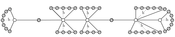
Fail, then B∩V(Ni,h) = {wi}, i.e the vertex in the path P. On the other hand, ifNi,h is notFail, thenB∩V(Ni,h) =Li,h, i.e. all the vertices inNi,h that are at distancehfromwi.
In Figure 7, we see one example of a possible outcome of the exploration we describe above. The lined vertices are exactly those which belong to the boundary set B. If some vertex wi on the path is lined, this means that Ni,h is Fail. The vertices of the path which are not lined correspond to the roots of a “low degree” tree of height at mosth.
Let S ⊆ {0, . . . , `} contain each i such that Ni,h is not Fail. Also, let VA =
S
i∈SV(Ni,h−1) 7. It is not hard to see that the vertex set B is a cut-set that
separates VA from the rest of the vertices in V(HP). The graphN is the induced subgraph ofHP with vertex setVA∪B.
Remark 11. Since HP is random, the subgraph N is random.
7N
[image:19.612.106.404.86.149.2]Consider the graph HP and the corresponding Gibbs distribution µH. The di-stribution µH specifies a convex combination of boundary conditions on B. Using these boundary conditions we could estimate the probability thatP is coloured only with c, q, exactly. However, estimating this convex combination of boundaries is a formidable task to accomplish. We get an upper bound of this probability by consi-dering a worst boundary condition on the vertex setB. The condition is worst in the sense that it maximizes the probability of interest. That is, instead ofµH, we consider the distributionµσN which is much easier to handle. Under µσN the probability that P is coloured withc, qis at least as big as underµH.
In the following results, we let Td,,h be the set of labeled, rooted, trees of maxi-mum degree (1 +/3)dand height h.
Proposition 22. Let , d, k be as in Theorem 6. Consider a sufficiently large
fixed integer h = h() > 0, independent of d. Consider HP and let N,B be as
defined above. For each wj ∈P such thatwj∈/ B the following is true:
Let Γ be the neighbours of wj in the path P and let B+ =B∪Γ. There exists
a functionf :N→R+, such that f(h)→0 ash→ ∞, while for anyσ∈ΩN,k and
any c∈[k]it holds that
max Nj,h
|Pr[X(vj) =c |Nj,h, XB+=σB+]−Pr[X(vj) =c |Nj,h, XΓ =σΓ]| ≤ f(h)
k ,
where the maximum is over all Nj,h∈ Td,,h andX is a randomk-colouring of N. Note that the above is a spatial mixing result. It implies that for anyNj,hwhich is notFailthe boundary we set at distancehfromwjhas small effect on the distribution of thek-colouring ofwi. The proof of Proposition 22appears in Section 10.
For everywj ∈P such that wj∈B, the worst case boundary condition sets the vertex to its appropriate colour, i.e. if j is even then the colour is c, otherwise the colour is q. Proposition 22 implies that, whatever is the boundary condition at B, if wj ∈/ B, its probability of getting colour q or c, depending on the parity of j, is approximately 1/k.
Proof of Theorem 6. LetEP be the event thatH contains the pathP. It holds that
Pr
I{P}= 1≤(d/n)
` ·Pr
I{P}= 1|EP.
ConsiderHP and letX be a randomk-colouring conditional on thatX(w0) =c. For i even, we callwi ∈P disagreeing ifX(wi) =c. For i odd number, we call wi ∈P disagreeing ifX(wi) =q.
Let the eventDi that “wi is disagreeing”. Clearly it holds that
(18) Pr
I{P}= 1
≤(d/n)`Pr
∩`
i=1Di |EP
.
Let the events Ai, Bi, Ci be defined as follows: Ai = “Ni,h is Fail”. Bi = “Ni,h is notFailandwi is disagreeing”. Also letCi=Ai∪Bi.
Claim 2. It holds that
Pr
∩`
i=1Di |EP
≤Pr
∩`
i=1Ci | EP
.
Proof. In the setting of the proof of Theorem 6, assume that we have revealed the underlying graphHP. It suffices to show that
(19) Pr
∩` i=1Di
HP
≤Pr
∩` i=1Ci
HP
Observe that the probability terms are only w.r.t. the random colouring ofHP. LetW be the set of verticesqi∈P such thatNi,his not Fail. Also, letW0⊆B be the set of vertices wi ∈ P for which Ni,h is Fail. The events ∩wi∈WCi and
∩wi∈WDi are identical, since both occur if the vertices inW are disagreeing. Thus it holds that Pr [∩wi∈WDi | HP] = Pr [∩wi∈WCi | HP].
Furthermore, we note that Pr [∩wi∈W0Ci | HP,∩w
i∈WCi] = 1. On the other
hand, it holds that Pr [∩wi∈W0Di| HP,∩w
i∈WDi] ≤ 1. These imply that (19) is
true. The claim follows.
Using Claim2and (18), it suffices to bound appropriately Pr
∩`
i=1Ci | EP.
ConsiderHP and letFi(C) be theσ-algebra generated by the eventsCj, for every j6=i. Proposition22implies that
(20) ρ= Pr[Bi | Fi(C), EP, Ni,h is notFail]≤(k−2)−1+f(h)/k.
for any i = 0, . . . , `. LettingF be the number of vertices wi ∈ P such that Ni,h is
Fail, fori= 1, . . . , `, we have that
Pr
∩`i=1Ci |EP
= `
X
s=0 Pr
∩`i=1Ci |EP, F =s
Pr [F =s|EP]
≤ `
X
s=0
ρ`−sPr [F =s| EP] [from (20)]
≤(1 +n−1/3) `
X
s=0
`
s
ρ`−sexp(−2ds/35) [from Lemma21]
≤2
ρ+ exp(−2d/35)`
. (21)
Using the fact thatk≥(1 +)d, for sufficiently largeh, d, (21) implies that
(22) Pr
∩`
i=1Ci |EP
≤2((1 +/4)d)−`.
The theorem follows from (22), (18) and Claim2.
9.1. Proof of Lemma 21. For proving the lemma we use the following tail bound, [13], Corollary 2.3. Let W be distributed as in B(n, d/n), i.e. binomial distribution with parametersnandd/n. For any fixedα >0 and sufficiently larged, it holds that
(23) Pr[W ≥(1 +α)d]≤exp −α2d/3
.
For i, j = 0, . . . , ` consider the following events: Let Ai :=“ Ni,h has maximum degree greater than (1 +/3)d”. Also, letBi:=“Ni,his not a tree”. For any two i, j such thati6=j, we letEi,j:=“there is an edge, not inP, which connects some vertex inNi,h and some vertex inNj,h”.
Given some i ∈ {0, . . . , `} and any S ⊂ {0, . . . , `} such that i /∈ S, let FS be theσ-algebra generated be the events Aj, Bj forj ∈S. Given, FS, for every vertex w∈Li,t−1 has a number of neighbours in Ri,t which is dominated byB(n, d/n), for t= 1, . . . , h. Then, (23) implies that the probability forwto have at least (1 +/3)d neighbours inRi,t is at most exp −2d/27
.
Ni,h implies the following: for everyi= 0, . . . , `we have that
(24) Pr [Ai | FS]≤N0exp −2d/27≤exp −2d/30,
whereN0 is defined in (17). Also, it holds that
(25) Pr [Bi | FS]≤
N0
2
d
n ≤ d5h
n .
The above follows by notingBi occurs, if there is an edge between the verticesNi,h which is not exposed during the revelation of the setsSh
s=0Li,s. The probability of having such an edge is upper bounded by the expected number of such edges.
Combining (24) and (25) with a simple union bound we get that
(26) Pr [Ai∪Bi | FS]≤exp −2d/35
.
LetRbe the number of subgraphsNi,h, fori∈ {1, . . . , `}, such that the eventAi∪Bi holds. Eq. (26) implies that forR we have the following: For any x∈ {1, . . . , `} it holds that
(27) Pr[R=x]≤
` x
z0x(1−z0)`−x,
wherez0= exp −2d/35
.Also, we have that
Pr[F =s] = s
X
x=0
Pr[R=x] Pr[F =s|R=x]
≤ s
X
x=0
`
x
z0x(1−z0)`−xPr[F=s|R=x]
≤ s
X
x=0
` x
z0x·Pr[F =s|R=x], (28)
where the last inequality follows from the fact that (1−z0)`−x≤1.
We proceed by bounding appropriately the quantity Pr[F=s|R=x]. For this, letZ be the number of pairs of subgraphsNi,h, Nj,h for which the event Ei,j holds, fori, j = 0,1, . . . , `. Given thatR=x, so as to haveF =sthere should be at least d(s−x)/2epairsNi,h, Nj,h such thatEi,j holds, i.e.
(29) Pr[F =s|R=x]≤Pr[Z≥ d(s−x)/2e |R=x].
Given somei andj, let J1 be a subset of eventsEi0,j0 such that Ei,j∈/ J1. Also, let J2 any subset of eventsAi0, Bi0. LetFJ be the σ-algebra generated by the events in J1∪J2.
Noting that the expected number of edges between Ni,h and Nj,h is at most N2
0d/n, we have that
The above inequality implies that for any integerx≥0 andz1=d5h/n, we have
Pr[Z ≥x]≤X r≥x
`+1 2
r
(z1)r(1−z1)(`+12 )−r
≤X
r≥x
`+1 2
r
(z1)r ≤ X
r≥x
(`+ 1)2ez1 2r
r
[since ni
≤(ne/i)i]
≤2
(`+ 1)2ez1 2x
x
≤ (4n−1log4 n)x, (30)
where the last inequality follows due to our assumption that`≤(logn)2. Plugging (30) , (29) into (28) we get that
Pr[F =s]≤ s X x=0 ` x
zx0(4n−1log4
n)(s−x)/2
≤ s
X
x=0
`
s−x
z0s−x(2n−1/2log2n)x
≤
`
s
zs0 s
X
x=0
`
s−x
`
s
−1
[(2/z0)n−1/2log2 n]x ≤ ` s
zs0 s
X
x=0 s! (s−x)!
(`−s)!
(`−s+x)![(2/z0)n
−1/2log2 n]x
≤
`
s
zs0 s
X
x=0
s
`−s+ 1
x
[(2/z0)n−1/2log2n]x
≤
`
s
zs0 1 1−n−2/5,
where in the last inequality we use the fact thats≤`≤(logn)2 andz0=Θ(1). The lemma follows.
10. Proof of Proposition 22. For some vertex wj ∈P such thatwj ∈/ B we have that Nj,h is not Fail. That is, Nj,h is a tree of maximum degree less than (1 +/3)d. For suchNj,h we assumewj to be the root.
If the height ofNj,h is less thanh, then no vertex inNj,h belongs toB. For such tree, the proposition is trivially true. For the rest of the proof we assume that the height ofNj,h ish.
From [10] we have the following theorem.
Theorem 23 (Jonasson 2001). Let ∆, h be sufficiently large integers and let
k≥∆+ 2. LetT be a complete∆-ary tree of height h. Letr be the root and letL be the leaves of T. Also, letX be a randomk-colouring of the tree. For any c∈[k] it holds that
max σ∈ΩT ,k
Pr[X(r) =c |X(L) =σL]−k−1
≤k−1φk(h),
where the quantityφk(h)≥0 which tends to zero ash→ ∞.
Proposition 24. Let∆, hbe sufficiently large integers and k≥∆+ 2. Let T be
a tree of heighthandmaximumdegree at most∆. Letr,L0 denote the root and the vertices at level h, respectively. For X a random k-colouring of T, the following is true:
Forφk(h)as in Theorem23 and for anyc∈[k]it holds that
max σ∈ΩT ,k
Pr[X(r) =c |X(L0) =σL0]−k
−1
≤k−1φk(h).
The proof of Proposition24appears in Section11.
Proof of Proposition22. Let µN be the Gibbs distribution over the k-colourings of N, while we let µwj be the marginal of µN on wj ∈ P. For σ ∈ ΩN,k we let
tσ ⊆[k] contain all the colours that are used fromσto colour the vertices inΓ. It is elementary that|tσ| ≤2. Also, it holds that
(31) Pr[X(vj) =c|Nj,h, XΓ =σΓ] = (k− |tσ|)−1,
since we have assumed thatNj,h is not Fail, the structure ofNj,h is treelike. The above holds for anyNj,h∈ T(d, , h).
LetN0be the graph derived fromN be deleting the edges ofPwhich are incident to wj. Letν be the Gibbs distribution over thek-colourings of N0, while let νwj be
the marginal of ν onwj. For any σ∈ ΩN,k and anyc ∈[k]\tσ, letX be a random k-colouring ofN, then
(32) Pr[X(vj) =c| Nj,h, XB+ =σB+] =
νσB+
wj (c)
1−νσB+ wj (tσ)
,
whereνσB+
j (·) denotes the distributionνj conditional thatB+ is colouredσB+. The proposition will follows by showing that the r.h.s. of (32) and (31) are sufficiently close. For this, we need to estimateνσB+
wj (c). In particular, we show that
for anyc∈[k] it holds that
(33)
ν
σB+ wj (c)−k
−1
≤k−1·φk(h), whereφk(h) :N+→R≥0 is the function defined in Theorem23.
In the graphN0, the component ofwj, i.e. Nj,his a tree and it is only the vertices at distancehfrom wj that belong toB. The colouring of the vertices in Γ does not affect the colour assignment of wj, since we have deleted the edges of P which are incident towj. SinceNj,h∈ T(d, , h), Proposition24implies that (33) is indeed true for anyNj,h∈ T(d, , h).
Combining (33) and (32) we get that
(34)
Pr[X(vj) =c |Nj,h, XB+=σB+]−(k− |tσ|)−1
≤10k−1φk(h). The proposition follows from (34) and (31) and settingf(h) = 10φk(h).
11. Proof of Proposition 24. Let T0 be a supertree of T such that T0 is a complete∆-ary tree of heighth. That is,T andT0 have the same height. Also, both trees have the same root r. We denote with L the set of vertices at level h in T0. L0⊆Lis the set of vertices which are at levelhin bothT andT0.
Lemma 25. Assume that k ≥∆+ 2. Let X, Y be randomk-colourings ofT, T0,
respectively. Also, letσ be anyk-colouring of T. For anyc∈[k]it holds that
Pr [X(r) =c | X(L0) =σL0] = Pr [Y(r) =c | Y(L0) =σL0].
The proof of Lemma25appears in Section11.1.
Given Lemma 25, we show the proposition by working as follows: Let X, Y be a random k-colouring of T and T0, respectively. Let τ ∈ΩT ,k be such that τL0 maximizes the following quantity,
|Pr[X(r) =c|X(L0) =τL0]−k
−1|.
By Lemma 25, we have that Pr[X(r) =c | X(L0) =τL0] = Pr[Y(r) =c | Y(L0) = τL0]. It holds that
|Pr[X(r) =c |X(L0) =τL0]−k−1| ≤ max σ∈ΩT0,k
|Pr[Y(r) =c| Y(L0) =σL0]−k−1|,
whereσvaries over all the proper colourings ofT0. The proposition follows by using Theorem23to bound the r.h.s. of the inequality above.
11.1. Proof of Lemma 25. For the treeT (resp. the treeT0) and a vertex v, let Tv (resp. Tv0) denote the subtree that contains the vertex v once we delete the edge ofT (resp. T0) that connects v and its parent. For the tree Tv (resp. Tv0) the root is the vertexv.
Consider the random colourings X, Y of the trees T and T0, respectively, with
boundary condition σL0. Also, consider the following random variables: For every vertex v ∈ T, (resp. T0) we consider the subtree Tv (resp. Tv0) and the random colouringXv (resp. Yv) on this tree, with boundary conditions set as follows: Letting Lv=L0∩Tv, then the boundary condition for bothXv andYv isσLv.
LetC be the set of the children of the rootrwhich belong to both trees,T, T0. Also, letS be the set of children of rwhich belong only to the treeT0.
The proof is by induction on the height of the treeh. We start withh= 1. Since the height of the tree is 1, it holds thatC=L0. Clearly for any color which appears in the boundary it holds that neitherX norY is going to use it for colouring the root. LetU ⊂[k] contain all the colours that are not used by the boundary conditionσL0. For anyc∈U it holds that
Pr[Y(r) =c|Y(L0) =σL0] =
Q
v∈S(1−Pr[Y
v(v) =c])×Q
v∈C(1−Pr[Y
v(v) =c])
P
q∈[k]
Q
v∈S(1−Pr[Yv(v) =q])×
Q
v∈C(1−Pr[Yv(v) =q]
=
Q
v∈S(1−Pr[Y
v(v) =c])
P
q∈U
Q
v∈S(1−Pr[Yv(v) =q]) .
To see why the second inequality holds consider the following: Ifq /∈U, then we have thatQ
v∈C(1−Pr[Y
v(v) =q]) = 0, since, we have assumed that there isv∈C such thatP r[Yv(v) =q] = 1. On the other hand, ifq∈U, thenQ
v∈C(1−Pr[Y v(v) = q]) = 1 since, by definition, for every v ∈ C it holds that Pr[Yv(v) = q] = 0. Furthermore, it is direct that
Pr[Y(r) =c|Y(L0) =σL0] =
(1−1/k)|S|
|U|(1−1/k)|S| =
1
Assume now that our hypothesis is true for trees of heighth−1, for someh≥2. We are showing that the hypothesis is true for trees of heighth, too. It holds that
Pr[X(r) =c| X(L0) =σL0] =
Q
v∈C(1−Pr[X
v(v) =c])
P
q∈[k]
Q
v∈C(1−Pr[Xv(v) =q])
=
Q
v∈C(1−Pr[Yv(v) =c])
P
q∈[k]
Q
v∈C(1−Pr[Yv(v) =q]) , (35)
where the second equality follows from the induction hypothesis. Also, it holds that
Pr[Y(r) =c|Y(L0) =σL0] =
Q
v∈S(1−Pr[Y
v(v) =c])×Q
v∈C(1−Pr[Y
v(v) =c])
P
q∈[k]
Q
v∈S(1−Pr[Yv(v) =q])×
Q
v∈C(1−Pr[Yv(v) =q]
= (1−1/k)
|S|Q
v∈C(1−Pr[Y
v(v) =c])
P
q∈[k] (1−1/k)|S|
Q
v∈C(1−Pr[Yv(v) =q]
=
Q
v∈C(1−Pr[Y
v(v) =c])
P
q∈[k]
Q
v∈C(1−Pr[Yv(v) =q]) , (36)
where the second equality holds because for everyv∈Sit holds Pr[Yv(v) =c] =k−1. Observe that ifv∈S, then the subtreeTv0 contains no vertexuwhich also belongs to T, thusYv has no boundary conditions at all.
The lemma follows from (35) and (36).
12. Proof of Theorem12. For proving Theorem12we use the following result.
Lemma 26. For anyc, q∈[k]such thatc6=q, it holds thatSwitching(G, v,·, q) : Sq(c, c)→Sc(q, c)is abijection.
Proof. For anyσ ∈Sq(c, c), it holds that Switching(G, v, σ, q) ∈Sc(q, c). This follows from Lemma8and the definition of the setsSq(c, c) andSc(q, c).
It suffices to show that the mappingSwitching(G, v,·, q) :Sq(c, c)→Sc(q, c) it is
one-to-oneand it issurjective, i.e. it has rangeSc(q, c). For showing both properties we use the following observation: If for some τ ∈ Sc(q, c) and ξ ∈ Sq(c, c) it holds thatτ =Switching(G, v, ξ, q), then it also holds thatξ=Switching(G, v, τ, c).
As far as surjectiveness is regarded, it suffices to have that for everyτ ∈Sc(q, c) there exists ξ∈Sq(c, c) such thatSwitching(G, v, ξ, q) =τ. From the above obser-vation we get that each τ ∈ Sc(q, c) is the image of ξ ∈ Sq(c, c) for which it holds that ξ=Switching(G, v, τ, c). Furthermore, we observe that thisξ is unique. This implies thatSwitching(G, v,·, q) isone-to-one, too.
The lemma follows.
Proof of Theorem 12. Let X, Y be the input and the output of Update, respec-tively. X is distributed uniformly at random among the k-colourings ofG. Also, let Z be a random variable distributed as in ν, the uniform distribution over the good k-colourings ofG.
The theorem will follow by providing a coupling ofZ andY such that
Pr[Z 6=Y]≤α.
First, we need the following observations: For anyq, c∈[k] such thatc6=q, it holds that
and
(38) Pr[X(v) =X(u) =c |X is bad ] =k−1.
All the above equalities follow due to symmetry between the colours. Also, it is direct to show that
(39) Pr[Y(v) =q|X(u) =c] = (k−1)−1.
In particular, (39) holds becauseY(v) is set according to the following rules: if X is good, then we have thatX =Y and (37) holds. On the other hand, ifX is bad and X(u) =c, thenY(v) is chosen uniformly at random from [k]\{c}.
Now we are going to describe the coupling. We need to involve the variableX in the coupling, sinceY depends on it. At the beginning, we setZ(u) =X(u), also we set Z(v) =Y(v). From (37), (38) and (39), it is direct that Z(u) and Z(v) are set according to the appropriate distribution.
We need to consider two cases, depending on whether X is a good or a bad colouring. For each case we have different couplings. Then it holds that
(40) Pr[Y 6=Z]≤Pr[Y 6=Z |X is good] + Pr[Y 6=Z |X is bad].
IfXis good, then it is distributed uniformly at random among the good colourings ofG. That is,X and Z are identically distributed. That is, ifX is good, then there is a coupling such that X =Z with probability 1. Also, from Updatewe have that X =Y. It is direct that if X is good, then there is a coupling such that
(41) Pr[Y 6=Z |X is good] = 0.
On the other hand, ifX is a bad colouring, the situation is as follows: IfX(u) = X(v) = c, for some c ∈[k], then Z(u) = c and Z(v) =q for some q∈ [k]\{c} and Y(v) =q. We let the eventEc,q = “X(u) =X(v) =Z(u) =c andY(v) =Z(v) =q whileX ∈Sq(c, c) andZ∈Sc(q, c)”. Also, let the eventE=Sc,q∈[k]:c6=qEc,q.
In the coupling we are distinguishing the cases where the event E occurs from those that is does not. For each case we have different couplings. It holds that
(42) Pr[Y 6=Z |X is bad]≤Pr[Y 6=Z |E, X is bad] + Pr[ ¯E |X is bad],
where ¯E is the complement ofE. The theorem follows by showing that the r.h.s. of (42) is at mostα. From the definition of the quantityα(Definition11), it holds that
Pr[X ∈Sq(c, c)|X(u) =X(v) =c]≥1−α,
also, it holds that
Pr[Z ∈Sc(q, c)|Z(u) =c, Z(v) =q]≥1−α,
for any c, q ∈ [k] and q 6= c. The above implies that, when X is bad, there is a coupling such that
(43) Pr[E |X is bad]≥1−α.