c
2000 Cambridge University Press
A numerical study of strained three-dimensional
wall-bounded turbulence
By G. N. C O L E M A N1†, J. K I M1 AND P. R. S P A L A R T2
1Mechanical and Aerospace Engineering Department, UCLA, 48-121 Engr. IV,
Box 951597, Los Angeles, CA 90095-1597, USA
2Boeing Commercial Airplanes, PO Box 3707, Seattle, WA 98124-2207, USA
(Received 22 July 1999 and in revised form 6 March 2000)
Channel flow, initially fully developed and two-dimensional, is subjected to mean strains that emulate the effect of rapid changes of streamwise and spanwise pressure gradients in three-dimensional boundary layers, ducts, or diffusers. As in previous studies of homogeneous turbulence, this is done by deforming the domain of a direct numerical simulation (DNS); here however the domain is periodic in only two directions and contains parallel walls. The velocity difference between the inner and outer layers is controlled by accelerating the channel walls in their own plane, as in earlier studies of three-dimensional channel flows. By simultaneously moving the walls and straining the domain we duplicate both the inner and outer regions of the spatially developing case. The results are used to address basic physics and modelling issues. Flows subject to impulsive mean three-dimensionality with and without the mean deceleration of an adverse pressure gradient (APG) are considered: strains imitating swept-wing and pure skewing (sideways turning) three-dimensional boundary layers are imposed. The APG influences the structure of the turbulence, measured for example by the ratio of shear stress to kinetic energy, much more than does the pure skewing. For both deformations, the evolution of the Reynolds stress is profoundly affected by changes to the velocity–pressure-gradient correlation Πij. This term – which represents the finite time required for the mean strain to modify the shape and orientation of the turbulent motions – is primarily responsible for the difference (lag) in direction between the mean shear and the turbulent shear stresses, a well-known feature of perturbed three-dimensional boundary layers. Files containing the DNS database and model-testing software are available from the authors for distribution, as tools for future closure-model testing.
1. Introduction
The subject of this study is turbulent three-dimensional boundary layers (3DBLs), that is boundary layers with mean velocity profiles that change direction with distance from the surface. As a consequence, the mean velocity and mean vorticity are not everywhere orthogonal as they are in two-dimensional boundary layers. Our objective is to better understand the non-equilibrium case, where the 3DBL is created by an abrupt mean-flow perturbation. (We shall use ‘perturbed’ and ‘non-stationary’ as synonyms for the traditional meaning of non-equilibrium, to describe a flow subjected to a rapid change of the mean field to which the turbulence has not yet adjusted.)
These flows are abundant in both meteorology and engineering (Smits & Wood 1985). Although stationary 3DBLs (such as the Ekman layer) are not without importance and physical complexity (see e.g. Spalart 1989; Littell & Eaton 1994; Wu & Squires 1997; Coleman 1999), it is the transient response of the turbulence to an impulsively imposed mean deformation that is the most challenging to understand, and is the subject of this investigation. Specifically, we examine the transition of a statistically stationary two-dimensional incompressible turbulent flow to non-stationary states created by sudden application of three-dimensional mean strains. The focus here is upon the resulting statistics (rather than the behaviour of the instantaneous coherent-structures†), with an eye toward improving the performance of one-point turbulence models. Similar, less thorough, presentations of this work have appeared in Coleman, Kim & Spalart (1996b, 1997).
Since turbulence is inherently unsteady and three-dimensional, it might seem reason-able to assume that the three-dimensionality of the mean flow is irrelevant. Turbulence in perturbed 3DBLs would then be a simple extension of that found in stationary two-dimensional or three-two-dimensional boundary layers. It is not. There is now abundant evidence that suddenly adding mean three-dimensionality to a flow alters its character. (Reviews of stationary and perturbed turbulent 3DBL experiments and simulations can be found in Fernholz & Vagt 1981; van den Berget al. 1988; Schwarz & Brad-shaw 1994; Eaton 1995; or Johnston & Flack 1996). As an example, when a fully developed two-dimensional boundary layer is suddenly subjected to a spanwise mean shear by the impulsive motion of the surface, the flow often experiences a decrease of turbulent shear stress and drag (Moinet al. 1990; Jung, Mangiavacchi & Akha-van 1992; Laadhari, Skandaji & Morel 1994; Coleman, Kim & Le 1996a). Because addition of mean shear usually causes the turbulence to become more energetic, this behaviour is difficult to explain (and predict). We hope to clarify this phenomenon.
When the crossflow appears not because of applied surface shear but as the result of a spanwise pressure gradient, such as that found in a curved duct, upstream of a blunt obstacle, or over a swept wing, the ‘streamwise component’ of turbulent shear stress,−u0v0, near the wall again tends to decrease (Bradshaw & Pontikos 1985); away
from the surface, however, the stress typically increases (Pierce & Duerson 1975; Anderson & Eaton 1989; Schwarz & Bradshaw 1994; ¨Olc¸men & Simpson 1995), presumably due to the outer-layer deformation associated with the mean streamwise pressure gradient. (More on this point below.) The suddenly distorted 3DBL therefore demonstrates a complexity associated with all perturbed boundary layers, in that the regions away from and very near the wall are dominated by separate inner- and outer-layer dynamics (Smits & Wood 1985).
Mean three-dimensionality is most fundamentally quantified not by the mean crossflow but by the non-zero mean streamwise vorticity associated with the mean spanwise shear ∂W /∂y. (The x, y, and z coordinates, with correspondingU, V, and
W velocity components, are used throughout to respectively denote the streamwise, wall-normal, and spanwise directions, with respect to a two-dimensional reference flow for whichW is identically zero. In other coordinate systems non-zero ∂W /∂ymight simply correspond to a two-dimensional flow directed away from the x-axis, and therefore not necessarily represent a lack of orthogonality of the mean velocity and mean vorticity, as it does here.) In the course of examining the impact of mean-flow changes upon the inner and outer regions, it is useful to differentiate between two types
of perturbed 3DBL found in practice, according to the manner in which mean three-dimensionality (that is, ∂W /∂y) is introduced to the flow. In the first, the pressure-driven variety,†∂W /∂yappears in the outer layer because of inviscid skewing arising from streamwise variations of the mean spanwise pressure gradient. Mean streamwise vorticity (i.e.∂W /∂y) is induced by the irrotational strain∂W /∂x=∂U/∂z (such that
Ωy≡0) which ‘scissors’ (rotates in opposite directions) the mean velocityU and mean vorticity Ωvectors in the streamwise–spanwise (x, z) plane: the initial spanwise mean vorticity (∂U/∂y) is redirected such that it has a streamwise component (∂W /∂y) (Bradshaw 1987); see figure 3(a) below. This case includes the curved-duct, blunt-obstacle, and swept-wing experiments mentioned above. The other type of perturbed 3DBL is the mean-shear-driven version, for which spanwise shear is generated in the inner layer by a step change in surface conditions. The rotating-cylinder experiments of Furuya, Nakamura & Kawachi (1966), Lohmann (1976) and Driver & Hebbar (1991) (which involve longitudinal flow along the cylinder recovering from or first encountering a rotating section) fall into this category, as do the plane spanwise-moving-wall studies of Moinet al.(1990), Sendstad & Moin (1992), Junget al.(1992), Laadhari et al. (1994), Howard & Sandham (1996), Coleman et al. (1996a), Kiesow & Plesniak (1999), and Le (1999). Our interest here is in the pressure-driven case, but we will still have occasion to consider shear-driven effects. Even in pressure-driven 3DBLs, near the surface ∂W /∂y is created by a shearing force, as the no-slip boundary condition affects the accelerating spanwise flow (figure 1b). Consequently outer-layer strains contain both irrotational and vortical components (representing respectively the direct and indirect effect of the skewing), while those near the surface (where skewing is negligible) are essentially vortical (i.e. rotational). That both types of 3DBL experience mean spanwise shear near the wall raises the possibility that the near-wall physics of the two flows are similar – which would explain the inner-layer reduction of−u0v0mentioned above, observed in 3DBL experiments with and without
a spanwise pressure gradient. Addressing this issue is another goal of this work. A consistent trend in all perturbed 3DBLs is a reduction of the ratio of the mag-nitude of the Reynolds shear stress to the turbulence kinetic energy, compared to the initial equilibrium two-dimensional state. As pointed out by Schwarz & Bradshaw (1994), this alteration of the statistical structure of the flow implies that the turbulence becomes less efficient in extracting energy from the mean after ∂W /∂yhas appeared, presumably as the result of the imposed strain deforming the turbulent eddies com-pared to the natural shape that they develop in two-dimensional flow. However, other types of outer-layer strains – notably those due to adverse pressure gradients (APGs) – are also known to diminish the stress/energy ratio (Nagano, Tagawa & Tsuji 1991; Spalart & Watmuff 1993; Coleman et al. 1997). Further complicating the picture is the fact that most (if not all) practical 3DBLs are subject to a combination of spanwise (inviscid skewing) and streamwise (APG) strains, so it is hard to distinguish between stress/energy ratio reductions that are caused by streamwise deceleration and those due solely to mean crossflow. Schwarz & Bradshaw addressed this chal-lenge by designing an experiment in which the streamwise pressure gradient ∂P /∂x
was minimized along the centreline of their curved wind tunnel; since they found a reduction of the stress/energy ratio in the centreline plane, it appears that mean spanwise shear (either in its near-wall form, or because of the outer-layer skewing) is sufficient to modify the turbulence structure. However, since ∂P /∂x is non-zero at spanwise locations on either side of the centreline in the Schwarz & Bradshaw flow,
y
dx
W–Ws
Ws
Inner layer
y
dx
Outer layer
Inner layer
W W∞
(a) (b)
Figure 1. Non-stationary spanwise (lateral) mean velocity profiles in three-dimensional bound-ary layers. (a) Mean-shear-driven case: lateral flow created by surface moving with velocity Ws. (b) Pressure-driven case: lateral flow is an indication of non-zero∂W /∂x, which is created directly by spanwise mean pressure gradient∂P /∂z(cf. figure 3a). In the outer layer spanwise shear∂W /∂y
is due to inviscid skewing of∂U/∂y; in the inner layer∂W /∂y is caused by the no-slip condition onW. (Thickness of streamwise boundary layer denoted byδx.)
the possibility of the turbulence being affected by non-skewing deformations cannot be entirely ruled out. Moreover, the experimental findings of Gleyzeset al.(1993) and Webster, DeGraaff & Eaton (1996) (who respectively studied flows over a finite swept wing and a swept bump) suggest that pressure-driven 3DBLs may be much more sensitive to APG-induced strains (streamwise deceleration ∂U/∂x <0 and/or wall-normal divergence ∂V /∂y) than to ∂W /∂y. In what follows we attempt to quantify the ability of the mean skewing- and normal-strain components to separately alter the 3DBL turbulence.
Another ambiguity we hope to help resolve is that surrounding the development of the turbulent shear stresses in perturbed 3DBLs. A well-known feature of both the shear- and pressure-driven flows is the tendency for the stresses to lag behind the mean shear: the ‘spanwise’ component−v0w0grows very slowly (Bradshaw & Pontikos
1985; Driver & Hebbar 1987, 1991), and the spanwise-to-streamwise shear-stress ratiov0w0/u0v0is usually much smaller than the corresponding mean velocity-gradient
ratio, (∂W /∂y)/(∂U/∂y). This lack of alignment between the Reynolds stress and mean shear also exists in stationary 3DBLs (see for example figure 14 of Coleman, Ferziger & Spalart 1990) but is generally largest immediately after ∂W /∂y appears in an initially stationary two-dimensional flow, as the inertia of the turbulent motions prevents them from instantly realigning with the direction of the new mean strain. The stress/strain misalignment cannot be captured by any turbulence model that assumes an isotropic (scalar) eddy viscosity, and thus represents a clear-cut inconsistency for many popular turbulence model closures. To overcome this difficulty one must understand which terms in the Reynolds-stress transport equation are responsible for slowing the growth of −v0w0, and how those terms are affected by various mean
deformations – two objectives that are undertaken below.
using this approach, we can duplicate their defining features and connect various causes and effects in a straightforward manner. Other advantages and limitations are detailed below. The aims of this paper are to motivate and describe the numerical approach, apply it to two three-dimensional cases, and determine the general physical and modelling implications of the results, especially regarding the issues just discussed. Testing of specific turbulence models is deferred to future studies.
After introducing and formulating the strained-channel approach in the next sec-tion, the physical and numerical parameters used to obtain the DNS results are given. Two cases are simulated, one corresponding to a pressure-driven 3DBL with no APG, the other to the decelerated and skewed boundary layer over a 45◦ infinite
swept wing. We examine the temporal evolution of the mean statistics and Reynolds-stress budgets in §3, finding that 3DWL turbulence is much more sensitive to mean streamwise-deceleration strains than it is to the mean spanwise shear. The critical role played by the velocity–pressure-gradient terms Πij (see equation (3.2) below) in the evolution of the Reynolds-stress budgets is also documented. Finally, closing remarks are presented in §4 regarding the broader implications of this study.
2. Approach
2.1. Overview
We create a perturbed 3DWL by imposing a mean strain rate and a change of the driving pressure gradient upon turbulence that had previously been in a statistically stationary state. Incompressible turbulent two-dimensional plane channel flow is subjected to spatially uniform divergence-free irrotational distortions characteristic of those induced in the outer region of turbulent boundary layers by pressure gradients. Solutions are obtained using DNS to resolve all relevant scales of motion, so no turbulence or subgrid-scale model is needed.
the present simulations.) A primary test of the correctness of this approach will be verification that the outer-layer mean velocity profiles evolve according to the Squire– Winter–Hawthorne (SWH) criterion in the appropriate limits†(Squire & Winter 1951; Hawthorne 1951, 1954; Bradshaw 1987).
The imposed strain field is given by the divergence-free irrotational deformation,
Aij≡ ∂U∂xi
j =
∂U/∂x0 ∂V /∂y0 ∂U/∂z0
∂W /∂x 0 ∂W /∂z
, (2.1a)
where
Aii=A11+A22+A33= 0, and A13=A31. (2.1b,c)
This form is chosen so that they(wall-normal) direction is a principal axis of the strain tensor (hence the four zeros in (2.1a)). Because of the irrotationality constraint (2.1c) the imposed mean strain Sij = 12(Aij+Aji) is equivalent to Aij. Each component Aij is assumed to be a function of time only, and therefore uniform in space. Spatial uniformity ofAijin the streamwise and spanwise directions is consistent with homogeneity. The lack of y dependence maintains a rectangular domain, as required by the code. We use only simple time histories here, in which the strain is off until time zero and constant from then on. (A broader range of perturbed flows could also be considered simply by imposing a series of distinct ∂Aij/∂t = 0 phases one after the other, or by suddenly removing the constant strain and examining the return toward the fully developed two-dimensional state. When less-sudden perturbations are desired, the strain rate could be gradually applied, with for exampleAijincreasing smoothly from zero att= 0 to an asymptotic value at finite time.) The strain supplies a continuous source of momentum and energy to the flow, as well as a redistribution of energy between components (see equations (2.7a), (2.10a) and (3.3b) below).
There are three independent strain parameters in (2.1a). The rates of stretching or compression in the wall-normal directionyand in two mutually orthogonal directions in the (x, z)-plane all sum to zero, thus defining the first two parameters. The third is the orientation (defined by the ‘angle of sweep’ – so termed for reasons given in the next section) of the horizontal stretching/compression axis with respect tox, the direction of the initial two-dimensional flow. When this angle is zero, the (x, z) coordinates coincide with the principal axes of the horizontal plane strain, and A13 =A31 = 0.
Although these three outer quantities, which are associated with the distorting or warping influence of the mean pressure gradient, completely determine the behaviour of the flow away from the surface, there are two more parameters needed in order to fully represent the impact of pressure-gradient ∇P variations. They quantify the ‘bulk’ effect of ∇Pas it accelerates/decelerates the core of the channel flow, which in turn creates a viscous internal layer at the surface that diffuses into the outer layer as the flow develops (Smits & Wood 1985; Bradshaw 1987). A description of these two inner parameters follows.
The relationship between the temporally evolving and spatial flows is quantified by defining a vector Uavg = (Uavg, Wavg) that is representative of the mean velocity in
the outer layers of both flows. The time derivative of our flow, ∂/∂t, approximates the material derivative Uavg∂/∂x+Wavg∂/∂z in the spatial case. We further associate
the three straining parameters in (2.1a), A11, A33, and A13 = A31, with the strains
imposed in the free stream of the 3DBL,∂U∞/∂x, ∂W∞/∂z, and∂U∞/∂z=∂W∞/∂x,
respectively. We assume that the strain rates in the outer layer of the 3DBL are close to those in the free stream, which is justified by their relatively large magnitude (compared to the outer-layer shear, or equivalently the timescale of the large eddies) and the small defect found in practice particularly at high Reynolds numbers; in other words (Uavg, Wavg)≈(U∞, W∞).
Each point of the flow volume is affected by the strain (see figures 3c and 14c). We are distorting the fluid and the computational box consisting of the periodic boundaries in x and z, and the two walls at y = ±δ(t) , where δ is the channel half-width, which when A22 6= 0 is a function of time. Physically the channel walls
have become elastic impervious membranes, which remain plane and parallel and continue to enforce the no-slip condition. The fact that the walls are elastic slightly obscures the comparison between the near-wall regions of the present and actual pressure-driven boundary layers, making this study most relevant to the behaviour of the outer layer. But since typical 3DBL strains are weak compared with the shear rate near the wall (and therefore the inverse of the turbulence time scale), it is possible to draw conclusions about the near-wall layer as well.
It is helpful to differentiate between the irrotational and vortical mean fields. The former is prescribed solely by Aij, while the latter is due to wall-normal variations of the mean streamwise uand spanwisew velocity between the walls:
Sij=
A011 A022 A013
A31 0 A33
+
0
1
2∂ u/∂y 0
1
2∂ u/∂y 0 12∂ w/∂y
0 1
2∂ w/∂y 0
, (2.2a)
butΩ=∇×(U+u) is
Ωi=
00
0
+
∂ w/∂y0
−∂ u/∂y
=ωi, (2.2b)
where ωi = ij`∂ u`/∂xj. We are free to choose the three independent components of the irrotational term in (2.2a) (in the sense that it is realistic to drive the flow with pressure gradients), but not the two wall-normal gradients ∂ u/∂y and ∂ w/∂y
(which obey the vorticity transport equation). In the outer layer the correct vorticity history is induced by Aij, via inviscid skewing for example. However, because of the lack of yvariation of the applied straining field, the inviscid-skewing mechanism and the other outer-layer strains will be active over the entire flow, all the way to the wall, where they are too weak to be relevant in practice. In order to also obtain the correct near-wall shear histories the walls are accelerated in the (x, z)-plane such that the difference between the mean streamwise and spanwise velocities at the channel centreline and the wall varies in time at the same rate that the outer-layer velocity in the spatial flow changes as it convects downstream.
The temporal/spatial analogy is completed by equating the free-stream (edge) velocity of the boundary layer with the difference between the mean centreline velocity of the channel (uc, wc) and the wall velocity (uw, ww), and posing that that difference ∆ucevolves as
∂∆uc
∂t =U∞
∂U∞
∂x +W∞
∂U∞
∂z = ∆ucA11+ ∆wcA13, (2.3a)
∂∆wc
∂t =U∞
∂W∞
∂x +W∞
∂W∞
where ∆uc = (∆uc,∆wc), with ∆uc = uc−uw and ∆wc = wc−ww. The histories of the two components of this velocity difference represent the final two (the inner or bulk acceleration/deceleration) independent perturbation parameters mentioned above. Their role is to ensure that Uavg−uw changes in time in the strained channel
much as it does in the downstream direction in the spatially developing flow, so that the appropriate inner layer (i.e. near-wall shear) will result. Since the mean shear near the wall is typically much greater thanAij(whose magnitude is set by the outer-layer strain), the accelerating walls are able to duplicate gross mean-flow features of the near-wall region, such that realistic 3DWL velocity profiles are obtained over the entire channel (see figures 4 and 15 below).
The strategy outlined above allows us to systematically approximate spatial 3DBLs with a temporally evolving channel flow. Channel simulations are much more efficient than those of a spatial boundary layer, allowing a much more extensive study for a given cost. Advantages include being able to use fully developed two-dimensional channel flow as a single clearly defined initial condition, and thus to avoid the ambigu-ity of often-troublesome inflow and outflow conditions. Obtaining the Reynolds-stress tensor and budgets is easier from a programming point of view, and having two spatial averaging directions more than offsets the loss of homogeneity in time, when it comes to obtaining statistical samples. Spatial simulations require much larger streamwise domains, which are costly both in terms of memory and of time required to reach steady state (Spalart & Watmuff 1993; Spalart & Coleman 1997). Also, ensemble averaging can be applied over the two halves of the channel and further samples can be gathered by starting the distortion at different times of the two-dimensional simulation (Moin et al. 1990) or by applying it in the opposite direction. Another benefit is the generality: combinations of distortions and wall-velocity histories can be arranged to isolate pure straining effects, two-dimensional or three-dimensional, or to closely approximate deformations experienced by the near-wall and outer regions of a wide range of boundary layers. The generality of most spatial DNS studies is constrained by their homogeneity in the spanwise direction. A final advantage is that the simulation statistics depend only on time and the wall-normal coordinate
y, which implies that an unsteady one-dimensional problem can be used to investi-gate 3DBL physics and to test and develop turbulence models for various spatially evolving flows. Reynolds-averaged solutions can be obtained rapidly from a personal computer.
2.2. Problem formulation
An incompressible flow with velocityVi(i= 1,2,3) and pressurePis considered in an orthogonal reference frame x= (x1, x2, x3) = (x, y, z). The approach is similar to that
of Rogallo (1981) (see also Lee & Reynolds 1985), except that instead of distorting spatially homogeneous turbulence u0(x, t), here the flow u(x, t) is between two no-slip
surfaces and will contain both fluctuationsu0(x, t) and an inhomogeneous meanu(y, t).
Rogers (2000) has also performed a homogeneous-strain/inhomogeneous-flow DNS study, for a free shear flow.
The numerical code uses coordinatesx∗= (x∗
1, x∗2, x∗3) = (x∗, y∗, z∗) aligned with the
principal axes of the deformation tensor Aij, so that
A∗
ij ≡ ∂U
∗
i
∂x∗
j =
A
∗
11 0 0
0 A∗
22 0
0 0 A∗
33
with A∗
ii= 0. We have
x∗=xcosσ−zsinσ, y∗=y, z∗ =zcosσ+xsinσ, (2.5a)
where x = (x, y, z) are the ‘downstream coordinates’ (x is the initial streamwise direction of the two-dimensional channel flow), and equivalent relations for the velocity components. The angle σ is defined as positive when clockwise (i.e. from x
toward z– see figure 3c). Because of its meaning over swept wings (which nominally impose a strain at a right angle to their leading edge; Bradshaw & Pontikos 1987),σ
will be referred to as the angle of sweep. We have
A11 =A∗11cos2σ+A∗33sin2σ, (2.5b)
A22 =A∗22, (2.5c)
A33 =A∗11sin2σ+A∗33cos2σ, (2.5d)
A13 =A31 =−A∗11cosσsinσ+A∗33cosσsinσ. (2.5e)
As mentioned above, there are three independent strain parameters: σ and any two of A∗
11, A∗22 and A∗33, with the third following from A∗ii = 0. With respect to the downstream axes, the independent parameters areA13 and any two ofA11,A22 and
A33.
The straining is imposed for t > 0 and the initial condition at t = 0 is fully developed turbulent plane channel flow. At t= 0 the flow becomes
Vi(x, t) =ui(x, t) +Ui(x, t), (2.6) and the pressurePchanges fromptop+Q. The imposed deformation fieldUivaries linearly in space according toUi(x, t) =Aij(t)xj, where the spatially uniform velocity gradient Aij is given by (2.1), and each component is a function solely of time.
The DNS domain is aligned with the principal axes of the superimposed strain, with the walls at y∗ =y =±δ. When σ 6= 0 a ‘swept’ initial condition is used; that
is the initial two-dimensional flow direction is oriented at the angle σwith respect to thex∗-axis (cf. figure 3cbelow), by specifying that thez∗-component of the bulk mass
flux be non-zero. (The initial conditions are obtained by running the strained-channel code with no strain, as a conventional Poiseuille DNS.) Each component of u∗ is
required to satisfy the no-slip condition u∗ =u∗
w at y=±δ, whereu∗w = (u∗w,0, ww∗) is the velocity of the walls.
As a result of (2.6), the ‘embedded’ wall-bounded flow u∗ will be strained at the
rate S∗
ij = 12(A∗ij+A∗ji) =A∗ij, and will satisfy
∂u∗
i
∂t +u∗jA∗ij+u∗j∂u
∗
i
∂x∗
j =−
∂p ∂x∗
i
app
− ∂p0
∂x∗
i + 1
Re ∂2u∗
i
∂x∗
j∂x∗j − A
∗
j`x∗`∂u
∗
i
∂x∗
j (2.7a) and
∂u∗
i
∂x∗
i = 0. (2.7b) All variables in (2.7) are non-dimensionalized by the initial channel half-width δ(0) and a reference velocity Uref (which here will be of the order of the initial friction
velocity uτ(0) ). The reference Reynolds number is Re = Urefδ(0)/ν, where ν is the
kinematic viscosity, and pis the non-dimensional kinematic pressure, which we have decomposed into its mean pand fluctuating componentp0. The quantity∂p/∂x∗
iappis
The momentum contribution for the imposed field was removed from (2.7a) because it is curl-free:
∂U∗
i
∂t +U`∗A∗i`
=
∂A∗
ij
∂t +A∗i`A∗`j
x∗
j =−∂x∂Q∗
i, (2.8)
and is attributed to a pressure fieldQ, which is quadratic in space. Following Rogallo (1981) we now introduce the coordinates
ξi=Bij(t)xj∗, bt=t, (2.9a)
defined by the transformation Bij, subject to the constraint that the new spatial variables (ξ1, ξ2, ξ3) be material properties of the imposed strain flow:
∂ξi
∂t +Uj ∂ξi
∂x∗
j =
∂Bij
∂t +Bi`A∗`j
x∗
j = 0,
or
∂Bij
∂t +Bi`A∗`j = 0, (2.9b)
and Bij(0) =δij. This choice for (2.9) removes the secular term (explicitly containing
x∗
i) from (2.7a) and thus allows periodic conditions in planes parallel to the walls. The distance (measured inx∗
i) between lines of constantξi indicates the total amount of deformation produced byA∗
ij. Transforming (2.7) from (x∗i, t) to (ξi,bt) coordinates, and using (2.9b), gives
∂u∗
i
∂bt +u∗jA∗ij+u∗jB`j ∂u∗
i
∂ξ` =−
∂p ∂x∗
i
app− B`i
∂p0 ∂ξ` +
1
ReB`jBnj ∂2u∗
i
∂ξ`∂ξn (2.10a) and
Bji∂u∗i
∂ξj = 0, (2.10b)
which are subject to the boundary conditions u∗=u∗
w atξ2=±1. The form of (2.10)
is identical to that for simple Poiseuille flow, except for the time-dependent metric terms Bij multiplying each spatial derivative, and theA∗
ij term on the left-hand side. It is, however, important to bear in mind the new significance of the unsteady term in (2.10a), which now indicates the temporal change at fixedξi(x∗, t) =Bij(t)ξj(x∗,0)
(rather than at fixedx∗
i). For modelling studies, the Reynolds-averaged equations can be deduced from (2.10a).
To solve (2.10) a closed-form expression for the coordinate-mapping functionBij(t) is required. Limiting our attention to the special case of constant strain rate, for which
∂A∗
ij/∂t= 0, we have for the solution of (2.9b)
Bij(t) =
exp (−A
∗
11t) 0 0
0 exp (−A∗
22t) 0
0 0 exp (−A∗
33t)
. (2.11)
Applying (2.11) to (2.9a) reveals the histories of the channel half-width,
δ(t) =δ(0) exp (A∗
22t), (2.12a)
and of the horizontal domain sizes Λx∗ andΛz∗ in thex∗- andz∗-directions,
Equation (2.12) shows how the DNS domain deforms when A∗
ij is constant in t. (Recall that other straining histories are possible.)
We now consider the wall-velocity histories u∗
w(t) needed to control the temporal evolution of the rotational mean-velocity gradients near the walls. As explained above, this is done by ensuring that the centreline–wall mean velocity difference ∆u∗
c satisfies equation (2.3), which in principal-strain axes reduces to
∂∆u∗
c
∂t = ∆uc∗A∗11, (2.13a) ∂∆w∗
c
∂t = ∆wc∗A∗33, (2.13b)
with ∆u∗
c = uc∗ −u∗w and ∆wc∗ = wc∗ −w∗w. The simplest way to enforce (2.13) – the approach used to generate the results presented below – is to monitor the mean centreline velocity and adjustu∗
w according to
u∗
w(t) =uc∗(t) −uc∗(0) exp (A∗11t), (2.14a) w∗
w(t) =wc∗(t) −wc∗(0) exp (A∗33t), (2.14b)
where u∗
c(0) and wc∗(0) are the initial mean centreline velocities, the values at the instant the strain is imposed. We notice that the wall velocities explicitly depend on Aij and t through the exponential terms in (2.14). (They are also affected by the influence of Aij on uc.) During the computation the centreline values from the previous timestep are used to prescribe the wall velocities needed to calculate the current step.
More-empirical approaches can also be taken to specify u∗
w and w∗w. The one used for our earlier finite-A13 DNS results (Coleman et al. 1996b, 1997) was based on
closing the inner leg of the mean velocity hodograph. While this moread hocmethod successfully causes the mean spanwise velocity profile w(y) to develop in time as it should (see figure 2 of Coleman et al. 1997), control of the streamwise component
u is less satisfactory, especially when normal-strain components are applied, which prompted us to employ the simpler and more rigorous formulation (2.14) for the present simulations. As we shall see below, since it yields centreline–wall velocity histories in close agreement with both (2.13a) and (2.13b), equation (2.14) produces streamwise and spanwise velocities that both evolve as the spatial–temporal analogy requires.
To complete the problem formulation we describe the behaviour of the pressure gradients ∇∗p|
app = (∂p/∂x∗,0, ∂p/∂z∗)app that appear on the right-hand sides of
(2.7a) and (2.10a). Before theA∗
ij strain is applied, they balance the mean wall-shear stress in the average. They can be constant in time (allowing temporal fluctuations of centreline velocity and total mass flux), or dynamically adjusted to keep the mean centreline velocity constant (which would be most consistent with our approach during the strain), or dynamically adjusted to keep the total mass flux constant. We use the third procedure, since it causes the two-dimensional statistics to converge more rapidly (Kim, Moin & Moser 1987). In the limit of an infinitely large domain (for which fully converged statistics would result from a single plane average) the three approaches would give identical results. Because the governing equations are invariant under streamwise and spanwise accelerations, whether we use ∇∗p|
app or
u∗
w to control the velocity difference between the outer layer and the channel walls is irrelevant. Once the strain is applied, we specify ∆u∗
c via (2.14), and set and maintain ∇∗p|
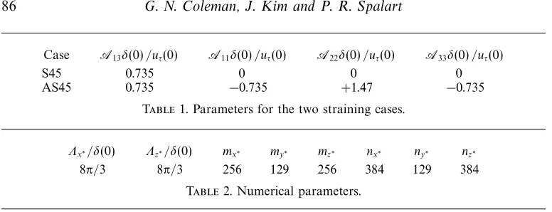
Case A13δ(0)/uτ(0) A11δ(0)/uτ(0) A22δ(0)/uτ(0) A33δ(0)/uτ(0)
S45 0.735 0 0 0
[image:12.595.104.492.114.263.2]AS45 0.735 −0.735 +1.47 −0.735
Table 1.Parameters for the two straining cases.
Λx∗/δ(0) Λz∗/δ(0) mx∗ my∗ mz∗ nx∗ ny∗ nz∗ 8π/3 8π/3 256 129 256 384 129 384
Table 2.Numerical parameters.
Solutions to (2.10) are obtained using a modified version of the spectral channel code of Kim et al. (1987). It expresses dependent variables as Fourier series in ξ1
andξ3, and via Chebychev polynomials in ξ2. No-slip conditions are enforced using the tau method (Lanczos 1956), and a mixed Crank–Nicolson/Runge–Kutta time-advance scheme is employed (Spalart, Moser & Rogers 1991). Further details of the solution procedure are given in the Appendix.
2.3. Cases
Two straining fields are considered here, defined by the components summarized in table 1. Both cases correspond to 3DBLs, in that the angle of sweep σ and there-fore the skewing A13 = A31 are non-zero. We choose σ = 45◦ and set A13 to
0.735 uτ(0)/δ(0) , the initial wall-friction-velocity to channel-half-width ratio. The rationale for these choices is given below. For now we note that the first case, denoted S45 (‘S’ to indicate non-zero skewing, ‘45’ the angle of sweep), has no normal compo-nents, and thus supplies the effect of a mean crossflow with no streamwise pressure gradient (PG); the second strain, Case AS45, combines skewing with streamwise deceleration and wall-normal stretching to create the deformation imposed by an idealized 45◦-swept wing (hence the notation AS45 – ‘A’ for adverse-pressure-gradient,
‘S45’ for σ= 45◦ skewing).
The numerical parameters used for both cases are listed in table 2, where Λx∗
and Λz∗ are the horizontal domain sizes in the principal-strain coordinates, and
(mx∗, my∗, mz∗) and (nx∗, ny∗, nz∗) are respectively the number of expansion coefficients
and collocation (quadrature) points in thex∗-,y∗-, andz∗-directions. Even though the
initial Reynolds number for these runs is the same as that used by Kim et al.(1987) for their two-dimensional study, Reτ=uτδ/ν ≈180, the three-dimensional nature of the present flows requires a larger computational expense (i.e. a square horizontal domain), due to the non-zero angle of sweep and the crossflow development. Aliasing (quadrature) errors are minimized by setting nx∗ = 3mx∗/2 and nz∗ = 3mz∗/2. (Total
aliasing-error control is not possible, since assigning n∗
y = 3m∗y/2 would compromise the no-slip boundary conditions.) Spectra and two-point correlations from Case AS45 atA13t= 0.125 are shown in figure 2, from locations near the wall and the centreline; Case S45 results are similar. The effect of the deformation, which for this case involves a compression in the x∗- direction, can be seen in the spectra by the shift of energy
to higher wavenumbers, compared to the initial distribution. In the correlations the influence of A∗
11 < 0 is apparent from the reduction of the length of maximum
streamwise separation (a measure of the largest structures that can be faithfully represented within the domain) from 0.5Λ∗
100
10–2
10–4
10–6
10–8
(a)
10–1 100 101 102 103
Spectra,
E
(
kx*
)
kx*d(0)
1.0
0.5
0
–0.5
(b)
0 0.1 0.2 0.3 0.4
Dx*/K
x*(0)
0.5
Cor
relations,
R
(
D
x
*)
100
10–2
10–4
10–6
10–8
(c)
10–1 100 101 102 103
Spectra,
E
(
kx*
)
kx*d(0)
1.0
0.5
0
–0.5
0 0.1 0.2 0.3 0.4
Dx*/K
x*(0)
0.5
Cor
relations,
R
(
D
x
*)
(d)
Figure 2.One-dimensional Fourier spectra and two-point correlations in principal-strain direction
x∗ for Case AS45: ——,u∗ component; - - - -, v∗; · · · ·, w∗. Curves with and without symbols respectively denoteA13t= 0.125 results and unstrained initial conditions at A13t= 0. (a, b) near centreline,yw/δ(0) = 0.805; (c, d) near walls,yw/δ(0) = 0.03.
correlations reveal that the resolution and domain size are sufficient to capture both the smallest and largest spatial structures.
Multiple Case S45 and AS45 simulations were performed using the same strain parameters for statistically independent realizations of the two-dimensional Poiseuille initial conditions. Theseσ= 45◦initial conditions were obtained by specifying that the
bulk flow rates in x∗ andz∗ be equal and running the strained-channel code with no
cU∞/cz
cW∞/cx
x
z
Outer-layer streamlines Fluid
element
X
X U∞ U∞
W∞
(a)
(b) x*
z* x
z
U∞
cU*
∞
cx*< 0
cW*
∞
cz* > 0
x = 0 x > 0
cU*
∞
cx*< 0
cW*
∞
cz* > 0
45°
45°
x*
z* x
z
Initial flow direction
r = 45°
* 11
* 33
x*
z*
* 11
* 33
(c)
Figure 3.Plan view of three-dimensional wall layer subjected to pure-skewing strain. (a) Spatially developing flow. Outer-layer streamlines and isobars very nearly coincide. (b) Strain applied to fluid element of spatially developing flow and strained-channel DNS. (Cross-hatched regions represent angular distribution of normal strains.) (c) Initial and deformed domain of strained-channel DNS for Case S45.
3. Results
3.1. Pure-skewing strain: Case S45
In order to determine the influence of pure three-dimensionality unaccompanied by the complications of streamwise pressure gradients, we set A∗
22 = 0, A∗11 = −A∗33 6= 0,
and choose an angle of sweep σ = 45◦. With respect to the initial flow direction,
the resulting strain field has only A13 = A31 as non-zero components, so that it
curved wind tunnel. Unlike the curved-duct flow, for which the streamwise gradient
∂P /∂x can only be zero at one spanwise location, here the strain field is the same at
every (x, z) point in the domain. (In the Schwarz & Bradshaw duct, along trajectories outside the centreline, the streamwise gradient through the bend is first adverse then favourable, and vice versa for paths closer to the centre of curvature; see their figure 2.) Another difference between the Schwarz & Bradshaw and present flows is in the magnitude of the skewing rate. The one used here, A13 = 0.735uτ(0)/δ(0) , is roughly twice as large, in terms of inflow uτ and boundary-layer thickness, as the
∂W /∂x imposed in the curved-duct experiment. For these reasons (and also because
of differences in Reynolds number, and downstream variation of the rate of skewing) we cannot expect the Schwarz & Bradshaw and Case S45 statistics to correspond. Nevertheless, the flows do share enough features that their comparative behaviour should be instructive.
3.1.1. Mean profiles and histories
The response of the mean velocity to the applied strain and in-plane wall motion (2.14) is illustrated in figure 4. These results validate the strained-channel methodology. A key characteristic of pressure-driven three-dimensional boundary layers can be seen, namely the sudden appearance of spanwise shear ∂ w/∂y(mean streamwise vorticity) in the outer layer, due to the A13-induced skewing of the mean spanwise vorticity.
The straining of the flow structures, away from their natural shapes in the two-dimensional flow, is also reproduced (although the same mean-flow behaviour could be obtained simply by injecting streamwise vorticity with a y-dependent body force, such an injection is unrealistic; the straining is required to correctly deform the outer-layer structures). The absence of streamwise acceleration (i.e. A11=A22 = 0) causes
the ‘thickness’ of the flow to remain constant, such that the distance δ between the wall and centreline in figure 4(a) is the same at all times (cf. figure 15 below). The inviscid skewing mechanism is thus the only mean-straining effect present in the outer layer. As a consequence, the ∂ w/∂y variation above the location of maximum w is inherited from the streamwise shear ∂ u/∂yof the initial flow. This explains the good agreement shown in figure 4(b) of the outer-layer hodograph with the straight solid lines, whose slopes are set by the Squire–Winter–Hawthorne (SWH) relationship, which assumes the mean velocity is governed solely by the effect of the skewing on the mean vorticity (Bradshaw 1987). For the present flow, using α to denote the angle through which the effective outer-layer mean velocity has turned due to the
A13 skewing, such that α = arctan(A13t), the SWH prediction gives u⊥ = uktan(2α),
where u⊥ and uk are respectively the velocity components orthogonal and parallel to
the current effective flow direction of the applied irrotational mean. The requirement that the mean velocity vector (u, w) change direction across a 3DWL is manifested by the finite curvature of the hodograph, as it describes the velocity distribution across both inner and outer layers. If inviscid skewing were to control the crossflow over the entire layer, and there were no near-wall shear-driven effects, the hodograph would be completely straight, and everywhere (including the origin) have the negative slope given by the SWH angle 2α. The result would be a collateral, rather than three-dimensional, flow.
1.0
0.5
0
0 0.5 1.0
(a)
yw d(0)
(w – ww)/uc(0) (u – uw)/uc(0)
(b)
0.2
0
0 0.2 0.4 0.6 0.8 1.0
u||/u||
c
u) u||
c
(c)
20
10
0
100 101 102
y+
Q+
Figure 4.Mean velocity evolution for Case S45: ——,A13t= 0 (α= 0◦); - - - -,A13t = 0.0625
(α= 3.6◦);· · · ·,A
13t= 0.125 (α= 7◦). (a) Axes aligned with initial mean flow. (b) Hodograph,
showing components (after wall velocities removed) parallel uk and normal u⊥ to instantaneous coordinates aligned with current direction of mean skewing (i.e. rotated away from principal-strain coordinates (x∗, z∗) by angle σ+α), normalized by parallel component at centreline uk
c; solid line segments denote SWH prediction. (c) Current wall-unit scaling; non-dimensional magnitude
Q+ ≡((u−u
w)2+ (w−uw)2)1/2/uτ(t) and wall-normal coordinate y+ = yw(0) exp (A22t)uτ(t)/ν, whereu2
τ(t) = ν[(∂u/∂y)2w+ (∂w/∂y)2w]1/2 is the current total wall-shear stress. Solid symbols are from two-dimensionalReτ= 180 channel of Kimet al.(1987).
the spanwise wall-shear stress has not propagated much higher than y+ ≈ 10 (cf.
figures 4aand 4c).
The histories of the centreline–wall velocity differences (∆uc,∆wc) responsible for the development of the inner layer are plotted in figure 5(a). The vertical lines in figure 5 indicate the times for which profiles are shown in other figures. These times, A13t = 0, 0.0625, and 0.125, respectively correspond to skewing angles of α = 0◦,
3.6◦, and 7◦. The streamwise ∆u
(a)
1.0
0.5
0 0.05 0.10 0.15
(D
uc,
D
wc
)/
uc
(0)
(b)
1.0
0.5
0 0.05 0.10 0.15
sw
(
t
)/
sw
(0)
kmax
(
t
)/
kmax
(0)
1.2
1.0
0.8
0 0.05 0.10 0.15
13t
(c)
Figure 5. Histories of (a) mean centreline–wall velocity difference (equation (3.1)), (b) surface shear stress and (c) maximum turbulence kinetic energy for Case S45: upper curves, streamwise components (∆uc =uc−uw in (a), (τw)x=ν(∂ u/∂y)w in (b)); lower curves, spanwise component (∆wc=wc−wwand (τw)z=ν(∂ w/∂y)w). Solid curve in (c) indicates maximum over allywlocations ofk=1
2u0iu0i; (cf. figure 6b) (note expanded vertical scale). Vertical lines mark times for which mean profiles are shown in other figures.
are respectively
uc(t) −uw(t)
uc(0) = cosh(−A13t), (3.1a)
wc(t) −ww(t)
uw)/uc(0) = 1.006 and 1.022 respectively at A13t= 0.0625 and 0.125. The spanwise-component history (3.1b) produces nearly linear growth of the effective crossflow at the centreline for the times considered (figures 4a and 5a), and ensures that the hodograph is correctly closed at the surface (figure 4b). This in turn develops the appropriate mean shear near the wall. Another measure of the rotational mean-flow development is shown in figure 5(b), where the upper curve traces the history of the streamwise mean skin friction, and the lower curve reveals the growth of the spanwise component, which is rapid. In contrast to ∆uc and ∆wc, which are functions only of A13t, the drag is affected by both the external forcing (applied strain) and the
turbulence. In the Schwarz & Bradshaw experiment the total skin-friction coefficient
Cf was observed to remain nearly constant through the bend, instead of increasing as in figure 5(b). However, since before entering the bend Cf was decaying with downstream distance, the levelling off in the curved section while the boundary-layer thickness kept increasing can perhaps be viewed as a milder form of the Cf increase seen here (furthermore, their perturbation was weaker).
The upward drift in time of the streamwise component of surface shear (figure 5b) might suggest that the turbulence near the wall has become more vigorous as the result of the applied skewing, but the histories of the turbulent stresses reveal the opposite. A stabilizing trend is apparent in figures 6(a) and 6(b) , which respectively show a reduction with time of the profiles of streamwise Reynolds shear stress −u0v0
and turbulence kinetic energy k = 1
2u0iu0i = 12q2. These reductions are more clearly
quantified in the sub-plots in the upper-right corners of figures 6(a) and 6(b), which illustrate the amount theA13t= 0.125 profiles have changed from their initial values (the figure 6ainset shows the net change to−u0v0; in figure 6(b) bothk(solid symbols)
and the vertical velocity variancev0v0(open symbols) are included). The decrease ofk
is also documented in figure 5(c), in terms of the history ofkmax, the largest value ofk
at each time. Figure 6(b) shows that askdecreases near the wall, the magnitude of the vertical velocity fluctuations v0v0 becomes larger across the entire layer. The issue of
the ultimate source of the near-wall reduction ofk and inner- and outer-layer growth of v0v0 will be addressed in the next subsection, where we consider the effect of the
skewing on the various terms in the Reynolds-stress budgets. We shall find there that budget terms involving the pressure fluctuations play a crucial role in the evolution of the turbulence. Foreshadowing this discovery is the amplification of the pressure fluctuations themselves, whose root-mean-square values are found in figure 6(c).† Of particular significance is the instantaneous pressure-fluctuation increase caused by the impulsive application of the strain (compare the thin and thick solid curves,
† There is a subtlety associated with diagnosing the pressure field associated with the diver-gence-free velocity in the strained-channel flow: because the grid deforms in time, spatial and temporal derivatives do not commute, which introduces an extra term in the Poisson equation. The kinematic pressurepsatisfiesp,ii=−u∗j,iu∗i,j−2u∗j,iA∗ij (note the factor 2).
Figure 6.Profiles of (a) shear stress, (b) turbulence kinetic energy, and (c) root-mean-square pres-sure fluctuations for Case S45: ——, A13t = 0 (α = 0◦); - - - -, A13t = 0.0625 (α = 3.6◦); · · · ·, A13t = 0.125 (α = 7◦) (data for A13t = 0.0625 not shown in (a) and (b) to
clar-ify presentation). Lower, middle, and upper curves in (a) respectively correspond to spanwise Reynolds shear stress −v0w0, streamwise Reynolds shear stress −u0v0, and total shear stress (τ)total = [(ν(∂ u/∂y)−u0v0)2+ (ν(∂ w/∂y)−v0w0)2]1/2. Subplots in (a) and (b) show change with
(a)
1.0
0.5
0
0 0.2 0.4 0.6 0.8 1.0
0.05
0
–0.05
0 0.2 0.4 0.6 0.8 1.0
s
/
sw
(0)
(b)
5
4
3
0 0.2 0.4 0.6 0.8 1.0
0
– 0.15
0 0.2 0.4 0.6 0.8 1.0
2
1
v
′
v
′/
u
2(0), s
k
/
u
2(0)s
(c)
0 0.2 0.4 0.6 0.8 1.0
2
1
(
p
′
p
′
)
1/2/
u
2(0)s
yw/d(0)
which respectively illustrate theA13t= 0 profiles just before and just after the strain is applied). Because of the elliptic nature of an incompressible flow, the pressure– velocity correlations in the Reynolds-stress budgets exhibit step changes in time, and thus dominate the early flow history of the stresses. This will be demonstrated in §3.1.2.
While the trend is for k and −u0v0 to both decrease, the −v0w0 shear stress does
the opposite, with the largest growth occurring nearyw/δ= 0.2 (figure 6a). However, although this component grows, it does so at a rate too small to immediately offset the reduction in −u0v0; the magnitude τ = (u0v02+v0w02)1/2 of the Reynolds-shear
stress ‘vector’ (−u0v0,−v0w0) also decreases in time. The decrease is very close to that
observed for the total (turbulent plus viscous) shear stress magnitude (τ)total (except
immediately adjacent to the wall), shown in the upper curves in figure 6(a). The extent to which these pure-skewing-induced changes are the result of deep structural alterations to the Reynolds-stress tensor is revealed in figure 7(a). This plot presents the stress/energy ratio τ/q2 (commonly given the symbol a1 and referred to as the
Reynolds-stress structure parameter), and shows it changes very little over most of the layer, with only a slight decrease of the maximum value. The implications of stress/energy-ratio reductions, a classical feature of perturbed 3DBLs, are twofold. From a fundamental point of view it implies that the extraction of kinetic energy from the mean by the turbulence has become less efficient. From a practical point of view it indicates an inaccuracy in turbulence models that assumea1 is constant for all
flows. The reduction seen in figure 7(a) is not large enough to pose a grave turbulence-modelling challenge; instead it demonstrates the degree to which the stress/energy ratio is (or rather is not) modified by a pure skewing strain. We shall see when we discuss Case AS45 that when the normal strain components are also non-zero the changes in a1 are much larger.
Another indication of the effect of the mean skewing upon the turbulence structure is given by the ratio of the turbulent flux of turbulence kinetic energy to the turbulence kinetic energy itself, v0(u0u0+v0v0+w0w0)/(u0u0+v0v0+w0w0). This ratio measures the
velocity Vq2 with which k = 12q2 is transported by the turbulence either toward (Vq2 <0) or away from (Vq2 > 0) the wall; it is plotted in figure 7(b). Unlike in the Schwarz & Bradshaw curved-duct experiment, where Vq2 was observed to decrease near the wall as the crossflow developed, and increase farther away, only minimal changes are produced by the Case S45 skewing. The source of this discrepancy is thought to be the off-centreline streamwise acceleration/deceleration, mentioned above, found in the duct flow (see also figure 18b below). The DNS results reveal that the impact of the pure skewing strain upon the turbulence structure is limited. Some aspects of modelling 3DWLs are therefore likely to be influenced less by mean three-dimensionality than by features unrelated to the introduction of mean crossflow. An attribute of the pure-skewing flow that will expose many turbulence models – any that assume isotropic eddy viscosity – is the lack of agreement between the direction of the mean shear and Reynolds shear stress. Differences as large as 30◦ are
observed, especially near the wall. This can be seen in figure 8. The sign change in the mean gradient angle γg = arctan [(∂ w/∂y)/(∂ u/∂y)] in figure 8(a) is a consequence of the sign change in ∂ w/∂y observed in figure 4(a). The modelling difficulty is in the finite time required for the spanwise shear to produce spanwise Reynolds stress −v0w0. The slow growth of−v0w0is another classical feature of non-stationary 3DBLs
(Schwarz & Bradshaw 1994). Because of it, the stress angleγ0
0.20
0.15
0.10
0.05
0 0.2 0.4 0.6 0.8 1.0
(a)
s
/
q
2
(b)
0.4
0.3
0.2
0.1
0
– 0.1
0 0.2 0.4 0.6 0.8 1.0
V2q
/
us
(0)
yw/d(0)
Figure 7. Profiles of (a) stress/energy ratio a1 = τ/q2 and (b) turbulent transport velocity
Vq2 =v0u0iu0i/q2 for Case S45: ——, A13t = 0 (α= 0◦); · · · ·, A13t = 0.125 (α= 7◦) (data for
A13t= 0.0625 not shown to clarify presentation). Reynolds-stress magnitudeτ= (u0v02+v0w02)1/2.
60
40
20
0
–20
– 40
0 0.2 0.4
60
40
20
0
–20
– 40
0 0.2 0.4
(a) (b)
cg
(de
g.)
cs
(de
g.)
yw/d(0) yw/d(0)
Figure 8.Direction of (a) mean shear γg and (b) Reynolds shear stress γτ for Case S45: ——, A13t = 0 (α = 0◦); - - - -, A13t = 0.0625 (α = 3.6◦); · · · ·, A13t = 0.125 (α = 7◦);
, A13t= 0.60 (single realization). Mean-shear angleγg = arctan[(∂w/∂y)/(∂u/∂y)]; Reynolds-stress angleγ0τ= arctan[−v0w0/−u0v0].
that γτ begins to follow (i.e. have the same sign but a smaller value than) γg in the outer region (compare the open symbols in figures 8(a) and 8(b), which show the variation of γg andγτ at A13t= 0.60). One of the primary goals of this project is to more fully understand the relationship between the mean shear (∂ u/∂y, ∂ w/∂y) and the (−u0v0,−v0w0) stresses, and to ascertain the implications for modelling suddenly
0.8
0.4
0
–0.4
0 0.2 0.4 0.6 0.8 1.0
0.05
0
– 0.05
0 0.2 0.4 0.6 0.8 1.0
Loss
Gain
yw/d(0)
Figure 9.Terms in the budget of turbulence kinetic energy k = 0.5u0
iu0i for Case S45: thin solid curves (——) denote terms atA13t= 0 (before strain); —·—,PS
k =12PiiS atA13t= 0.125;−−−−, −εk=−12εiiatA13t= 0.125; - - - -,Tk=12TiiatA13t= 0.125; —· ·—,Dk=12DiiatA13t= 0.125; · · · ·,Πk = 12Πii atA13t = 0.125;4,PkA = 12PiiA atA13t = 0.125; thick solid curve (---), sum of all terms (≈∂k/∂t) atA13t= 0.125 (also shown in inset with expanded vertical scale). Shaded regions indicate change from unstrained initial-condition profiles. Curves normalized by U4
ref/ν,
whereUref= 0.73uτ(0) .
0.8
0.4
0 0.2 0.4
yw/d(0)
PkS
Figure 10.Mean-shear productionPS
k =−u0v0∂ u/∂y−v0w0∂ w/∂yof turbulence kinetic energy for Case S45: ——,PS
k atA13t= 0;· · · ·,PkS atA13t= 0.125; —· ·—, product of−u0v0 atA13t= 0
and∂ u/∂yatA13t= 0.125. Normalization as in figure 9.
3.1.2. Reynolds-stress budgets
For the strained-channel flow, the non-dimensionalized transport equations for the Reynolds stresses reduce to
∂u0
iu0j
∂bt =Pij+Tij+Dij+Πij−εij, (3.2)
where the effective material derivative ∂/∂bt =∂/∂t+A22y∂/∂y (see §2), and right-hand-side terms are the rates of (cf. Mansour, Kim & Moin 1988)
production : Pij =−u0iv0 ∂ u∂yj −u0jv0 ∂ u∂yi −u0iu0`Aj`−u0ju0`Ai`,
dissipation :−εij =−Re2 ∂u
0
i
∂x`
∂u0
j