Variability of Stratospheric Ozone and Dynamics
Thesis by
Charles D. Camp
In Partial Fulfillment of the Requirements
for the Degree of
Doctor of Philosophy
California Institute of Technology
Pasadena, California
2004
c
° 2004 Charles D. Camp
Acknowledgements
I would like to thank the many people without whom this thesis would not have been
possible. Foremost is my advisor, Yuk Yung, whom I thank for his insightful guidance
and generous support. I am indebted to Michael Cross for his mentorship. I would
also like to thank Tapio Schneider and Andy Ingersoll for their advice and aid.
I would like to thank many graduate students, postdocs and staff for all the
en-joyable times and intriguing discussions. Chris Walker, Dave Noone, Xianglei Huang,
Shane Byrne, Sarah Stewart, Mark Roulston, Xun Jiang, Ron Henderson, Muruhan
Rathinam, Moira Regelson, Donal Gallagher, Russina Sgoureva, Chris Parkinson,
Mao-Chang Liang, Ben Lane, Claire Newman, Run-Lie Shia, thank you. I would
particularly like to thank David Hill, Beth Howard and Zhiming Kuang for all of the
many conversations and for their invaluable support.
I must thank Mike Black for all his help and Shawn Ewald and Ian McEwan for
all the discussions, technical and otherwise.
I am extremely grateful to two of my teachers, Sylvia Bonnell and Munzer Afifi,
for helping to put my feet on this path many years ago.
To my family, Anita, Ann, Nabil, Tarecq, Shirley, and Janet, thank you for all
you.
Abstract
This dissertation is a collection of empirical and modeling studies focusing on the
interannual variability (IAV) of stratospheric ozone and the dynamics associated
with that variability. Empirical analyses of the IAV of total column ozone in the
tropics and midlatitudes are performed using the Merged Ozone Data (MOD) set.
MOD combines the monthly mean column abundances collected by the Total Ozone
Mapping Spectrometer and the Solar Backscatter Ultraviolet instruments, provides a
nearly continuous record from late 1978 to present on a 2D grid. The first four EOFs
from principal component analyses of MOD capture over 93% (82%) of the variance
of the tropical (midlatitude) IAV. These analyses display structures attributable to
the quasi-biennial oscillation (QBO), with influence from a decadal oscillation, an
interaction between the QBO and an annual cycle (QBO-AB), and ENSO. Similar
decompositions occur for dynamical fields from the NCEP/NCAR reanalysis. Using
these analyses, we found possible connections between the deduced patterns in ozone
and the climate variables. For comparison to the observations, a 2D chemistry and
transport model (CTM) was used to simulate the ozone IAV. The NCEP/Department
of Energy (DOE) Reanalysis 2 data are used to derive a monthly mean meridional
allowing for an investigation of the impact of dynamics on the interannual variability
(IAV) of the total column ozone for all years for which the MOD is available. The 2D
CTM provides realistic simulations of the seasonal and IAV of ozone in the tropics,
reasonable agreement in the NH midlatitudes but poor agreement in the SH
midlati-tudes. The influence of the QBO and QBO-AB are well represented in the simulation.
A 71-year record of column ozone from Arosa, Switzerland is analyzed using singular
spectrum analysis (SSA). The SSA decomposition separates the signals from the
sea-sonal cycle, QBO, QBO-AB, and decadal oscillations. A 3.5-year oscillation is also
discovered. A nonlinear trend is extracted and nonstationary behavior of some of
the oscillations is found. Finally, a connection between fluctuations in stratospheric
Contents
Acknowledgements iii
Abstract v
1 Overview 1
2 Temporal and Spatial Patterns of the Interannual Variability of Total
Ozone in the Tropics 3
2.1 Introduction . . . 3
2.2 Datasets and Indices . . . 5
2.3 Methodology . . . 7
2.4 Ozone EOFs . . . 10
2.4.1 Merged Ozone Data (MOD) EOFs . . . 10
2.4.2 TOMS EOFs . . . 12
2.5 Analysis of the Ozone Decomposition . . . 14
2.5.1 QBO and Decadal . . . 14
2.5.2 Separating the QBO and Decadal Signals . . . 16
2.5.3 QBO-Annual Beat . . . 19
2.6 Analysis of NCEP/NCAR Data . . . 22
2.6.1 Layer Thickness EOFs . . . 23
2.6.2 100 hPa Surface EOFs . . . 25
2.7 Conclusions . . . 27
3 Interannual Variability of the Midlatitude Stratospheric Ozone: Ob-servations and Modeling 44 3.1 Introduction . . . 44
3.2 Analysis of the Merged Ozone Dataset . . . 49
3.2.1 Climatology . . . 49
3.2.2 PCA of MOD . . . 50
3.3 Simulating Ozone Transport in a 2D Chemical Transport Model . . . 54
3.3.1 NCEP-2 Derived Transport Fields . . . 54
3.3.1.1 Stream Function . . . 54
3.3.1.2 Isentropic Mixing Coefficient . . . 59
3.3.2 IAV of the Stream Function . . . 60
3.3.3 Simulated Total Column Ozone . . . 62
3.3.3.1 Climatology . . . 64
3.3.3.2 IAV . . . 66
3.4 Conclusions . . . 69
4.2 Singular Spectrum Analysis . . . 107
4.3 Analysis of Arosa Total Column Ozone . . . 110
4.3.1 Climatology and Spectral Analysis . . . 110
4.3.2 Decomposition Using Singular Spectrum Analysis . . . 111
4.4 Regression of SSA Components on NCEP Geopotential Heights . . . 113
4.5 Dependence on Window Length . . . 116
4.6 Nonstationary Behavior in the IAV of ATCO . . . 118
4.7 Discussion . . . 119
5 The Sensitivity of Tropospheric Methane to the Interannual Vari-ability in Stratospheric Ozone 149 5.1 Introduction . . . 149
5.2 Sensitivity to Interannual Fluctuations . . . 152
5.3 Simulating Interannual Fluctuations . . . 157
5.4 Discussion . . . 158
A Response of the Methane Evolution Equation to Various Forcings 167 A.1 Impulse Response . . . 168
A.2 Constant Forcing . . . 168
A.3 Single Period Oscillatory Forcing . . . 169
List of Figures
2.1 Standard deviations of the detrended, deseasonalized ozone time series
from the Merged Ozone Dataset. . . 32
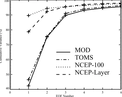
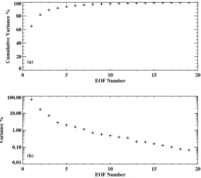
2.2 Cumulative variance as a function of number of EOFs. . . 33
2.3 Spatial patterns for the first four MOD EOFs. . . 34
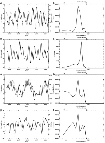
2.4 PC time series (left column) and spectra (right column) for the first
four MOD EOFs. PCs (solid lines) are shown along with an appropriate
index (dotted line). (a,b) PC1 and QBO index. (c,d) PC2 and inverted
Solar Flux. (e,f) PC3. (g,h) PC4 and SOI. . . 35
2.5 Spatial patterns for the fourth TOMS EOF. . . 36
2.6 PC time series (a) and spectrum (b) for the fourth TOMS EOF. PC4
(solid) is compared to the SOI (dotted). . . 36
2.7 Comparisons of filtered PCs of the MOD EOFs (solid) to appropriate
indices (dotted). (a) Bandpass A filtered PC1 and QBO index. (b)
Lowpass C filtered PC1 and Solar Flux. (c) Bandpass A filtered PC2
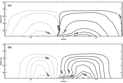
2.8 (a) Zonal averages of MOD EOF1 (solid line) and EOF2 (dashed line).
(b) Weighted sum (solid line) and difference (dashed) of the MOD EOF1
and EOF2 zonal averages. . . 37
2.9 Leading EOFs from the filtered MOD analyses. (a) EOF1 of the
Band-pass B filtered MOD (MOD-Band). (b) EOF1 of the LowBand-pass B filtered
MOD (MOD-Low). . . 38
2.10 PC time series (a) and spectrum (b) for the third EOF from the
Band-stop A filtered MOD data (MOD-Notch). . . 38
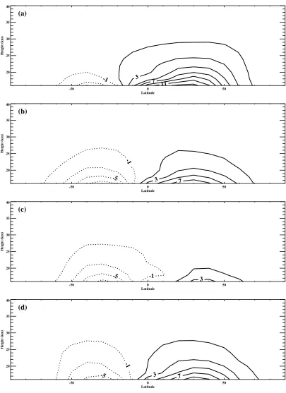
2.11 Spatial patterns for the first four EOFs from the NCEP/NCAR
reanal-ysis 30 hPa to 100 hPa layer thickness (NCEP-Layer). . . 39
2.12 PC time series (left column) and spectra (right column) for the first
four NCEP-Layer EOFs. PCs (solid lines) are shown along with an
appropriate index (dotted lines). (a,b) PC1 and Solar Flux. (c,d) PC2
and QBO index. (e,f) PC3 and SOI. (g,h) PC4. . . 40
2.13 Comparisons of filtered PCs of the NCEP-Layer EOFs to appropriate
indices. (a) Bandpass A filtered PC1 and QBO index. (b) Lowpass C
filtered PC1 and Solar Flux. (c) Bandpass A filtered PC2 and QBO
index. (d) Lowpass C filtered PC2 and inverted Solar Flux. . . 41
2.14 (a) Zonal averages of NCEP-Layer EOF1 (solid line) and EOF2 (dashed
line). (b) Weighted sum (solid line) and difference (dashed) of the
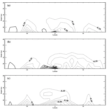
2.15 Spatial patterns for the first two EOFs from the NCEP/NCAR
reanal-ysis 100 hPa geopotential height data (NCEP-100). . . 42
2.16 PC time series (left column) and spectra (right column) for the first two
NCEP-100 EOFs. PCs (solid lines) are shown along with the appropriate
index (dotted line). (a,b) PC1 and Solar Flux. (c,d) PC2 and inverted
SOI. . . 42
2.17 Comparisons of filtered PCs of the NCEP-100 EOFs to appropriate
in-dices. (a) Bandpass A filtered PC1 and inverted SOI. (b) Lowpass C
filtered PC1 and Solar Flux. (c) Bandpass A filtered PC2 and inverted
SOI. (d) Lowpass C filtered PC2 and inverted Solar Flux. . . 43
3.1 Nov. 1978–Dec. 2002 mean of MOD. Units are DU. . . 72
3.2 Monthly means for MOD. Units are DU. (a) 1979–2002 Jan. mean. (b)
1979–2002 Mar. mean. (c) 1979–2002 May mean. (d) 1979–2002 Jul.
mean. (e) 1979–2002 Sep. mean. (f) 1979–2002 Nov. mean. . . 73
3.3 Nov. 1978–Dec. 2002 linear trend for MOD. Units are DU / decade. . 74
3.4 Standard deviation of the deseasonalized and detrended MOD. Units
are DU. . . 75
3.5 Relative and cumulative relative variance from the PCA of MOD. (a)
Cumulative relative variance. (b) Relative variance. . . 76
3.6 First 4 EOFs from PCA for MOD. (a) EOF1, (b) EOF2, (c) EOF3, (d)
3.7 First four PC time series and associated PSD from PCA for MOD. PC
time series (solid) shown with appropriate index (dotted). (a) PC1 and
QBO index. (b) PSD of PC1, (c) PC2, (d) PSD of PC2, (e) PC3 and
Solar Flux, (f) PSD of PC3, (g) PC4 and SOI, (h) PSD of PC4. . . . 78
3.8 (a) 1979–2002 mean of the isentropic mass stream function interpolated
to pressure surfaces. Units are 109kg/s. (b) 1979–2002 mean of the
isen-tropic velocity stream function interpolated to pressure surfaces. Units
are m2/s. . . . . 79
3.9 Mean seasonal cycle of the isentropic mass stream function. Units are
109kg/s. (a) 1979–2002 Jan. mean. (b) 1979–2002 Apr. mean. (c)
1979–2002 Jul. mean. (d) 1979–2002 Oct. mean. . . 80
3.10 Linear trends of the isentropic mass stream function. Units are 109kg/s/decade.
(a) Trend fit to entire dataset (all months). (b) Trend fit to Jan. only.
(c) Trend fit to Jul. only. . . 81
3.11 (a) 1979–2002 mean of the mean residual circulation stream function
scaled by density. Units are 109kg/s. (b) 1979–2002 mean of the mean
residual circulation stream function. Units are m2/s. . . . . 82
3.12 Isentropic mixing coefficient,Kyy, interpolated to pressure surfaces. Units
are 105m2/s. (a) Jan. 1985 (b) Apr. 1985 (c) Jul. 1985 (d) Oct. 1985 83
3.13 Relative and cumulative relative variance for PCA analysis of the
isen-tropic velocity stream function (a) Cumulative relative variance. (b)
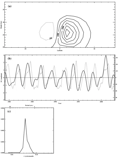
3.14 First EOF of the isentropic velocity stream function, associated PC time
series and its PSD. (a) EOF1; units are m2/s. (b) PC1 time series
(solid). Inverted QBO index (dotted). (c) PSD of PC1. . . 85
3.15 Second EOF of the isentropic velocity stream function, associated PC
time series and PSD. (a) EOF2; units are m2/s. (b) PC2 time series
(solid). Constructed QBO-AB index (dotted). (c) PSD of PC2. . . 86
3.16 Third EOF of the isentropic velocity stream function, associated PC
time series and PSD. (a) EOF3; units are m2/s. (b) PC3 time series
(solid). QBO index (dotted). (c) PSD of PC3. . . 87
3.17 1979–2002 mean column ozone abundances for 2D CTM simulated ozone
(solid) and zonally averaged MOD (dotted) . . . 88
3.18 1979–2002 mean column ozone abundances for individual months; 2D
CTM simulated ozone (solid) and zonally averaged MOD (dotted) (a)
1979–2002 Jan. mean. (b) 1979–2002 Apr. mean. (c) 1979–2002 Jul.
mean. (d) 1979–2002 Oct. mean. . . 89
3.19 Seasonal cycles in northern latitudes; 2D CTM simulated ozone (solid)
and zonally averaged MOD (dotted) (a) 55◦N, (b) 45◦N, (c) 35◦N, (d)
25◦N, (e) 15◦N, (f) 5◦N, . . . . 90
3.20 Seasonal cycles in southern latitudes; 2D CTM simulated ozone (solid)
and zonally averaged MOD (dotted) (a) 5◦S, (b) 15◦S, (c) 25◦S, (d)
3.21 Slope of the fitted linear trend for 1979–2002; 2D CTM simulated ozone
(solid) and zonally averaged MOD (dotted) . . . 92
3.22 Slope of the fitted linear trend for various months during the period
1979–2002. 2D CTM simulated ozone (solid) and zonally averaged MOD
(dotted) (a) 1979–2002 Jan. mean (b) 1979–2002 Apr. mean (c) 1979–
2002 Jul. mean (d) 1979–2002 Oct. mean . . . 93
3.23 Lowpass filtered, deseasonalized and detrended ozone anomalies for the
northern midlatitudes; 2D CTM simulated ozone (solid) and zonally
averaged MOD (dotted) (a) 55◦N, (b) 45◦N, (c) 35◦N. . . . 94
3.24 Lowpass filtered, deseasonalized and detrended ozone anomalies for the
northern subtropics and tropics; 2D CTM simulated ozone (solid) and
zonally averaged MOD (dotted) (a) 25◦N, (b) 15◦N, (c) 5◦N, . . . . . 95
3.25 Lowpass filtered, deseasonalized and detrended ozone anomalies for the
southern subtropics and tropics; 2D CTM simulated ozone (solid) and
zonally averaged MOD (dotted) (a) 5◦S, (b) 15◦S, (c) 25◦S, . . . . 96
3.26 Lowpass filtered, deseasonalized and detrended ozone anomalies for the
southern midlatitudes; 2D CTM simulated ozone (solid) and zonally
averaged MOD (dotted) (a) 35◦S, (b) 45◦S, (c) 55◦S, . . . . 97
3.27 Relative and cumulative relative variance for PCA analysis of the 2D
CTM simulated ozone. (a) Cumulative relative variance. (b) Relative
3.28 First EOF of the 2D CTM simulated ozone, associated PC time series
and PSD. (a) EOF1. (b) PC1 time series (solid). QBO index (dotted).
(c) PSD of PC1. . . 99
3.29 Second EOF of the 2D CTM simulated ozone, associated PC time series
and PSD. (a) EOF2. (b) PC2 time series. (c) PSD of PC2. . . 100
3.30 Third EOF of the 2D CTM simulated ozone, associated PC time series
and PSD. (a) EOF3. (b) PC3 time series (solid). QBO index (dotted).
(c) PSD of PC3. . . 101
3.31 Relative and cumulative relative variance for PCA analysis of zonally
averaged MOD. (a) Cumulative relative variance. (b) Relative variance. 102
3.32 First EOF of zonally averaged MOD, associated PC time series and
PSD. (a) EOF1. (b) PC1 time series (solid). QBO index (dotted). (c)
PSD of PC1. . . 103
3.33 Second EOF of zonally averaged MOD, associated PC time series and
PSD. (a) EOF2. (b) PC2 time series (solid). (c) PSD of PC2. . . 104
3.34 Third EOF of zonally averaged MOD, associated PC time series and
PSD. (a) EOF3. (b) PC3 time series (solid). (c) PSD of PC3. . . 105
4.1 (a)Arosa total column ozone (ATCO) withO(2) polynomial trend. (b)
Deseasonalized, detrended ATCO. (c) Mean seasonal cycle of ATCO.
(d) PSD of deseasonalized, detrended ATCO. Vertical (dotted) lines
4.2 (a) MEM spectra for ATCO of order 120 (solid), 140 (dotted), and
160 (dashed). Vertical (dotted) lines denote same periods as in Figure
4.1 (b)Adaptively weighted MTM spectrum for ATCO. Estimated
red-noise background and associated 90%, 95%, and 99% significance levels
are shown. The bandwidth parameter was set to p = 2 and K = 3
tapers were used. . . 123
4.3 Eigenvalue spectrum for the M270 SSA analysis of ATCO. . . 124
4.4 Leading pairs of EOFs for the M270 SSA analysis of ATCO; Solid
(dot-ted) line denotes first (second) member of each pair. (a) (1,2), (b)
(3,4), (c) (5,6), (d) (7,8), (e) (9,10), (f )(11,12), (g) (13,14), (h) (15)
unpaired. (i) (16,17), (j)(18,19). . . 125
4.5 Leading pairs of PCs for the M270 SSA analysis of ATCO, (a) (1,2),
(b) (3,4), (c) (5,6), (d) (7,8), (e) (9,10), (f ) (11,12), (g) (13,14), (h)
(15) unpaired. (i) (16,17), (j)(18,19). . . 128
4.6 Sum of the leading pairs of RCs for the M270 SSA analysis of ATCO,
(a) (1+2), (b) (3+4), (c) (5+6), (d) (7+8), (e) (9+10), (f ) (11+12),
(g) (13+14), (h) (15) unpaired. (i) (16+17), (j)(18+19). . . 131
4.7 PSDs of the RCs in the previous figure;(a)(1+2),(b)(3+4),(c)(5+6),
(d) (7+8), (e) (9+10), (f ) (11+12), (g) (13+14), (h) (15) unpaired,
4.8 (a) Partial reconstruction (solid) of ATCO time series (dotted) based
on first 20 EOFs of the M270 SSA analysis. (b) PSDs of the partial
reconstruction (solid) and raw ATCO (dotted). . . 136
4.9 (a) Regression coefficient for the regression of the M270 3.5-year
com-ponent (RCs 7+8) onto the NCEP 100 hPa geopotential height. (b)
t-statistic associated with the regression coefficient. . . 137
4.10 (a) Regression coefficient for the regression of the M270 3.5-year
com-ponent (RCs 7+8) onto the NCEP 30 hPa geopotential height. (b)
t-statistic associated with the regression coefficient. . . 138
4.11 (a) Regression coefficient for the regression of the M270 decadal
com-ponent (RCs 9+10) onto the NCEP 100 hPa geopotential height. (b)
t-statistic associated with the regression coefficient. . . 139
4.12 (a) Regression coefficient for the regression of the M270 QBO
compo-nent (RCs 11+12) onto the NCEP 30 hPa geopotential height. (b)
t-statistic associated with the regression coefficient. . . 140
4.13 (a) Regression coefficient for the regression of the M270 QBO-AB
com-ponent (RCs 13+14) onto the NCEP 30 hPa geopotential height. (b)
4.14 Comparison of various reconstructed IAV oscillations (solid curves), based
on pairs of M270 EOFs, to appropriate indices (dotted). (a) M270
3.5-year oscillation (RCs 7+8) and leading oscillation of a SSA analysis
of the PNA, (b) M270 decadal oscillation (RCs 9+10) and anomalous
sunspot number, (c) M270 QBO oscillation and the 30 hPa Singapore
wind, (d) M270 QBO-AB oscillation and a QBO-AB index. . . 142
4.15 Eigenvalue spectra for M155 and M85 SSA analyses of ATCO. (a) M155
(b) M85. . . 143
4.16 Comparison of the 3.5-year oscillations found in SSA analyses of ATCO
for various window lengths. (a) sum of paired RCs (7,8) from the M155
(solid) and M270 (dotted) analyses. (b) sum of paired RCs (5,6) from
the M85 analysis. . . 144
4.17 Comparison of the trends found in SSA analyses of ATCO for various
window lengths plotted against the original ATCO (black line): M =
270 (red), 155 (green), and 85 (blue). . . 145
4.18 Comparison of the annual cycle found in SSA analyses of ATCO for
various window lengths (a) M = 270,(b) M = 85, (c)M = 12. . . . 146
4.19 Power spectral estimates of 30 year segments of the deseasonalized,
de-trended ATCO. Segments begin every 5 years staring in 1933. Vertical
dotted lines mark periods of 11 years, 3.5 years, 28 months and 20
5.1 (a) Fractional change in ozone column abundance from the merged
SBUV/TOMS dataset. (b) Spectrum of the ozone data. The solid
line is the filtered data or spectrum and the dotted line is the unfiltered
data or spectrum. . . 162
5.2 (a) Fractional change in methane abundance from the NOAA-CMDL
flask monthly means database. (b)Spectrum of the methane data. The
solid line is the filtered data or spectrum and the dotted line is the
unfiltered data or spectrum. . . 163
5.3 Estimates of the delay of the methane response to the ozone forcing.
(a) Cross correlation of the changes in ozone and methane abundances
for the 1984–1998 period. The delay can be estimated by the lag
cor-responding to the maximum cross correlation. (b) Plot of G(L) from
Equation (A.16). The delay can be estimated by the lag corresponding
to the first positive root. . . 164
5.4 Paired ozone-methane changes (with a 6 month delay). The sensitivity,
αCH4, is the slope of the least squares linear fit (solid line) to the paired
data. Data between Apr. 1984 and Dec. 1991 are denoted by +’s. Data
between Jan. 1992 and Dec. 1998 are denoted by ¦’s. Least square
linear fits are shown for the data prior to 1992 (dotted line) and the
5.5 (a)Comparison of the filtered methane data (solid line) to filtered ozone
data (dotted line). The ozone data has been shifted up 6 months and its
amplitude has been multiplied by the sensitivity,αCH4. (b)Comparison
of the filtered methane data to the simulated methane response (dotted
List of Tables
2.1 Frequency Filters . . . 30
2.2 Correlations between TOMS and MOD PCs and Various Indices . . . . 30
2.3 Correlations between NCEP/NCAR Reanalysis PCs and Various Indices 31
3.1 Correlations between MOD PCs and Various Indices . . . 71
3.2 Correlations (Lag = 0) and Maximum Cross Correlations of the Stream
Function PCs with Various Indices. The numbers in parentheses denote
significance levels. Units of lag are month. Positive (negative) lags
correspond to the PC time series leading (trailing) the indices. . . 71
3.3 Correlations between 2D Model Ozone and Zonal MOD. . . 72
4.1 Clustered eigenvalues and the periods of the associated oscillations for
three SSA analyses. Clusters which satisfy a same-frequency test are
5.1 Calculated sensitivity, αCH4, of the methane response to ozone
fluctuations. The sensitivity is estimated by the slope of the linear fit
to the paired ozone and methane data, as shown in Figure 5.4. Values
are shown for the entire time domain and for a partition of the time
domain. Values for the intercepts of the linear fits are also given. . . . 161
5.2 Correlations between the methane observations, (CH4)d, and
the ozone observations, O3, and the simulated methane
re-sponse,(CH4)s.The coefficient of determination (R2), associated Fisher
Z significance and estimated degrees of freedom are also shown. . . 161
5.3 Sensitivity, αX, of tropospheric chemical species X to
strato-spheric ozone changes for the period 1979–1994. The values
reported here correspond to the relative change in global tropospheric
annual average levels in X (%) resulting from a 1% decrease in total
column ozone; the assumed scenarios are discussed in the cited
publi-cations. The type of model used is indicated in parentheses. Note that
the values of Granier et al. (1996) correspond to the 1990–1994 period.
The calculations indicated as Granier-1997 correspond to the 1979–1994
period and have been obtained using an updated version of the model
Chapter 1
Overview
This dissertation is a collection of empirical and odeling studies focusing on the
in-terannual variability (IAV) of stratospheric ozone and the dynamics associated with
that variability.
Chapter 21 studies the IAV of the tropical total ozone column as seen in satellite
observations. A principal component analysis is used to determine the dominant
pat-terns of variability. Results are then compared to dynamical fields from the National
Centers for Environmental Prediction (NCEP)/ National Center for Atmospheric
Research (NCAR) reanalysis in order to connect physical processes to the observed
modes of variability.
Chapter 32 extends the tropical analysis into the midlatitudes. In addition,
ozone IAV is simulated using a two-dimensional chemical transport model driven
by a monthly mean meridional circulation derived from the NCEP/NCAR
reanaly-1Chapter 2 has appeared as “Temporal and spatial patterns of the interannual variability of
total ozone in the tropics” inJ. Geophy. Res.,108(D20)(2003), 4643, doi:10.1029/2001JD001504
(co-authored with Mark S. Roulston and Yuk L. Yung). It is reproduced in this dissertation with permission of the publisher.
2Portions of Chapter 3 are to appear as “QBO and QBO-annual beat in the tropical total column
ozone: A two-dimensional model simulation” inJ. Geophy. Res., (2004), doi:10.129/2003JD004377
sis. Simulated ozone results are compared to satellite observations of ozone. I would
like to acknowledge Xun Jiang and Run-Lie Shia for their work in deriving the stream
function and running the 2D model.
Chapter 4 is a singular spectrum analysis (SSA) of a 71-year record of column
ozone from Arosa, Switzerland. This long continuous record allows a detailed study
of the IAV to be performed and the SSA technique allows intermittent, anharmonic
oscillations and nonlinear trends to be extracted.
Chapter 53 is an investigation of a mechanism by which IAV variability in
strato-spheric ozone affects concentrations of tropostrato-spheric methane. This is an unusual mode
of stratospheric-tropospheric interaction, in which UV radiation to couple
strato-spheric dynamics to tropostrato-spheric chemistry.
3Chapter 5 and Appendix A appeared as “The sensitivity of troposheric methane to the
interan-nual variability in stratopsheric ozone” inChemosphere — Global Change Science,3(2001), 147-156
Chapter 2
Temporal and Spatial Patterns of
the Interannual Variability of Total
Ozone in the Tropics
2.1
Introduction
The total column abundance of ozone in the atmosphere represents an intricate
inter-action between chemical and dynamical processes (see, for example, Brasseur et al.
(1999)). A primary motivation for studying the interannual variability (IAV) of
to-tal ozone is to separate anthropogenic perturbations of the ozone layer from natural
variability (see, for example, WMO (1999)). The latter imposes “noise” on the
sys-tem that makes the detection of ozone depletion and its attribution to anthropogenic
forcing more difficult. In addition, the IAV offers insights into the subtle coupling
between chemistry and dynamics that are important for determining the abundance
and distribution of ozone, as well as providing opportunities to test the sensitivity of
models to external and internal forcing.
An extensive global dataset is currently available for studying IAV of ozone. The
space-craft measured the spatial distribution of total ozone from 1978 until 1993 (Herman
et al., 1991). By scanning across the track of the satellite, TOMS obtained data
be-tween successive satellite orbital tracks. Daily TOMS gridded ozone data of Version
7 (McPeters et al., 1996) (on a 1◦×1.25◦ grid in latitude and longitude) are available
from 1979 to 1992. The data were extended to 2000 (on a 5◦×10◦ grid) in the the
Merged Ozone Datasets (MOD), which combine the monthly mean column
abun-dances of the of TOMS instruments on Nimbus 7 and Earth Probe with additional
data from the Solar Backscatter Ultraviolet (SBUV and SBUV/2) instruments on
Nimbus 7, NOAA 9, NOAA 11 and NOAA 14.
Previous studies have fruitfully mined the rich TOMS dataset. Using globally
averaged TOMS data,Herman et al.(1991) detected the ozone depletion trend,
quasi-biennial oscillation (QBO) and a possible 11-year solar cycle variation. Using zonally
averaged TOMS data, Tung and Yang (1994a,b) studied the propagation of QBO
effects from the tropics to the midlatitudes, and the interaction between the QBO
and the annual cycle, giving rise to 20-month and 8.6-month oscillations. Shiotani
(1992) studied the zonal variability of ozone in the tropics related to the El Ni˜
no-Southern Oscillation (ENSO) andKayano (1997) carried out an empirical orthogonal
function (EOF) study of the relation between total ozone and ENSO.
However, we notice the curious omission of a simultaneous decomposition of the
TOMS data to reveal all spatial and temporal patterns in the tropics. This paper
attempts to fill this gap in our analysis of total ozone.
more variability than the tropics. This can be seen in Figure 2.1, which shows the
standard deviations for the time series at each grid point of the detrended,
deseason-alized Merged Ozone Data. (Details of this dataset and its processing are described
in the following section.) The inclusion of data from higher latitudes in the
analy-sis would result in EOF patterns dominated by midlatitude signals. Therefore, the
tropical patterns would be much harder to isolate and analyze.
In Section 2.2, the datasets and indices used are described. In Section 2.3, the
EOF technique is briefly discussed. The results of the EOF analysis of the ozone
data are shown in Section 2.4. Comparisons of this analysis to physical processes are
discussed in Section 2.5. In Section 2.6, an EOF analysis of the NCEP/NCAR data
is shown and compared to the ozone results. Section 2.7 contains conclusions and
final remarks.
2.2
Datasets and Indices
For this study, we have used two datasets for monthly mean column ozone abundances:
Nimbus 7 TOMS (McPeters et al., 1996) and the Merged Ozone Data (MOD) as
described in the NASA website,
http://code916.gsfc.nasa.gov/Data services/merged/mod data.public.html.
For both datasets, we have restricted our analysis to a tropical band from 25◦S to
25◦N. To lower the computational load of the EOF analysis, the TOMS data has been
rebinned from its original 1◦×1.25◦ grid to a 2◦×7.5◦ grid. The MOD data is on a
MOD data from Nov. 1978 to Dec. 2000.
Data from the National Centers for Environmental Prediction and National
Cen-ter for Atmospheric Research (NCEP/NCAR) reanalysis were also analyzed (Kalnay
et al., 1996). To match the analyses performed on the ozone datasets, we restricted
the EOF analysis of the NCEP/NCAR fields to the 25◦S to 25◦N tropical band. The
data were also rebinned from the original 2.5◦×2.5◦ grid to a 2◦×7.5◦ grid. Cubic
spline interpolation was used to refine the latitude spacing. The EOF analysis was
performed on data from Jan. 1979 to Sept. 1999.
All datasets were detrended by removing the linear long-term trends from the
time series of each grid point; the linear trends were determined by a least squares
fit. Seasonal cycles for each time series were also removed; cycles were determined by
taking averages for each month independently. Missing months were replaced by cubic
spline interpolation in time. To isolate interannual variability from higher-frequency
oscillations, further filtering was performed spectrally. The spectral filter applied was
a convolution of a step function with a Hanning window chosen to obtain a full signal
from periods above 15 months and no signal from periods below 12.5 months; see
Press et al.(1992, Chap.13). The details of this filter, Lowpass A, and other similarly
constructed filters used in this study are shown in Table 2.1.
Various indices were used to help identify the processes seen in the EOF analyses.
For a QBO index, we used the QBO Zonal Wind Index, 1953–September 2001. For
our time interval, this index uses the 30 hPa zonal wind measured above Singapore
Marquardt and Naujokat (1997). For an ENSO index, we used the SOI:
Standard-ized Sea Level Pressure Anomaly time series described in the International Research
Institute for Climate Prediction (IRI) web site:
http://ingrid.ldgo.columbia.edu/SOURCES/.Indices/.soi/ .dataset documentation.html.
For a solar cycle index, we used the Adjusted Monthly Solar Flux: 2800 MHz Series
C time series, described on the NOAA web site:
http://spidr.ngdc.noaa.gov/spidr/help/solar main.htm#flux.
Linear detrending and lowpass filtering, using the Lowpass A filter, were performed
on all indices.
For presentation purposes only, the data for all color figures have been bilinearly
interpolated to a much finer spatial resolution.
2.3
Methodology
Given a multivariate dataset consisting of measurements from S stations taken
si-multaneously atT times, the EOFs are found by determining the eigenvectors of the
covariance matrix, C, of the dataset constructed from the T measurement vectors,
xt (i.e. the state of the system at time t) (Preisendorfer, 1988). If X is the matrix
given by X = [Xt]∗ (T ×S) and the temporal means of the data from each station
have been removed, then the covariance matrix is given by
C= 1
TX
∗X (S
The covariance matrix is a real symmetric positive-semidefinite matrix and can
there-fore be written as
C=QΛQ∗ (2.2)
whereΛis a diagonal matrix whose elements are the S real, nonnegative eigenvalues,
λ, and Q is a orthogonal matrix whose columns are theS orthonormal eigenvectors,
e. These eigenvectors are the EOFs and form a new basis with which the original
data can be represented,
X=PQ∗ =Xpe∗ (T ×S) (2.3)
P is a (T ×S) matrix whose columns, p, are the S principal component time series
(PCs) determined by projecting the original dataset onto the associated EOFs,
p =Xe (2.4)
Combining equations (2.1),(2.2) and (2.3), we can see that
Λ= 1
TP
∗P (2.5)
SinceΛ is diagonal, the PCs (p) are mutually orthogonal and the eigenvalues (λ) are
equal to their variances. In the context of this study, the EOFs can be considered
two-dimensional spatial standing waves while the associated PCs are the time-dependent
cap-tured by each EOF. When sorted by decreasingλ, the leading neigenvectors (EOFs)
describe more variance than any other n vectors.
It is clear from Equation 2.3 that an arbitrary scaling factor can be applied to
the EOFs, if it is simultaneously removed from the associated PC. One convention
is to normalize the EOFs, kek = 1; then the variance of the associated PCs will be
equal to the associated eigenvalues. However, to present our results more clearly, we
wanted the EOF patterns to have dimensional units. Therefore we have multiplied
the EOFs (and divided the PCs) by the square root of their associated eigenvalue,
i.e., the standard deviation of the conventional PC. Therefore our PCs have been
normalized to have unity standard deviation, while the EOFs display typical values
of the amplitude of oscillation at each grid point. The peak-to-trough amplitudes of
the oscillations at any grid point can be recovered by taking the product of the EOF
value and the peak-to-trough amplitude of the associated PC time series.
Significance statistics for correlations between time series, such as PCs and
in-dices, were generated by a Monte Carlo (bootstrap) method (Press et al., 1992, chap.
15). Three thousand isospectral surrogate time series (same power spectrum,
ran-domized phases) were generated for each comparison to create a distribution of
corre-lations. This distribution was transformed into an approximately normal distribution
by the Fisher transformation (Devore, 1982). The significance level of the actual
(transformed) correlation within the transformed-correlation distribution was then
2.4
Ozone EOFs
EOF analyses were performed on the [25◦S, 25◦N] latitude band of the detrended,
deseasonalized MOD and TOMS datasets. The patterns found in the decomposition
of MOD are quite robust; analyses performed on other latitude bands have very
similar patterns and symmetries. The TOMS analysis has the same features as the
MOD analysis; however, they appear in different combinations within the first few
EOFs than they do in the MOD analysis. The relationship between the derived
spatial patterns, their associated time series and physical processes will be discussed
in Section 2.5.
2.4.1
Merged Ozone Data (MOD) EOFs
The first four EOFs of MOD together account for more than 93% of the variance, as
shown by the solid line in Figure 2.2. The spatial patterns associated with these EOFs
are shown in Figure 2.3. The associated PC time series and their Fourier spectra are
shown in Figure 2.4. Each PC is shown in comparison to an appropriate index.
The first EOF (MOD EOF1) captures 42% of the variance of MOD. It is basically
a meridional arc showing zonal uniformity and symmetry about the equator. It
oscillates about nodes at latitudes approximately 15◦ off the equator. The values
shown range from a high of 7.0 Dobson units (DU) on the equator to a low of −2.8
DU at the northern boundary. The associated PC time series (MOD PC1), given in
Figure 2.4a, shows the amplitude of the oscillation of this EOF in MOD. A maximum
The spectrum of the PC, Figure 2.4b, shows a dominant peak at 28 months with a
secondary decadal signal. There are additional peaks at approximately 18 months and
4 years. Figure 2.4a shows the PC (solid line) compared to the QBO index (dotted
line).
A quick comment about the fine-scale features of the EOFs: While the maximum
of MOD EOF1 actually appears to occur a couple of degrees south of the equator, we
are reluctant to subscribe any significance to this asymmetry (as well as to other
fine-scale behavior in this and following EOF patterns). Since MOD has 5◦ latitude bins,
we can only say that the maximum occurs between 2.5◦N and 2.5◦S. Furthermore, the
fine-scale features are not robust between analyses, whereas the qualitative nature is.
The second EOF (MOD EOF2) is similar to MOD EOF1 in that it is basically
a zonally uniform and equatorially symmetric meridional arc, albeit with somewhat
more zonal structure than MOD EOF1. It captures 33% of the variance of MOD.
However, the pattern is almost entirely negative, barely breaking zero only at the
equator. The maximum of 0.9 DU lies on the equator and the minimum of −6.4 DU
at the northern boundary. It is thus very similar to EOF1 except for a DC shift (i.e.,
a spatially constant offset). The associated PC (MOD PC2)is shown in Figure 2.4c.
The spectrum of the PC, Figure 2.4d, has the same two primary peaks, 28 months
and decadal, but the decadal is clearly dominant.
The third EOF (MOD EOF3), capturing 15% of the variance, is a tilted plane
oscillating about the equator. The pattern is still roughly zonally uniform, but it is
−4.1 DU in the south. The spectrum of the associated PC, shown in Figure 2.4f, has a single dominant peak at 21 months.
The fourth EOF (MOD EOF4), capturing less than 4% of the variance, is the
first occurrence of a pattern with strong zonal structure. Roughly symmetric about
the equator, the EOF is a standing wave oscillating about nodes in the western and
eastern Pacific. Values range from 2.1 DU in the central Pacific to −3.1 DU over
Indonesia. The spectrum of the associated PC, Figure 2.4h, is fairly broad with its
highest peak at a period of 4 years and substantial power in periods greater than 5
years.
Analyses performed on MOD for [20◦S, 20◦N] and [30◦S, 30◦N] latitude bands
(not shown) display very similar results to the analysis of [25◦S, 25◦N] band of MOD
described above.
2.4.2
TOMS EOFs
The EOF decomposition of the TOMS dataset displays the same features as described
above for the MOD analysis, albeit in a different combination. The TOMS dataset has
a finer spatial resolution than MOD, but a shorter time series. Therefore the EOFs
show more detail, but the PCs are in general noisier and the spectra less resolved. In
particular, with only 14 years of data, all correlations with decadal signals must be
treated with great caution.
The first four EOFs capture over 94% of the variance of TOMS with basically
first three TOMS EOFs and PCs (not shown) contain the same basic structures as
the equivalent MOD EOFs and PCs, but in a different combination than that seen
in the MOD analysis. TOMS EOF1 shows the meridional arc and its associated
spectrum shows the 28-month peak. TOMS EOF2 shows a combination of a tilted
plane and a DC shift with its spectrum dominated by a broad low-frequency band
(7–10+ years) and a secondary peak at 20 months. TOMS EOF3 shows a tilted
plane (its node slightly offset from the equator) and a dominant 20-month peak with
a secondary low-frequency signal. These are the same features that appear in the first
three MOD EOFs and PCs, but they have been shuffled somewhat. In the TOMS
decomposition, the DC shift and decadal components are combined with the tilted
plane and 20-month signals in the second and third EOFs/PCs, as opposed to being
combined with the meridional arc and 28-month signals as occurs in the first and
second EOFs/PCs of the MOD analysis. This conflation of signals is discussed in
detail in Section 2.5.2.
Like MOD EOF4, the fourth TOMS EOF (Figure 2.5) is the first appearance of a
pattern with a primarily longitudinal oscillation; however, it has a somewhat different
structure. Both EOFs show rough equatorial symmetry and a zonal oscillation with
nodes in the central and western Pacific. But in TOMS EOF4, there is a
double-ridged symmetric structure with ridges at 12◦N,S and maxima thereof at 150◦W;
this structure was not present at the lower spatial resolution of MOD EOF4, which
exhibited a maximum near the equator at 150◦W. Furthermore, TOMS PC4, Figure
2.4h, despite coming from a shorter dataset.
2.5
Analysis of the Ozone Decomposition
The patterns seen in both the MOD and TOMS EOF decompositions can be closely
tied to dynamical processes in the atmosphere. Most of the structure in the first four
EOFs of both datasets can be attributed to three physical processes: the QBO, the
interaction between the QBO and annual cycles, and ENSO. There is also substantial
contribution from a process (or multiple processes) fluctuating on decadal time scales.
With the exception of the decadal behavior and (to a much lesser degree) ENSO, the
EOF analyses separate these processes into distinct EOFs. The correlations between
indices for the physical processes and the PCs of both MOD and TOMS are listed in
Table 2.2.
2.5.1
QBO and Decadal
Ignoring for the moment the decadal signal, the dominant pattern seen in the first
two EOFs of both datasets is the meridional arc structure oscillating with a period
of 28 months. These are the spatial and temporal characteristics of the effect of
the QBO on the ozone. Ozone is primarily created in the tropics of the middle
stratosphere and carried poleward by the Brewer-Dobson circulation. This zonal
mean meridional circulation is slow compared to the mean zonal wind. Therefore the
spatial patterns of tracer transport associated with it should be zonally uniform to
Brewer-Dobson circulation (Plumb and Bell, 1982; Baldwin et al., 2001). Therefore
the tropical column ozone will increase (decrease) while the opposite will occur at
higher latitudes. The phase change of this effect occurs at approximately 12◦ north
and south of the equator (Tung and Yang, 1994a). The patterns of both EOFs are
roughly characteristic of the QBO, but the nodes of the EOFs appear to occur at
the wrong latitudes. Furthermore, the appearance of two very similar EOFs and the
conflation of the QBO and decadal signals obscures the connection to either process.
These points will be revisited later in Section 2.5.2.
The source of the decadal signal is an area of active research. One strong candidate
is the decadal variation in the solar flux (Chandra and McPeters, 1994; Shindell
et al., 1999). An increase in insolation leads to an increase in net ozone production.
However, it has been demonstrated that this cannot account for all of the amplitude
of the decadal variation (WMO, 1999). Furthermore, the solar cycle appears to
have a more complicated relationship with some of the other processes involved. For
example, the length of the positive and negative phases of the QBO may be affected
by the solar cycle (Salby and Callaghan, 2000).
For better comparison to the QBO and Solar Flux indices, MOD PC1 and PC2
were filtered to isolate the two signals. The Bandpass A filter (Table 2.1) was used to
remove the decadal contribution. The filtered PCs are compared to the QBO index
in Figures 2.7a,c. The Lowpass C filter was used to remove the QBO contribution.
Figures 2.7b,d show the results in comparison to the Solar Flux index. These indicate
MOD PC2 has a positive correlation with the QBO but a negative correlation with
the Solar Flux.
2.5.2
Separating the QBO and Decadal Signals
The conflation of decadal and QBO signals in the first two EOFs and the appearance
of similar patterns in the two orthogonal EOFs need further examination. It is unclear
from the original EOF analysis whether the decadal signal is independent of the QBO
time scale signal or if it is a low-frequency variation in the higher-frequency signal.
Since both EOFs are roughly zonally uniform, it is simpler to explore the zonal
averages of the EOFs, shown in Figure 2.8a. MOD EOF2 (dashed line) is basically a
constant shift of MOD EOF1. Recalling the filtered PCs, Figures 2.7a–d, both MOD
EOF1 and EOF2 are positively correlated with the QBO index. Therefore, on QBO
time scales, EOF1 and EOF2 oscillate in phase. But EOF2 is inversely correlated to
the Solar Flux, while EOF1 is positively correlated, so on decadal time scales they
oscillate a half period out of phase. Therefore the QBO contribution is the weighted
sum of the two EOFs, while the decadal contribution is the weighted difference.
The weights for the sum can be determined by finding the standard deviation of
the Bandpass A filtered PCs. They roughly represent the portion of the amplitude
of the oscillation of each EOF attributable to QBO time scales. The weights for
the difference can be determined by finding the standard deviation of the Lowpass
C filtered PCs and represent the portion attributable to decadal time scales. The
in the manner are shown in Figure 2.8b. This suggests that, for the combination
of the first two EOFs, the QBO time scale signal is a meridional arc with nodes at
approximately 11◦ off the equator, while the decadal signal is roughly a flat plane
with no nodes. Thus, by separating the QBO and the decadal contributions, we have
recovered the expected structure for the QBO signal and identified one for the decadal
variability.
The same procedure can be performed with the full EOFs instead of the zonal
averages and an associated time series can be found by projecting the original data
onto these constructed patterns. However, these patterns and time series will no
longer be mutually orthogonal.
A more rigorous way to separate the decadal and QBO time scale signals is to filter
the data for the desired frequencies prior to performing the EOF analysis. It should
however be noted that disadvantages of this method include the loss of the ability
to examine long-term fluctuations of shorter time scale features and the possible
distortion of highly nonsinusoidal signals when narrow-bandwidth Fourier filtering is
applied. These caveats notwithstanding, this procedure is a useful confirmation of
the previous linear combination method. This procedure was performed using the
Bandpass B and Lowpass B filters described in Table 2.1. The leading EOFs of the
resulting analyses are shown in Figure 2.3. These EOFs are very similar to those
found by the linear recombinations of the full (2D) MOD EOF1 and EOF2 (data not
shown).
81% of the variance of the filtered dataset, display patterns associated with the QBO
without the interference from any decadal process(es). Obvious signs of ENSO are
also removed, although higher harmonics of ENSO’s fundamental period may still be
present. These harmonics are discussed later in more depth.
The first EOF, Figure 2.9a, captures 61% of the variance. It shows the QBO
pattern with nodes at approximately 12◦ off the equator. Values range from 6.3 DU
at the equator to −4.8 DU at the northern boundary. The associated PC (data not
shown) correlates well with the QBO index; see Table 2.2. Its spectrum is very similar
to the portion of the MOD PC1 spectrum contained between periods of 1 to 3 years;
see Figure 2.4b. The second EOF (data not shown) captures 20% of the variance. It
shows a tilted plane pattern similar to that of MOD EOF3, Figure 2.3c. This pattern
is characteristic of the QBO-annual beat, described later in this section. Values are
similar, ranging from 3.6 DU in the north to −2.8 DU in the south, and there a little
more longitudinal structure. The spectrum of the associated PC shows a clean peak
at 21 months, again similar to MOD PC3, Figure 2.4f.
The first EOF of the Lowpass B filtered MOD (MOD-Low), Figure 2.9b, captures
over 76% of the variance of the filtered data. It is roughly a flat plane with no nodes;
values are strictly positive, ranging from 4.0 DU to 2.0 DU. This DC component seems
to be a consistent feature of the patterns associated with decadal variability. The
associated PC correlates well with the Solar Flux index; see Table 2.2. Its spectrum
shows a strong decadal peak and a weaker broad peak at 3.5–4.5 year periods. This is
of this EOF. The decadal signal can be separated from the ENSO signal by a tighter
filter,e.g. the Lowpass C filter. However, this restrictive a filter would leave very few
degrees of freedom in the resulting time series, so the resulting EOF analysis might
not be very robust.
2.5.3
QBO-Annual Beat
The third MOD EOF displays a tilted plane oscillating about a node at the equator
with a period of 21 months. These are spatial and temporal characteristics of the
interaction between the QBO and annual cycles. The modulation of the annual
merid-ional transport by the tropical QBO results in the creation of two beat oscillations
with frequencies equal to the sum and difference of the QBO and annual frequencies,
i.e., at periods of 21 and 8.4 months (Tung and Yang, 1994a; Baldwin et al., 2001).
While this process is primarily an extratropical one, its effects can be seen inside
the [25◦S, 25◦N] band of this study. However, the interaction between the QBO and
any annual cycle (e.g. the annual cycle in ozone production) has the potential to
create identical beat frequencies. Modeling work to determine the correct phase of
the beat oscillations as well as their amplitudes may help determine which annual
cycle is responsible for the beat frequency seen here.
Since the data for these analyses have been lowpass filtered for periods above 15
months, only the 21-month beat appears in these EOFs. To determine if the
high-frequency beat can be resolved, we redid the EOF analysis of the MOD data using
periods between 15 and 9.5 months were damped or removed, in order to remove the
shoulders of the annual cycle peak that remained after the mean annual cycle was
removed. The resulting EOFs were nearly identical to those found in the analysis
of the lowpass filtered MOD except that the percentage of the variability explained
by the first four EOFs dropped by about 10%. This is not due to a decrease in the
absolute variance explained, but rather to the approximately 10% increase in total
variance of the dataset caused by the presence of the high-frequency signals. The PC
of the third EOF, shown along with its spectrum in Figure 2.10, contains the signal
of both the 21-month and 8.4-month beat interactions.
In the TOMS analysis, both PC2 and PC3 display the characteristic 20-month
frequency of the QBO-annual beat, but they also have a decadal component. The
spatial structures are tilted planes offset from each other by a DC shift. This is
analogous to the conflation of QBO and decadal seen in the MOD analysis and they
can be separated in a similar manner.
2.5.4
ENSO
The fourth EOFs of the MOD and TOMS sets display a zonal wavenumber-1
oscilla-tion with extrema in the central Pacific and near Indonesia. The spectra show peaks
at periods around 4–5 years, but there is a broad range of frequencies with substantial
power. This is strongly suggestive of the spatial and temporal characteristics of the
(highly nonsinusoidal) ENSO process. Comparisons to the SOI index confirm that
be at least partially attributed to the low spatial resolution. A much cleaner ENSO
signal is seen in the TOMS dataset EOFs. The TOMS EOF4 has the characteristic
bimodal structure in the central Pacific and the spectrum of TOMS PC4, Figure 2.6b,
clearly shows the set of harmonic frequencies of the fundamental 56-month frequency
(Jiang et al., 1995;Ghil and Robertson, 2000). The presence of the bimodal structure
in the TOMS EOF4 means that only processes with such structure, such as ENSO,
will strongly project onto this EOF. Therefore the resulting PC has a cleaner signal
and spectrum. For the ENSO signal, the increased spatial resolution of the TOMS
data has thus overcome the limitations inherent in its shorter time series.
One possible source of the ENSO signal in ozone is the induced variation in
tropo-spheric ozone due to changes in western Pacific convection patterns and to biomass
burning. Another possible source is the induced variation in the tropopause height.
During El Ni˜no years, i.e., negative SOI, increased convection in the central Pacific
raises the tropopause height. This, in turn, causes a decrease in total column ozone.
A vertical perturbation in the tropopause in the tropics generally coincides with a
ver-tical perturbation in an isentropic surface. The relatively rapid movement of air along
an isentropic surface mixes air at the higher elevation of the perturbation with the
surrounding lower air. Since the ozone concentration generally increases with height
near the tropopause, this mixing lowers the ozone concentration at the perturbation
while raising the concentration in the surrounding air. This is a similar mechanism
to that proposed in Salby and Callaghan (1993) for ozone variations on synoptic time
relative increase in total column ozone over the central Pacific.
ENSO probably has a projection on to the first MOD EOF as well. It is the
likely source of the 4–5 year period fluctuation seen in the MOD PC1, Figure 2.4a–b.
Furthermore, the double peak at∼16 months is consistent with ENSO’s ∼16-month
2nd harmonic. The signal of the first harmonic of ENSO, at ∼2–2.5 years, would
be obscured by the dominant QBO peak. Since the structure of this oscillation
is zonally uniform, it would correspond to the overall warming of the tropics that
occurs during El Ni˜no years. This effect on the ozone column is most likely due to
tropopause height variations rather than biomass burning, since the latter has a large
longitudinal variation.
2.6
Analysis of NCEP/NCAR Data
For comparison to structures in dynamical variables, similar analyses were performed
on various fields from the NCEP/NCAR reanalysis product. To examine the
behav-ior near the tropopause, we performed an EOF decomposition on the geopotential
height of the 100 hPa pressure surface (NCEP-100). To examine the behavior in the
stratosphere, we performed an EOF analysis on the thickness of the layer determined
by differencing the geopotential heights of the 30 hPa and 100 hPa pressure surfaces
(NCEP-Layer). The 30 hPa level is near the region of maximum ozone density within
the column. Ozone is the principal absorber of solar UV radiation in the stratosphere
(Goody and Yung, 1989). An increase in ozone concentration would result in an
the temperature is dynamically controlled and is expected to be insensitive to ozone
heating. However, near 30 hPa the temperature is radiatively controlled.
There-fore, increases (decreases) in the ozone of the lower stratosphere will induce thermal
expansion (contraction) of the lower stratosphere. The results, particularly for the
NCEP-Layer analysis, are probably caused by a combination of the direct effect of the
physical processes on the dynamical variables and an indirect effect using chemical
species such as ozone as an intermediary.
2.6.1
Layer Thickness EOFs
The first four EOFs of the NCEP-Layer data capture over 97% of the variance.
They show roughly the same basic structures seen in the ozone analyses, except that
patterns of the third and fourth NCEP-Layer EOFs correspond to the fourth and
third ozone EOFs, respectively. Furthermore, with its finer spatial resolution, NCEP
EOF3 displays a bimodal structure closer to that of TOMS EOF4, rather than to
the equatorially centered structure of MOD EOF4. The spatial patterns are shown
in Figure 2.11, associated PC time series and spectra in Figure 2.12 and correlations
in Table 2.3.
As in the ozone analyses, the first two EOFs (capturing 79% and 14% of the
variance, respectively) show the meridional arc structure associated with the QBO.
However, there is a strong spatial DC shift in the first EOF, Figure 2.11a. It is strictly
positive with values ranging from 34 meters on the equator in the central Pacific to
variation than was seen in the first EOFs of the ozone data. The second EOF, Figure
2.11b, is the more standard shape with nodes occurring at an average of ∼11◦ off
the equator. The spectrum of the first PC, Figure 2.12b, shows peaks at decadal
and QBO periods but is in general noisier than the comparable spectrum from MOD
PC1.
Figure 2.13 shows the results of Bandpass A and Lowpass C filtering on
NCEP-Layer PC1 and PC2. As in the ozone EOFs, NCEP-NCEP-Layer PC1 and PC2 are positively
correlated with each other on QBO time scales and inversely correlated on decadal
time scales. Zonal averages and their weighted sum and difference are shown in
Figure 2.14. The QBO time scale behavior is a meridional arc, with a maximum of
the equator of 37 m, while the decadal time scale behavior is relatively flat. However,
unlike the ozone results, the QBO structure does not recover the∼12◦ nodes seen in
the ozone analysis; it is almost entirely positive with a node at ∼22◦S and not quite
reaching zero by the northern boundary at 25◦N. It is not clear if this spatial DC
shift on QBO time scales is a real physical behavior, an artifact of the NCEP/NCAR
reanalysis data or an artifact of the EOF analysis. It is possible that later EOFs
could compensate for this shift, although the decreasing amplitudes of subsequent
EOF eigenvalues make this rather unlikely.
The ENSO and QBO-annual beat patterns appear in the NCEP-Layer analysis
in opposite order to that of the ozone analyses. The third NCEP-Layer EOF, Figure
2.11c, captures 3% of the variance and shows the zonal oscillation associated with
tilted plane of the QBO-annual beat. Compared to MOD EOF3, there is substantially
more zonal variation in NCEP-Layer EOF4. This can be primarily ascribed to the
small percentage of variability that it captures; it is much closer to the background
noise level.
We can investigate the relative importance of ozone fluctuations in the
NCEP-Layer results by making a rough calculation of the expected amplitude of the thermal
expansion caused by solar absorption. An approximate estimate based on radiative
equilibrium yields 1◦K increase for every 10 DU increase in ozone column; see
Fig-ures 14 and 15 of McElroy et al. (1974). A change in the NCEP/NCAR reanalysis
geopotential height of about 10 m corresponds to a 0.3◦K change. The latter change
can be caused by an increase of 3 DU in ozone column. We see a 37 m change in the
NCEP-Layer results (see Figure 2.14b) corresponding to a 7 DU change in the MOD
results, Figure 2.8b. Therefore ozone heating is a important source of the variability
seen in the NCEP-Layer data, but other processes such as dynamically forced heating
are likely to play a comparable role.
2.6.2
100 hPa Surface EOFs
To examine behavior near the tropopause, an EOF decomposition was performed on
the NCEP/NCAR reanalysis 100 hPa geopotential height field (NCEP-100). Spatial
patterns from the first two EOFs are shown in Figure 2.15, associated PC time series
in Figure 2.16 and correlations in Table 2.3. The first EOF, by itself, captures over
oscillation and a meridional arc superimposed upon a relatively flat plane. Note
that the values of the EOF are all positive, ranging from a maximum of 31 m to a
minimum of 8 m. The second EOF, capturing less than 5% of the variance, has a
similar pattern without the spatial DC shift. Both PCs show evidence of ENSO and
decadal oscillations.
Bandpass filter A and Lowpass filter C were applied to the PCs to separate these
effects. The resulting time series, along with appropriate indices, are shown in
Fig-ure 2.17. They show that NCEP-100 PC1 and PC2 oscillate with opposite phases
on decadal time scales but in phase on shorter time scales. This is analogous to
the conflation of decadal and QBO signals seen in the MOD analyses. The second
EOF enhances the internal structure of the first EOF on the faster time scale, while
suppressing it on the decadal time scale. Therefore, the decadal behavior (correlated
with Solar Flux) contains less of the zonal and meridional variability; it is dominated
by the DC component. The zonal and meridional variability occur primarily on the
shorter time scales (inversely correlated with SOI). However, as in the NCEP-Layer
analysis, a substantial spatial DC shift at shorter time scales still remains.
Comparing the ENSO-related patterns of these results to those found in the MOD
analysis, we can see that NCEP-100 PC1 and PC2 have an inverse correlation with
the SOI, while MOD PC4 has a positive correlation (Figure 2.7g). Therefore, for the
variations associated with ENSO, the 100 hPa geopotential height and the column
ozone anomaly are inversely correlated. This is consistent with the explanation given
by these fluctuations in tropopause height can be made. Stephenson and Royer (1995)
reported about 1 DU increase for every 5 m decrease in the 200 hPa geopotential
height. Scaling from their result, we estimate that a 10 m change in geopotential
height could cause about 2 DU change in column ozone. This is consistent with
our MOD and NCEP-100 results if we compare the relative fluctuations within the
NCEP/NCAR reanalysis EOFs, but cannot account for the lack of response to the
DC component of NCEP-100 EOF1.
Comparing the patterns associated with decadal variation from the MOD and
NCEP-100 analyses, we find a different behavior. Both datasets display a positive
correlation with solar flux; therefore, the 100 hPa geopotential height and the column
ozone anomaly are positively correlated for the tropical latitudes studied. This is
consistent with the model results from Shindell et al. (1999) and Hood (1997). A
possible component of this difference in behavior may be the difference in the patterns
associated with decadal and ENSO oscillations. The ENSO pattern has relatively
steep gradients, while decadal pattern is primarily a flat DC oscillation. Therefore,
little tilting of isentropic surfaces is expected on decadal time scales; therefore, the
mechanism described for the ENSO-related variability would not be invoked.
2.7
Conclusions
We have shown the spatial-temporal patterns of tropical column ozone variability on
interannual time scales. To our knowledge, this is the first time longitudinal,
relating to the fluctuations of the QBO, QBO-annual beat and ENSO have been
iden-tified and decadal oscillations examined. The structure of these patterns appears in
the ozone record quite robustly (with a reshuffling of the components in the TOMS
analysis) and in the NCEP/NCAR reanalysis fields as well, albeit with less fidelity.
We have been able to distinguish the meridional shape of the QBO, i.e., the
meridional arc, from the relatively flat plane oscillating on decadal time scales. The
decadal fluctuations in ozone oscillate in phase with the 11-year solar cycle but the
shortness of the ozone record precludes the confirmation of the connection.
Three oscillations associated with the QBO have been identified: the standard
28-month cycle and the 20-month and 8.6-month QBO-annual beats. The
equatori-ally asymmetric spatial pattern of the QBO-annual beat has been isolated from the
symmetric one of the 28-month cycle. Both patterns show the expected zonal
unifor-mity, and the meridional phase transition of the QBO signal at ∼12◦ off the equator
has been recovered as well. A time series relating to the QBO-annual beat has been
determined thereby allowing questions of the phase of this oscillation to be addressed
in later work.
The effect of ENSO on the ozone column has also been identified. It is a testament
to the precision of the TOMS and MOD datasets that such a small signal,∼1% of total
column ozone, is seen so clearly. A mechanism linking the column ozone abundance
to the ENSO cycle through the variation of tropopause height has been proposed, but
separation of this process from the effects of tropospheric ozone variations induced
This work constitutes a preliminary study of each of these processes, particularly
for the decadal signal. We have primarily focused on matching the phase and periods
of the signals, while discussing the qualitative nature of the spatial patterns. Future
work should include quantitative studies of the amplitudes of the oscillations and
comparisons to modeling studies. The extension of this analysis to higher latitudes
Table 2.1: Frequency Filters
Filter Name Period Ranges (mo.)
Passed Stopped
Lowpass A (15, max) (0, 12.5)
Lowpass B (40.5, max) (0, 34.5)
Lowpass C (72, max) (0, 50)
Bandpass A (15, 72) (0, 12.5) & (96, max)
Bandpass B (15, 34.5) (0, 12.5) & (40.5, max)
Bandstop A (0, 9.5) & (12.5, max) (11.5, 12.5)
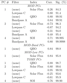
Table 2.2: Correlations between TOMS and MOD PCs and Various Indices
PC # Filter Index Corr. Sig. (%)
MOD PCs
1 (none) Solar Flux 0.26 84.3
Lowpass C 0.80 91.4
(none) QBO 0.80 99.91
Bandpass A 0.84 99.91
2 (none) Solar Flux -0.73 96.3
Lowpass C -0.87 94.2
(none) QBO 0.31 94.0
Bandpass A 0.48 95.4
4 (none) SOI 0.71 99.995
Bandpass A 0.80 99.9998
MOD-Band PCs
1 (none) QBO 0.84 99.8
MOD-Low PCs
1 (none) Solar Flux 0.84 95.8
TOMS PCs
1 (none) QBO 0.88 98.7
2 (none) Solar Flux 0.80 99.6
Lowpass C 0.95 99.91
3 (none) Solar Flux -0.25 93.6
Lowpass C -0.61 95.9
Table 2.3: Correlations between NCEP/NCAR Reanalysis PCs and Various Indices
PC # Filter Index Corr. Sig. (%)
NCEP-Layer PCs
1 (none) Solar Flux 0.43 84.6
Lowpass C 0.60 84.5
(none) QBO 0.20 86.8
Bandpass A 0.30 88.4
2 (none) Solar Flux -0.15 92.3
Lowpass C -0.50 84.1
(none) QBO 0.92 99.997
Bandpass A 0.94 99.9993
3 (none) SOI 0.82 99.9999
NCEP-100 PCs
1 (none) Solar Flux 0.22 83.5
Lowpass C 0.66 91.6
(none) SOI -0.43 96.7
Bandpass A -0.54 99.2
2 (none) Solar Flux -0.29 77.9
Lowpass C -0.40 75.2
(none) SOI -0.72 99.997
0.0
1.6
3.1
4.7
6.2
7.8
9.4
10.9
12.5
14.1
15.6
17.2
18.8
20.3
21.9
23.4
25.0
DU
<