Optimum linear coding for additive noise systems using information feedback

USING INFORMATION }i'EEDBACK

Thesis by Stanl ey .Butman

In ?artiaJ. FuJ..i'iJJ.ment of tbe Req_ui.rements

For the Degree of Doctor of Philosophy

Cal i fornia Institute of' Technology Pasaclen8. J California

ii

ACKNCWLEDGEMENT

The author wishes to than~~ Professor Thomas L. Grettenberg for his advice, guidance, and many helpful discussions prior to, and during the course of this work.

The research described in this report was conducted during the tenure of a Radio Corporation of America FeJ_lowship. Tne author is grateful for this assistance. A portion of this work was also supported by Naval Ordnance 'l'est Station, Pasadena Annex Contract No. N00123-67 -C-1188.

:- ABSTRACT

The feedback coding problem for Gaussian systems in which the noise is neither white nor statistically indep2ndent between channels is formulated in terms of arbitrary linear codes at the transmitter and at the receiver. This new formulation is used to qetermine a nwnber of feedback communication systems. In :particular, the optimwn linear code that satisfies an average power constraint on the transmit ted signals is derived for a system with noiseless feedback and forward noise of arbitrary covariance. The noisy feedback problem is considered

'

iv

TABLE OF CONTEN'IS

ABSTRACT iii

I. INTRODUCTION l

II. FORMULA'I'ION OF THE FEEDBACK CQvIMUNICATION PROBLEM. ₇

III.

IV.

V.

2.1. Introduction . . . 7 2. 2. Description of the General Linear Coding Procedure 7 2.3. Derivation of the Maximum Likelihood Decision Rule 11 2 .4. The Probability of Error . . 12 2.5. The Signal Selection P-.coblem 14 NOISELESS FEEDBACK . .

3

.1.

3.2. 3.3. 3.4. 3.5. 3.6.

3

,

7

.

3

.8

.

3,9,

3

.1

0

.

3.11.

Introduction . . . .

Selection of the Coding Matrix AB

General Form of the Transmitted S:ignals. General Sequential Form of the Receiver. Sequential Operation of the Transmitter.

Selection of g when the Noise is Uncorrelated. Optimwn Performance when the Noise is White. . Suboptimum Codes that Achieve Channel Capacity A Class of Codes that Achieve C for the

00

Additive White Noise Channel . . . . Signal Selection with an Additional Constraint Selection of g when the Noise is Correlated.

NOISY FEEDBACK . . . .

4.l. Introduction . . . . 4.2. Solution of the Signal Selection Problem 4.3. Selection of A and g when B =~I. .

4.4..

Evaluation of det(I+yAAT) and P-.cobability of Error . . . .

4.5. Selection of the Block Length . . . . 4.6. Mechanization of the Code . . . .

4.7

.

Selection of the Feedback Signals for a Specific

Set of Forward Signals 4.8. Discussion

RECURSIVE CODING FOR NOISY FEEDBACK. 5.l.

5.2. 5.3. 5.4.

5.5

.

5.6. 5.7.

Introduction .

Description of the Process . . . . Recursive Estimation at the Transmitter (Kalman Filtering) . . . .

Recursive Estimation at the Receiver Equations for P, Pfb' P and R Asymptotic Performance of the Code c

'I'he Wideband and Narrowband Rates . .

[image:4.558.66.475.64.684.2]

VI. CONCLUSIONS 86 APPENDICES

I. PROOF OF THEOREM II. . . 88 II. THE CRITICAL RATE OF A FIRST ORDER MARKOV CHANNEL

vi

LIST OF ILLUS11RATIONS

Figur~

l A Linear Feedback Communication System . . . . • 2 Matrix Formulation of the Feedback Communication

3

4

Process. . .

Bandwidth vs Coding Delay for a Class of Systems Feedback Coding with Recursive Estimation at the Transmitter. . . • . . .

7

9 30

I. INTRODUCTION

Two-way communication systems have the capability of transmitting

information about the current status of a message being decoded at the

receiver back to the transmitting point. The returned information can

be used to simplify the coding and decoding operations in the forward

channel and to :provide a lower probability of error for a given

coding delay than could be achieved without feedback. A potentially

useful application of information feedback is in the design of efficient

data retrieval systems for space vehicles, where the transmitting power

is restricted to be several orders of magnitude less than the

trans-mitting power of the ground based receiving equipment.

The analysis of a feedback communication system is similar to the

one-way communication problem in that it can be separated into a

decision or decoding probl.em and a signal selection. or codine; problem.

It differs only in the sense that in the coding problem it is possible

to optimize over both the forward and feedback signal sets. Previous

authors have approached the feedback communication problem by assu,~ing

a specific functional relat ionship between the feedback signals and the receiver~ estimate of the message, a functional form for the decision

procedure, and solving the remaining signal selection problem for the

:forward signal_ set. '111is approach [6,14,17,19] a..'1.d other methods [l-19] have succeeded in developing a number of efficient feedback communication

schemes, mainly for the additive ·white Gaussian noise (AWGN) channel with

a noiseless feedback link and the binary syrn_rn.etric (BS) channel_ with a

noiseless BS feedback path [J_3]. However, becau.se of the structm·al

remains to be determined even for the AWGN channel with a noiseless

return link. Systems in which the noise is not white have received

only passing mention. Attempts to take feedback noise into account

[l7,l8] by using a Kalman filter [20] at the transmitter have not used

an optimum decoding procedure nor an optimum set of feedback signals.

In this paper, the feedback communication problem for Gaussian

systems in which the noise is neither white nor statistically

independ-ent between channels is formulated in terms of arbitrary linear codes

at the transmitter and at the receiver. The maximum likelihood decision

rule, which is optimum for an equiprobable message source, is determined

and the signal selection problem is posed for both the forward and

feedback signal sets. This new formulation, is developed in Chapter

II, and is used to determine a number of feedback communication systems,

In Chapter III the optimum linear code is derived .for a system with a

noiseless feedback channel and an average power constraint on the

transmitted signals. The noisy feedback problem is considered in

Chapter IV where signal sets for the forward and feedback channels are

obtained with an average power constraint on each.

Chapter V considers the use of Kalman filtering at the transmitter

combined with an optimization at the receiver.

The present approach is valid for non-Gaussian systems provided

second order statistics are available, the results being applicable for

the determination of error bounds by such methods as the ChebycheV

3

The general formulation may be classified as a fixed-time-of-decision or block--codi~~L syst~ in opposition to sequential-decision

systems in which the time-of-decision is a random variable. This is the fundamental dichotomy which separates all of the feedback communi-cation systems reported in the literature, In each class, information feedback, if it is sufficiently accurate, can provide improved perform-ance. A special case of the latter category is when feedback is used to inform the transmitter only of the event that a decision has been

made so that a new message may be initiated. This has been generally referred to as decision-feedback and was studied by Bloom, Cha.ng, Harris, Hauptschein, Metzner, Morgan, Schwartz, and more recently by Viterbi

[5-9,12].

'l'hey consider the transmission of binary messages using signals that are also binary (two-levels) over the AWGN channel with a noiseless feedback l ink. Viterbi also considers the M-ary case and uses M ortho-gonal binary signals. He obtains exponential bounds for the error probability and shows that the negative exponent is four times the exponent for the best available error bound on the one way channel when the rate of transmission exceeds half the channel capacity.

Sequential-·decision systems using information feedback to

4

new signals are received and selects the message whose a posteriori

probability, relative to the other messages, is first to exceed a

threshold. The thresholds are set by the desired probability of

error. Continually returned feedback information allows the

trans-mitter to select signals that will maximize the a posteriori probability

of the message being sent and informs the transmitter when a decision

has been made.

The approach in [l4] and [l9] is based on the continuous time

channel and makes the assumption of instantaneous feedback. A binary

message source is used and the likelihood function (the logarithm of

the ratio of the two a posteriori probabilities) is continuously

computed from the received time function. The transmitted signal is a

linear function of the message being sent (0 or 1) and the current

value of the likelihood function available from feedback. The evolution

of the likelihood function is governed by a Langevin differential

equation which is driven by White Gaussian noise. Thus, the likelihood

function is a continuous Markov process whose probability density

satisfies a Fokker-Plank partial differential equation. A decision is

made the instant that the likelihood function first crosses one of two

thresholds. The time-of-decision, and hence duration of a message is a

random variable. The transmitted signals are constrained in peak and

average power and are chosen by Turin to minimize the average duration

of a message. The result is

5

The probability of error vanishes when the bandwidth is infinite and

the peak power constraint is rembved, so that a rate l

'T

nats/

second which is equal to the capacity of the infinite bandwidth AWGN

channel is achieved.

Horstein's earlier work [l3] on the BS channel is similar in the

sense that the nuniber N of binary channel symbols per binary message

takes the place of T. N is a random variable for which a bound on

the mean

N

is found as function of the rate R, channel capacity C

and probability of error Pe.

The operation of a block-system is based on the principle that the

number or block of signals associated with each message is a determin-istic quantity. The block length and the instants at which signals are

transmitted are known to the receiver. The receiver may compute the a posteriori probability over the message set either continually as

new signals arrive or after the entire block is received. However, the decision is made only after a complete block has been received so

that the decision time is deterministic and decision feedback alone is of no use. On the other hand, information feedback that is continually provided to the transmitter allows the transmitter to select signals

that will maximize the a posteriori probability of the message being sent. This approach has been used by Elias [10], Schalkwijk and Kailath

[15,16] and Omura [17] for the AWGN channel with noiseless feedback and

an equiprobable M-ary message set. Their results achieve the finite

and infinite ba.ndwidth capacity limit of Shannon [l] when an average

power constraint is imposed, but are not optimum because the coding in

[l5,16] is not optimum while in [17] the maximum likelihood rule is not

6

Although some authors evaluate the performance of their noiseless

feedback codes in the presence of feedback noise, procedures specifically designed to minimize feedback noise were not available prior to the

work of Omma and Kashyap [18]. They use a Ka.J_man filter at the

transmitter to fcrm the best estimate of the receiver's nstaten. However, the choice of feedback signals and decision procedure is not

7

II. FORMULATION OF THE FEEDBACK COMMUNICATION PROBLEM

2 .1. Introduction.

In this chapter the feedback communication problem for a system

in which the forward and return channels are both corrupted by additive

Gaussian noise is formulated using arbitrary J_inear operations at the

transmitter

and

at the receiver. This kind of an approach is applicable

to situations that are more general than systems with Gaussian noise.

However, the Gaussian assumption (and the assumption of linearity)

allows simple closed form expressions for the optimum decision rule,

and the probability of error, to be determined. In order to set up the

signal selection problem, the above expressions art::: augmented by

equations for the average energy transmitted in the forward channel and

the average energy required to send feedback information.

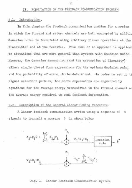
2.2. Description of the General Linear Coding Procedure.

A linear feed.back communication system usi.ng a sequence of N

signals to transmit a message

e

is shown below

s .=g.

e

+

l l

V.=U.+:r:J.. l l l

-Fig. 1.

i-l

n. l

r.=s.+n.

J.

z=l

al. J" v l.

4

l l l

- - -

---

+

>---- - - - Dec_rule ision

m.

l

i

.

l.:

b . . r .

lJ J

-Linear Feedback Communication System.

[image:13.553.43.491.45.682.2]

8

Only the discrete version of an additive noise channel is considered. The connection between the discrete and continuous formulations is wel l known [21-23] and will not be discussed further. The process begins with sl = gl

e

being transmitted, rl = gl

e

+ nl, being received,, u

1 = b11r1 is the first feedba,ck signal which is observed at the re-ceiver as The next signal to be sent can be a linear function of

e

and _vl' and is thus written as

The general term is

i-1

s . = g

e

+

I

a .. v.

l l lJ J i 1, 2, • • • , N (2.1) j=l

and

i

u.

I:

b .. :r.

l 1.J J i

=

1, 2, • • • , N-1 (2.2)

j=l

The last, or N-th, feedback signal is not used in and is therefore not fed back, nor is it generated.

It is convenient to write the above and remaining analysis using vector and matrix notation. Therefore, let s = col(s_{1, s2'}

..

.

_sN)'

'

r = col(r

1,

...

'

rN), u col(ul' u2,

'

., VN ) ' v = col ( v 1, v2' vN)' n = _{col(np n2'}

...

_nN)' m - col(m

1, m2' ~),

g col(g

1, g2'

..

.

'

gN, '\ and let (A) ij = a .lJ' . , (B) l..J .

=

b .. be lJ N x N lower trianguJ.ar matrices with the ma.in diagonal of A and the N-th row of B identically zero. Then

9

u =Br (2 .3)

v u + m (2.4)

s g8 + Av (2.5)

r s + n (2. 6)

Note that A anihilates the N-th component of v

'

while the zero N-th

row of B causes ~ to be zero as required. The system is now

equivalent to the N-dimensional vector channel bel ow

n

s .

Decision l=============rr==::::::~ rule

r

A

Fig. 2. Matrix Formulation of the Feedback Communication Process.

*

... 8

Now l et m and n be jointly normal with zero-mean, covariance

K _m and K _n , and cross-covariance Kmn' where K = E[rnm T ],

m T

Kn =. E[nn

J,

K _mn E[mnTJ and E[·] is the expectation operator

whi le 11

T" denotes transpose. The conditional p:cobabil i ty density

p(r/8) can be found after r is writ ten as a function of the random

variables

e

,

m and n. This is done by substituting (2.4) into

(2.5) and the result into (2.6)

10

The conditional mean E[r/8] and covariance E[(r-E[r/8J)(r-E[r/8])T/8]

are respectively

(2.8)

and

K = (I-AB)-l K(I-AB)-T

r (2.9)

where,

K = AK AT + AK + KT AT + K

m mn mn n (2.10)

Then

(2.ll)

(2.12)

where det K

= det K because det(I-AB)

is unity, a result that

r

follows from the fact that AB is l ower triangular with zeros along the

main diagonal so that I - AB is lower triangular with ones down the

11

2.3. Derivation of the Maximum Likelihood Decision Rule.

In general, the optimum decision procedure for minimum error is

the ideal observer rule. The procedure is for the receiver to select

the message that maximizes the a-posteriori probability distribution

p(8/r). If p(8) is the a-priori probability distribution on the

message set, then Bayes' rule gives

p(8/r) = p(r 8)p(8)

P r . (2 .13)

When 8 is equiprobable over a finite set of M real points,

p(e)

= -

l then M '

p(e/r)

=

p(r{ej

Mpr

(2.14)

Maximization of p(8/r) is equivalent to maximization of p(r/e),

which is the maximum likelihood rule. p(r/e) is maximized over e if

and only if \\r-r 8

!1

2

_₁ is minimized. Let

SN

be an arbitrary scalar K

r

\\r-r ₈112 _{_1} K

r

\\r-Au

-

ge

\1

2_

1

K

=

ll

r-Au-geN

+

g

(

eN

-

e)\\:_1

\\r-Au-

g

eN

\

\

2

_

1

-

2

(

e

N-8) (

SN\\g\\

2

-l

K K

The middle term drops out if I\ 9N is chosen to be

Therefore

\\r-r

e

1\2 -l K

r

12

(2

.

16)

(2 .17)

"

Since eN can take on any value on the real line while e is only one of a set of M discrete points) i t is now obvious that choosing e

closest to I\ _{eN max}imizes p(r/ e) over

e

.

This is the maximum like

-*

lihood estiJnate of e and is denoted by e it of course runs only

over the finite set of M message points. It is easy t o show that

"

eN is in fact the minim1..un-variance unbiased l inear estimate of e. "

The conditional mean and variance of eN are

e

1

ll

g\\2

_l

K

2 .L~. The P-.cobab ili ty of Error.

(

2

.1

8

)

(2

.

1

9)

An error occurs at the receiver each time

e

is transmitted but

e*

f

e, that is,

I

eN

.

.

e

I

is not a minimum. If the M equiprobable

messages are equispaced on the interval [-L,L] on the real line, the nearest neighbor distance is

I./(

M

-

1

)

and tbe condition for an error

1

3

[-L,L]. If

e

is one of the end points, ± L, the condition is

eN-8

~

+

L/(M-l)

respectively. The conditional error probability for

e

f

± L is Pe = pr(leN-el

~ M~

1

/e}.

Thus,

where

and,

P

0 • l -

f

p(9N/e)

1eN-

e

1

s;

L/(M-l)

30e2

ll

gll2

_1

K

00

erfc x

=

~

J

e-x

2

dx

-Vx

x

oe

2 = E[82]

L2

(M

+

l)

=

3(M-l)

(E[eJ

=

o)

(2.

20)

(2.

2l)

(2.

22

)

(

2

.

23

)

( 2 ~24)

When

e

is one of the end points, P is slightly lower but negligibly

e

14

2.5. The Signal Selection Problem.

The signal selection :problem is to choose A, B e.nd g to

minimize P subject to constraints on the forward and feedback e

signal sets. Important constraints are the average :power in the for

-ward and feedback channels, or equivalently, the average energy :per

transmitted message in the forward and feedback channel s.

N

E == E

L

s.

2

1 av

i=l T

== E [Tr SS ]

(2.25)

== Tr[(I-AB)-1c0

8ggT + AKmAT + 2AKmnBTAT + ABKnBTAT)(I·-BTAT)-l]

(

2

.

26

)

and) since

e

is statistically independent of n and m)

where

Let

N-l

E == E

fb

I:

i=l 2 u.

)_

== E[Tr BrrTBT]

Tr[.

J

is the trace

N 2'1W where T

(~ - o)

N

operator defined by Tr[Q] ₌₌

l:

i=l is the duration of the message,

(2.27)

(2

.

28

)

CJ.ii.

or coding

delay, and

w,

which is defined here to be N/2T, is the "bandwidth"

of the forward channel. Note that the t ime duration of the (N-l)

feedback signals is 2W/(N-l) so that the average power in the forward

while

p == 2W E N av

2W

pfb == - -_N-l E _fb

is the feedback power.

15

(2.29)

(2.30)

other constraints may be either substituted for, or added to, the

above conditions. Since erfc x is a monotonically decreasing function

of x, minimization of Pe is equivalent to maximization of

0

8

2

\\g\\2 _₁ and hence

16

III. NOISELESS FEEDBACK

3.l . Introduction,

This chapter presents a number of new and interesting results for noiseless feedback systems. Primarily, the sequential form of the

optimum operation of the receiver and transmitter is derived for a

general forward covariance matrix. Secondly, Theorem 2 proves that it is possible to achieve capacity for the wideband and finite bandwidth

AWGN channel in an essentially uncountable nwn"ber of non-optimum ways. Thirdly, it is shown that Schalkwijk's scheme follows from the solution

of the signal selection problem with additional constraints. Fourth, it becomes evident thg,t the dynamic programming approach of Omura, for

which it was necessary to assume the functional form of the receiver, uses the optimlun signal set, but not the optimum decision rule. The

discrepancy disappears in the limit as the block length goes to infinity

because the minimum variance estimate is asymptotically unbiased.

Finally, an almost optimum.code for a chan~1el with first order Markov noise is obtained. The critical rate of this code achieves the

theoret icaJ_ capacity when the bandwidth is large, and almost the capacity

when the bandwidth is finite.

A model that assumes a noiseless feedback channel may be used to

represent a system in which the noise in the :forward channel predomin-ates. Calculations based on this assumption are valid until the

cumulative effect of the small f'eedback noise becomes comparable to the

forward noise.

The absence of feedback noise is reflected in the general formula

-tion by the vanishing of the noise vector m, the covariance K a..11d

17

the cross-covariance K .

mn As a result, eq_uations (2 .lo), (2. 26) and

(

2

.

28)

simplify to

and

K = K

n (3 .1)

(3. 2)

(3 ,3)

However, can be arbitrarily small for any choice of E and av

P , because

e B may be scaled d.own to EB while A is scaled by

l

E Thus, the product AB remai.ns unchanged, E _av is unaffected,

l\gll

2

_1

and hence K

p

e is not affected, but Efb is scaled down by

2

E

which can be made arbitrarily small. The signal selection problem for

the noiseless feedback case is therefore not constrained by feedback

eq_uivalent to minimizing E for av

\lg\\2 _₁ for a fixed value of Eav

K 2

fixed \\gl\ _₁. Note that only the

K

is power. The problem of maximizing

product matrix AB and g need be found. When there is feedback noise

it will be necessary to solve for both A and B.

3. 2. Selection of the Coding Matrix AB.

Let I + C = (I-AB )-l then C = ( I-.A.13 )-1Jl...B = AB (I-AB )-l is lower

triangular with zeros along the main diagonal, note that AB

=

C(I+C)-1•

E

l8

The N(N-l)/2 non-zero elements of C are _arbitrary because the

N(N-l)/2 non-zero elements of AB. are arbitrary. Tne constraint on

\\g\\2 -l does not affect the choice of C7 therefore7 the minimization

K

over the elements of C can be performed using ordinary calculus for

all values of g. Subsequently₇ when E is found in terms of g₇ av

its optimization over. g will have to include the constraint \\gl\2 -l '

K

Let c(i-l) == col( cil; ci2' ,. c. _{l l -}. ₁) denote the first i-l elements of the i-th row of C₇ .the remaining elements in the row are

zero because of the lower triangular zero-diagonal form of C. Also,

let

...

then

N

Eav

L

[o 9

2

(gi + (c(i-l),g(i-1)))2 + (c(i-l)K(i-l)c(i-l))]

where

n. l).

l

-K(i-1) == Kn(i-1) == E[n(i-l)nT(i-l)], n(i-l) == col(n₁,

2

Note, that the individual signal energies, e. == E[s.]

l l

given by

(3.5)

n •••

2' '

are

ei == o₈2(gi + (c(i-l),g(i-l)))2 + (c(i-l)K(i-l)c(i-1)).

(3.

6

)

Now, setting grad E

c(i-l) av

r, . ...:,.· 0

.\".j

for i _{2, 3, · · · , N} (c(l)

=

0) gives

c(i-1) == - o₈2(gi + (c(i-l),g(i-l)))K-1(i-l)g(i-l) . (3 .7)

Taking the inner product of both sides with g(j ... 1) and solving r~or

(c(i-l)7g(i-l)) in terms of gi and \\g(i--J_)\\2

19

2

c(i-1) ==

0

e

gi l

- - - K- (i-l)g(i-1) .

Therefore,

and

2 2

0

e

_gi

e. ==

-1 l + cre 21\g(i-l) \\2 -l

K (i-1)

N

i == l, 2, • • • ' N

(3 .8)

(3.9)

E = \

av

L

(3 .10)

;!.· ,., .... •'

,, , •,,r It remains to minimize E with respect to g which is constrained

av

by

l\gl\2

_l .

K

This is accomplished by setting

and solving the resulting N non-linear e~uations for the

The solution when K == K is diagonal is straight forward and is

n

available in closed form. When K is not diagonal the problem is more

involved. However, it is not difficult to obtain a good, although not

necessarily optimum, choice for g. Also, the functional form of the

transmitted signals and a se~uential form for the computation of

"

e

N

at the receiver can be derived without knowledge of g.

3.3. General Form of the transmitted Signals.

From s == (I-AB)-l g8 + (I-AB)-lABn == (I+C)ge + Cn it follows that

si+l == (gi+l + (c(i),g(i)))e + (c(i),n(i))

Since r-Au = g8 + n, the minimum variance unbiased estimate of

e

after N observations is obtained from

(2.16)

as

and after i observations it is

The ref ore

Define

then

(g(i),K-1(i)n(i))

llg(i)\\2 1

K- (i)

gi+l (

e

-oe2\\g(i)\l2 l K- (i)

1 + oe2l\g(i)\\2 1

K- (i)

082\lg(i)\\2 -1

K

(i)

/\

e.

_l

l + cre2\\g(i)\\2 _1 K (i)

is the desired result.

(3 .12)

(3

.13)

(3 .14)

(3,15)

(3.16)

There is no difficulty in showing that x. is the minimum

l

variance linear estimate of 8 given the observations r

1, r2,

Note that xi is a biased estimate (E[xi]

f

8) as opposed to the

estimate e. /\ which is the minimum variance unbiased estimate.

3.4.

General Sequential Form of the Receiver.

The positive definite symmetric covariance matrix K may always

be factored into the product K

=

QQ.T, where Q is lower

tria.~gular

and positive definite. Similarly, K(i)

=

Q.(i)Q.T(i) where Q.(i) is

the upper le~ i x i

g(i) = !_ Q.(i)f(i)

ae

and

corner of Q.. Let g = -l Q.f,

oe then

\\g(i)l\2 =

·

~

\\f(i)\\2 where

K-l(i) oe2

...

, fi). Then

= llr(i-l)\\2

e

+ o

9 (±'(i-l)Q.-1

(i-l)n(i)) + fi2

e

+ o

9fi (h(i),n(i)) (3.l7)

where h(i) = col(hil' hi₂, • • • , hii) denotes the i-th row of Q , - l

. ( -l)

that J_s h .. = Q . . for j =:;; i = l,

1J 1J 2, • • • , N. Thus,

\\r(i)\J2

e

.

=

\\f(i-1)\

\

2

~.

l + f.(f.e + (h(i),n(i))) .

J_ 1 - J_ J_ (3 .l8)

But therefore

(3.19)

But, recall that

~

+ \\f(i) \\}i == l\f(i)\\2

ei'

therefore,

(l + l\f(i)\\2)xi = (1 + \\f(i)\\2)xi-l - fi 2xi-l + o₉fi (h(i),(g(i)e + n(i) ))

Since g. ( 8-x. l)' J

J-22

i

\ h .. (g.8 + n. - g.x. l) .

L__, lJ J J J

l-j=l

r.

J s . J + nJ . becomes

g . 8 + n. = r . + g .x . l '

J J J J

J-i t follows J-immedJ-iately that

i

h .. [r. + g.(x.

1-x. l)J .

lJ J J J-

l-(3.2l)

(3.22)

(3.

23)

The above resu_lt is valid for any positive definite covariance

matrix. In particular, when the noise is white so that K = 021,

- l l l 0

e

Q

0 I, hij

=

cr

6ij' f

=

0-

g i t reduces to

(3.24)

If the noise is generated by a first order difference equation

ni

=

ani-l + wi' where wi is white noise with covariance

then Kn= (I-aJ)-lKw(I-aJT)-l where Jij = oij+l" Thus

so that o h(i) = col(O,

o,

, o,

-ex,

l). Then

w

2

K

=

o I,

w w

-l 1 ( '

Q I-aJ J

0

w

082(g.-ag.

1)

l l

-02 + llg(i)-ag(i-l)ll2

[r.-ar.

1 + ry.g. l(x. l-x. 2)J

l l - l - l - l - (3.25) w

23

noise obeys a linear difference eg_uation of order m which is driven by white noise, then the minimum variance estirno,te obeys a linear

difference equation of order m + 1. I\

The decision rule req_uires eN. It can be computed from xN via

the relationship eN = (l + \\f\\2)xN/\\f\\2, or

oe 2\\g\\2 -1

A K

9 _{= - - - 2 - -2- xN •}

N l + oe

\\g\I

- l K

(3.26)

The coefficient of xN approaches unity as \\g\\ 2 _₁ goes to infinity K

with N, and xN is asymptotically unbiased.

3. 5. Sequential Operation of the Transmitter.

Since the transmitted signals are related to the minimun1 variance estimates according to s. =

]_ g. ]_ (e-x. ]_-1) it fol.lows that x_J-. l-x_{i -}. l

=

s. ]_ s]_ .

Substituting this into the general formula for x.

]_

gi+l

s _i+l - - -_{- g.}

]_

gifi(h(i), (r(i)-s(i))) )

l + a e 21\g(i-l)\\2 -l

K (i-1)

:::

giei+l

gi+l ei ei (h(i), (r(i)-s(i))))

which reduces to

y

e.

1 (

e

.).

(

= J.+ - 1 + ~ Si

e. a J

]_

(3. 27)

3

.

6

.

Sel ection of g When the Noise is Uncorrelated.

If the noise is statistical ly independent between signals) the

covariance mat rix K and therefore also K is diagonal. The

n

diagonal elements are: k.J.

=

E[n.n.]

=

0 . 2 6 . ..

1 1 J 1 1J

then

But

e. 1

- 2 =

0. 1

f.2

1

l + \\f(i-1) 1\2

i

Let

l + [[f(i)\\2

-n

j=l (

l + \\f(j)\\2 )

l + \\f(j-l )

1

12

C

\

\

f

(

o

)

\

\

2

=

r

0 =

o)

=

n

i ( l + - - " " ' "

r.

J _ _ _

2

)

j =l . 1 +

\If

(

j -l ) 112

hence also

ei+l f r (l + ej )

2 . l 2

0e J= 0j

and

2 2 N ( e. )

1 ₊ 0

e

\J

g

l\

_{-1 =}

n

_{1 +}

~

K 1=1 0.

1

(3.28)

(3.29)

(3 .30)

(3 .31)

25

Therefore, the constraint on l\g\\2 _₁ is now a constraint on the signal

K 2 2

energies. I t is convenient to use ln(l + ere

j\g\\

_

1) and to set K

N

where

I

e. E av'

J_

i=l

e

vln(l + i ₂)

J

= 0 er.

J_

and \) is a Lagrange _multiplier.

E

av + Tr K

2 _i

1, 2, N

e. + er. \) =

...

N

'

J_ J_

The above condition is meaningful only if e. _{J_} = \)

-

er. 2

J_

situation that does not always prevail. If \)

-

er. 2 ::;; ₀ J_

.

(

3

.

33)

The result is

(

3

.

34

)

>

o,

a

the answer

is to set e. = 0 (thus also s. = O), N = N-1 and recalculate \)

J_

Assuming that this does not N

. J_

occur (E sufficiently large or

av

2

er. J_

~

Tr

1 NO

let K

='N

L

er. 2 = er 2 _{= 2}

N J_ Then, since E "" PT and N 2WT

i;::l

(

p 2WT

1 + - )

NW

N

2

TT(~)

i=l er. J_

(

3

.

35

)

0

( p ) 2WT

~ 1 +

-NW

0

3

.

7

.

Optimum Performance When the Noise is White.

If the noise, in addition to being uncorrelated, is stationary

N N

then kij = kj i-j

I

=

er2 6ij

=

₂

°

1\j'

where ₂

°

is the two-sided noise

power spectral density of white noise. Then

2 2

l + ere

\\g\\

-l

K

_R__)2WT

(i

+NW

0

and

where

p

e erfc

26

p

c

= W ln (l + N W) nats/sec 0

is the theoretical capacity of the channel and

l

R =

T

ln M nats/sec

is the rate of the message source.

By the v1ell known properties of erfc,

lim P

=

T__,co e

0

erfc}

2

1

R<C

R

c

R > C

The asymptotic behavior of the error is

p e

2

= - - e

3"\f

- J

e2(C-R)T + (C-R)T

2

(3 .38)

(3 .39)

(3.40)

(3.41)

(3.4

2

)

The double exponential decrease of the error as a function of coding

delay T, or block length N, is characterist ic of codes using

27

length due to a larger effect ive input alphabet then this resul t was

predicted by Shannon

[4].

3.8. Suboptimum Codes that Achieve Channel Capacity.

There is an uncountable suboptimwn choice of the signal energies

that allows corrnnunication at a positive rate, in fact, up

to channel capacity. Define

R (N)

c

Therefore

Theorem l

l

2T

N _e.

2=

ln(l +

~)

i=l 0

N e.

I

ln(l +

~)

i=l CJ

3

2

N e.

L

2: . l 2

1= CJ

e 2R T

c

- l

2RT

e - l

(3.43)

(3.44)

A necessary and sufficient condition for achieving zero error

for

Proof'

thus

0 <R < (l -o)R

c

N

L

2: e. ~

2

i=l 0

N

[

is

~E

2 av

CJ

=

co _{This is} an obvious condition.

e. N e.

ln(l + 2:) ~ ln(l +

L

-~)

2 . l 2

But p

e

E

E

av ;:z: R T ~ ln(l + av)

02 c 02

is zero in and only if

28

R T = 00_, thus c

E

av 02 =

(3.45)

oo e.

2=

~

=

00 . 1 2

J.= 0

Definition

Let R ( oo)

c be the maxim.um rate at which zero error can be achieved.

It is defined here by the two condit ions: (a)

~

L ei -- 00 , and

. 1 2 (b)

N e.

2=

in(J_ + ~)

i =l (J

J.= (J

R ( oo)

c

1. p

== J.m - -2

~00 20 N e.

2=

~

i=l (J

(3.4

6)

Theorem 2

If the sequence r_~ e.}~ l

J. J.== converges to a l imit then R ( c oo) is given

by

(a)

~

=

Wln(l + - ) p if lim e. p

NW NW

i-iro J.

p 0 0

R _c ( oo) (b)

c

₀₀

=N

if lim e. 0 (3 .47)

J..

0 i->oo

(c) 0 if lim e. 00

i-icc J..

The proof is in Appendix I.

3,9, A Class of Codes that Achieve C for the Additive White Noise CP

Channel .

Theorem 2(b) indicates that there exists a variety of feedback

codes that can achieve the infinite bandwidth capacity limit

method of classifying these schemes is to examine how NJ or

p

N

0

w}

One

29

signal energies are of the form

e == (2:)Y

i 1 (3.48)

where 0 ~ y ~ l. First, y == 0 corresponds to the optimum scheme in

which P/w == J., Cw == ln 2 so that W is finite and independent of T.

The other extreme is for y == l which gives

2R T

c _{- l}

therefore

2R T

W ==

(e c -

l)/2T

When 0 < p < 1 and T is sufficiently large,

thus

N

RCT ==

L

ln(l + i-y)

i==l

N

I:

i-y

~-y

l - y

for large N

(3 .49)

R ~ C

and

l l

N ~ [2C (l-y)Jl-y Tl-y

0 )

30

(3.50)

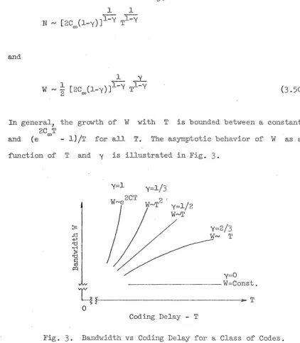
In general, the growth of W with T is bounded between a constant

2C₀₀T

and ( e - l) /T for all T. The asymptotic behavior of W as a

function of T and y is illustrated in Fig. 3.

Y=l _y=l/3

W ~e 2CT

Y=l/2

w~

y=O

~~~~~~~~~~~W=Const.

L~~~~~~~~~--T

0

Coding Delay - T

Fig. 3. Bandwidth vs Coding Delay for a Class of Codes.

3.10. Signal Selection with an Additional Constraint.

The coding scheme of Kailath and Scha:;_kwijk can be derived by

solving the signal selection problem subject to an additional constraint

_,

I

on AB, or C = (I-AB) -AB, and g. In their scheme, E[sl e]

=

gle

while E[s ./8] -· 0 for all i > 1. In vector form this translates into

[image:36.560.54.477.54.538.2]

31

setting E[s/e]

=

E[(I+C)ge + Cn/eJ = (I+C)ge

=

col(g

1

e,o, ··· ,

o).

Thus there is the auxiliary constraint (I+C)g = col(g₁,

?, ••• ,

0) or

g. + (c(i-l),g(i-1)) 0

. 1 i = 2, 3, • · • , N •

(3.51)

In

the white noise case considered by Schalkwijk, the present formulation gives

E _av

II

(I+C)gll2 ere + 2 o2Tr CCT

(3.5

2

)

N

'

2 2 ()2

I:

llc(i-l)l\2

ere gl +

(3.53)

i=l

The minimization over c(i-1) must now include the N-l constraint equations, which are easily incorporated via Lagrange multipliers

N N

2 2 ,.,.2

F

=

er

9 g1 + ...,

I:

l\c(i-1)\1

2

+

L

A..(g. + (c(i-l),g(i-1)))

1 1

(

3

.

54

)

i=2 i=2

and set gradc(i-l) F = 0 for i = 2, 3, • • • , N in order to obtain

A..

c(i-l) - ~ g(i-1),

2cr

(3.5

5)

hence,

i 2, 3, • • · N (3.56)

2 = .CY2 _ _

g_i_--,,-1

lg (

i-l) \ \ 2

Next, note that

therefore,

while,

N

E =

I:

av

i=l 2

CYe 2

= - g

CY2 l

e.

1

32

2 )

N g.

n

l + 1 2

h2 ( [[g(i-1)[[

The optimum choice of signal energies is

2

E -CY

av

N

2

- CY • Therefore,

(the optimwn result)

(

3

.5

7

)

33

with equality when N

=

1 and of negligible difference as N

in-creases. However, in this case e

1 exceeds the remaining e's by

2

cr .

If all the signal energies are made equal, the result is

(

- )N-1

cre

211gll

2

-1

=

E

~v

1 +

Ea~

K cr N Ncr (3.59)

p

which is considerably less than

E

)

N

(1 +

~

_Ncr2 when

E

av

Ncr2 NW is small.

0

The form of the transmitted signals is obtained by eliminating

c(i-1) from the expression for s.

]._ as in Section 3.3. The result is

/\

s. = g.(e-e.

1).

]._ ]._ ]._

-2

Similarly, it is easy to show that A

e

]._

.

-1 +

gicr

is the sequential operation to use at the receiver.

3.11. Selection of g When the Noise is Correlated.

The problem of optimizing E

av over g when is fixed,

is in the case of correlated noise complicated by the non-diagonal

nature of K. The problem appears to be formidable even in the case of

a simple first order markov process. It is not difficult, however,_ to

guess a good g and to compute the resulting performance. The

defini-t ion for R is still gi~en by

c

R

c (3.60)

Factorization of K into the product QQT where Q is lower trianguiar

and.positive definite, and setting

1 +

ae

2\lg\12 -1 = 1 +

llrll

2. The identity K

g 1 Qf,

l +

\lf\1

2

l +

can be used to obtain

However,

R =W.:!:

f

ln(l +

c N i=l 1 +

E

av

N

2=

(f(i),q_(i))2 i=l"l + \lf(i-1)112

f. 2 )

\\f~i-1)

\\2 .

is not simplified. Here, f(i) = col(f

1, f2_,

(3. 6l) .

(3 .62)

(3. 63)

col(q_il' q_i₂' ••• , q_ii) is the i-th row of Q, and the individual signal energies are of the form ei

=

(f(i),q_(i))2/(l + l\f(i-1)\\2).

Thus, there does not exist a simple relationship between y.

=

1

f. 2/(l + llf(i-·1)112) and e. as in the case of a diagonal covariance

1 1

matrix. Nevertheless, at least two good guesses are available. The first is to let y. = y a constant independent of i . This gives

1 .

R _c = W ln ( 1 + y) (

3

.

64)

and

-J

(

i-l

±f'. = y ,1 + y)

1 (3. 65)

E

av

35

Note that the sign in front of each

(3. 66)

f. affects the terms in E but

i av

not those in R where the f. appear squared. This allows a partial

c J.

minimization of E over sgn f. to be carried out.

av J.

The second guess is to maintain constant average power by choosing

all the e. 's equal to a constant, say e.

J. Then

E _av == Ne

and

(3. 67)

where h(i) == col(hil' hi₂' • • • , hii) is the i-th row of Q.-1,

g. ==

~

(q(i),f(i)), and f

1. = 08(h(i),g(i)). Once again the signs of

i

cr

e

the components in the inner product are avaiJ_able for partial

optimiza-tion of R . An example for the case of first order Markov noise is

c

worked out in Appendix II where it is shown that for both yi = y,

and e.

=

e

l

p

NW

0

'Y

(1 . T~

~)

36

where

ex

is the :Parameter of t he Markov noise The critical rate achievabl e is then

R

=

W ln(l + l') c

p

. W ln(l + NW) 0

(l +

j

exj

)2 NPW 0

for __!._ >> l NW

0

f'or ~ << l

NW 0

(n.

=

an.

l + -w.).

1 1 - 1

{3.69)

(3. 70)

·-where N

0

2

is the spectral power density of the white noise which

drives the dif'ference equation to produce Markov noise, N

(E[ w. w.]

=

2

°

6 .. ) •

37

IV. NOISY FEEDBACK

4.1.

Introduction.

The inclusion of feedback noise is essential in the representation

of a physically realizable system. otherwise, as it is shown in Section 3,l, it would be possible to use arbitrarily weak feedback signals for

conveying information to the transmitter. Thus, in the case of noisy

feedback, the probability of error is determined by the feedback power as well as the power used in the forward channel.

The main purpose of this chapter is to establish the relationship

between the forward and feedback power and the probability of error for systems in which the :10ise in the forward and feedback channels is 1,-;hite .

and independent. There are many pr a.ct ical s i tuci.tions in which this assumption is valid. Thus, if

forward and feedback noise, then

N

where a2 :::: 0 is the two-sided

2-forward channel and y == a ·2

/o .

2

m

2 T

K == er (I + yAA ) ,

2

and 2 the variances of the

a a are

ID

K a I, 2 K ya2I and K _-·

o,

n ID mm

noise power spectral density in the

Equation

(

2

.10)

simplifies to

(4.l)

and, letting I+ C

=

(I-AB)-1, where C == AB(I-AB)-l is lower tri-angular with zeros along the main diagonal allows

(2.29), to be written

E

av' as given by

38

However,

Tr[(I+C)(I+C)T - C - CT - I] (4 .3)

and Tr[C]

=

0 because the diagonal elements of C are identically zero. Also Tr[I]

=

N; therefore

Substitution of (4.4) into (4.2) produces

E

av

N 2 + E

0 av

2 T 2 T 2 T 2

Tr[(I+C)(oe gg +om AA +0 I)(I+C)

J

-

0 N

2 T T

Tr[(I+c)(oe gg +K)(I+C) ]

Note that the above simplification is possible only because

(4.4)

(4.

5

)

(4

.6

)

K was

n

assumed to' be diagonal. The feedback energy as given by equation (2.30)

may also be written in terms of

c,

2 T T T

Tr[B(I+C)(oe gg +K)(I+C) B

J

(4.7)

Finally, the quantity that controls the probability of error is

l

(4.

8)

39

It is easy to see that the simple scaling argument B _. EB,

1

A _. - A E '

AB_. AB of Section 3.1, that caused E:fb to be arbitrarily

smal l without affecting E _av and llg\j2 _₁ fails; because, in the

K 2 T

present case K =

a~(I+yAAT)

becomes a (I +

Y

2 AA ), thereby E

causing jjgjj2 _

1 to decrease while

K

E

av increases as E is reduced.

A more subtle but equally unrewarding pursuit is to choose g in

the null space of AT. This choice is deceptively promising but it is

easy to prove that it leads to the no-feedback solution A

=

O. First,

in order to show why such a choice is seemingly good, note that

K-1 = 12 (I+yAAT)-1

a

therefore,

= 12 [I-yAAT(I+yAAT)-1] ' a

jjgl\:-1 = : 2 \jgj\2 - y(g,AATg) K-1

~

~

\lg\\2

02

(4.10)

(4.11)

(4.12)

with equality if and only if ATg

=

o.

Thus it seems that

E[(eN-e)

2

/e]

and the probability of error, are minimal and independent of the feedback

noise when ATg

=

O. Since the rank of A is at most N-1, there

4o

Now, in order to prove that this condi:tion leads to the no

feed-back case A

=

0 as the optimu.~ solution, consider the expression

for · E as given by (4.2).

av

E av

2 T 2 T T 2 T

Tr[(I+C)(ae gg +am A . .A.. )(I+C) + a cc ]

ae2(\\g\l2 + 2(g,cg) + l\cg!l2) + a2(y\!(I+C)A\]2 + \lc\\2)

:2'. 0 _e2_(\\gl\2 _{+ 2(g,cg))}

t ( -- )-1

Bu C ::: AB J_-AB , therefore

(g,

c

>

g

T ( )-1

g AB I-AB g

vanishes when gTA (A T T g) = O. Thus, if A T g 0 then

(4 .13)

( 4 .11~)

with equality if and only if A

=

O. In fact, the only ~uantity that

can -become negative, and thereby play a I112.jor role in minimizing E ,

av

is (4.14). This impl ies (without proof, however) that A and B

should have, as in the noiseless case, rank N-1, which is the maximum

4l

4.2. Solution of the Signal Selection P-roblem.

An important relationship between E

av' E fb and for

systems with white and independent noise can be established by the use

of several well known matrix: properties. Let

~

-l 0

e

T T T T -l

(

2 )

~ = (I-.P.B) <J

2 gg + I + yAA (I-B A )

(4.l

6)

Since AB is lower triangular with zeros dovm the main diagonal,

I - AB has ones d01m the main diagonal and det (I-AB )-l = l.

There-f'ore,

det H det(I-AB)-2

det H

(Je

( 2

det · -02

T

gg + I+

. (4.17)

where, in general, det(I+xxT) = l + llxil2 for any vector x. The proof of this fact is simple. The vector x is itself an eigenvector

T T

x(x,x)

(l

+

llxl\

2

)

x.

of the matrix: I + xx becau.se (I+xx

)x

x +

=

Thus the eigenvalue associated wi th x is l +

!\x\1

2• Since I+ x...x T

is synnnetric the remaining N-l eigenvectors must be orthogonal to x.

Thus, if y is any other eigenvector, (x, y)

=

o, and (I+xx T )y

=

J,

proving that the remaining eigenvalues arc al l equal to u.""lity. Since

the determinant is equal to. the product of the eigenvalues, the proof

The result for 1 +

42

oe

2llg\12 .. 1 K

is obtained by letting

T T

QQ = I + yAA and

Q(xxT + I)Q.T. Thus

0

e

-l x = 0 Q g,

(

2 0

e

T

so that

02 gg + I +

det H

det(I+yAAT)

N

n

\I.

i=l l.

= - -

-det(I+yAAT)

where v

1, v2, •·· , vN are the eigenvalues of H. Also

E

N+ _-2-av Tr H

0

N

=

l:

\ ) . 1 i=l

and

(4.18)

(4.19)·

(4.20)

where Tr[BTBH]

=

Tr[BHBT] follows from the invariance of the trace

operator under cyclic permutations of the matrices .

Since erfc x is a monotonically decreasing function of x, the

minimization of P given E and Ef'b is equivalent to maximizing

e av.

subject to constraints on E

av and But, since

with

with

n

_i=l \I. s

J._

eq_uality if and only if \I.

J._ 1

=N

E

r

1 +

ae

21\gll2 -1 s

( 1 +. N:; ..

T

K det(I+yAA ) N

L'.

\I. = \I _{for al l} i=l J._

eq_uality if and only if all of the eigenvalues of H

(4.21)

i, Thus,

(4.22)

are eq_ual, that is, vi

=

\I

=

(1 + P/N

0W). In order to achieve the upper bound

. T

it is necessary to hold det(I+yM ) fixed while varying AB and g. Since every symmetric matrix whose eigenvalues are all the same is

a

multiple of the identity. matrix, H = VI ,

Note that (4.22) immediately provides the solution to the noise -less feedback problem (y=O) in which the forward noise is white.

The condition H

=

vI may not be achievable for some choices of B or A even if of rank (N-1). However, if i t is achieved then the

best choice of B (from the set for which H

=

vI) can be found as follows:

Efb

= 02 Tr

[BTBH]

(4

.

23)

N-1 N-l

\I

L I:

b~j

i=l j=l

N-l

\

b~.

> 0

L

11

i=l

44

Therefore, if the last row of B is disregarded because it is iden -tically zero, the determinant of the resulting (N-1) x (N-l) matrix

must be positive. Let _~l' 2 _~2' 2 ,

~;_

1

,

~

2 be the eigenvalues of l N2 N-l 2

Efb

-2

then _...,N P.

= v Tr[BBT]

i = 1., 2 • • • .

'

'

is identically zero, and ~- =

2:

b .. > O. Since

J._ i=l J._J._

=

~~'

it is minimized by choosing

~~

=

~

2 for all

N-l. This immediately indicates that BTB

=

~

2

L

_

J\r-l

where IN-l is the (N-1) x (N-l) identity matrix. Therefore

B = ~~-l · (Because this is the only solution when B is lower tr i-angular. ) Thus it transpires that

or

where

Efb

- 2- =

0

\)~2

y

=

Pfb is

pfb

yN W

0

pfb

the

l + p

\)

=

_NW

0

=

l + p

(

4

.

24

)

feedback signal-to-noise ratio. Also, there is

(4.

2

5)

now necessary to solve for A and g from the condition H

vr.

4.3.

Selection of A and g when B

=

~I.

The starting point for the determination of A and g is the matrix equation H

=

vI. Note that this simple matrix equation repre-sents a total of N(N+l)/2 independent scalar equations. The number

of unknown elements in the lower-triangular zero diagonal matrix A is

N(N-1)/2 while the number of unknown components in the vector g is N, giving a combined total of N(N+l)/2 u_-rlknowns. Thus, a solution

is to be expected. Note that

2

0

e

T T T

I

yAA

=

(I-AB)H(I-A

B)

02 gg + +

Therefore

2

0

e

T

2 g g + I =

a

(4.

26

)

Completing the "square" on the right-hand side gives

46

(4.28)

where

(4.29)

f

(

\!f3

2

-y

)l/

2

e

0

\!(32 + vy-y -;;-- g

(4

.30)

and

2·2

2 \) (3

a = _ _ _,_ _ _

2

v(3 + vy-y

(4.3l)

The solution is to factor the positive definite symmetric matrix

ffT + I into the product of a lower triangular matrix with its trans

-pose, an:l to identify this with the right-hand side. It is also not

difficult to solve the N(N+l ) /2 equations for f and D directly

2 2 2

since they are recursive. For example, fl+ l =a f

2fl

=

-a d2l,

2 2 2 2 2 2

and f

2 + 1 =a d21, this gives f2 =a (a -l)etc. Here, a more

economical method will be demonstrated.

(I-D)T(I-hhT)(I-D)

=

l

2

I

a

(4.

3

2

)

Note that I-hhT is positive definite since it is the inverse of a

positive definite matrix. It may be easily verified that minimization

determinant gives the condition that (I-D) (I-hh T T )(I-D) be

*

diagonal. Therefore, the diagonalization can be replaced with a

minimization of the trace. Note that det(I-D) T (I-hh T )(I-D) = 1 -!lh\\2 =

ar

2N so that D is not constrained by the determinant.

Let d(i)

=

_{col(d(i+l)i' d(i+ 2 )i'} ·~· , ~i) denote the

nonvan-ishing portion of the i-·th column of D and let h( i)

col(hi+l' hi+₂' ••• , ~). Note that d(N)

=

h(N) = 0 while d(N-1)

dNN-l and h(N)

=

~

are scalars. The trace of (I-D)(I-hhT)(I-D)

is the sum of the diagonal elements,

1 + !ld(i)ll2 - (hi - (h(i),d(i)))2 = 1

2 ; i

= 1,

2, ••• , N

a

(4.

33

)

Setting gradd(i) = 0 (or taking gradd(i) of both sides) gives

d ( i) + (h. - (h ( i)' d ( i) >) h ( i)

1. 0 .

Taking the inner product with h(i) gives

so that

hi. - (d(i),h(i))

1 - \lh(i)[\2

d(i)

- h.

_ _ _ _ i_-=- h( i)

1 - \\h(i)\\2 .

Substituting for d(i) produces

*

This is true for any positive definite matrix, e.g. H.

(4.

34)

(4.

35

)

h. 2

1. l

l - =

2

l - \\h(i)\12 0:

therefore,

where

2 l

h. = -2 h. l

1. 1.+ 0:

=

o:-2(N-i)

~

0:2-l

=

7

2

h_N 2 _{= -}0: -l ₂ -0:

-2(N-i)

0:

Conseq_uently

2 l . .

Next,

hence

0: - J-1.

7 0 :

d .. = J 1.

0

fi

=

ci

+

\

\

f

ll

2

Y~

hi

2

N(

o:

2

-1J

-

2

(

N

-

i

)

= 0: - 2- 0:

0:

48

(4 .37)

(4,

3

8)

for j > i

(4 ,39)

for j ~ i

and therefore

(v-1)2

ci·-

(4

.

41)

cxj-i j > i

4.4

.

v-1

- v13

Evaluation of

0

T

det(I+yAA )

It is necessary to calculate

(

4

.

4

2

)

j ~ i

and Probability of Error.

T

det(I+yAA ) in order to determine

the probability of error of the feedback code. Define the lower tri -angular matrix J such that (J)ij

=

oij+l' note that J has zeros on the diagonal. Using this notation enables A to be written as

A= - a

and therefore

where,

v-1

v13

(

4

.

4

3

)

(4

.

44

)

However, AAT occupies only the (N-1) x (N-1) lower right corner of

its N x N format. 'I'herefore all the off-diagonal elements in the

50

T T

element is unity, it is obvious that det(I+yAA )

=

det(I+yAA )N-l

where the subscript is used to indicate that the matrix is (N-l) x

(N-l). Now,

(I+yAAT)N-1

=

[I + 6(I-a.J)-l(I-a.JT)-l]N-l

= (I-a.J);:l[(I-a.J)(I-a.J)T + 62I]N-l(I-a.JT);:l .

- l

Since det(I-a.J)N-l

=

det(I-a.J)N-l

=

1, i t follows that

T T

det(I+yAA )

=

det(I+yAA )N-l

=

det ~-l

(4.4

5)

where

~

-l

is the tri-diagonal matrix [(I-a.J)(I-a.J)T + 62I]N-l

l + 62

-a

0

-a

(l+a2 + 62)

-a

QN-l

=

0

-a

(l+a2 + 62)

0 0 0

0

0

-a

o

• •

•

-a

0

0

0

2 2

(l+o: +6 )

51

The determinant of such a matrix is wel l known, however, in order to

obtain an expression that is suitable for the present analysis it must

be rederived. Observe that Q__ is almost of the form

"N-l (aI-bJ)N-l

T

(aI-bJ)N-l where

and

l + a.2 + 52

(4.47)

(4.4

8

)

The only difference is in the first element, which instead of equaling is equal to

where e₁ = col(l,

o,

··· ,

o)

and

2

l + 5 . Thus

(4.

49)

is a matrix of rank one

which is empty except for the first element which is unity. Now let

e1

=

(aI-bJ)z where

-l

z

=

(aI-bJ )N-l e₁ (1~ .50)

then

~-

1

(

4

.

5

1)

52

T

det(I+yAA )

=

det ~-l

(4,52)

However,

N-2)

••• _b_

'

_a

N-l

(4 ,53)

therefore

(4,54)

giving

(4.55)

The last step is to solve for a 2 and b 2 · as functions of v, and ~2 Observe that

y

\)~2

=

\)

+ _ 2 _____ _

\)~ + vy-y

(4 .. 56)

53

(4.5

7

)

2

\Jf3 + vy-y

Consequently)

b2 ₌ \)

= l + p

(4.5

8

)

2 \Jf32 a

2

\Jf3 + vy-y

pfb

=

,

Pfb + p

(4.5

9

)

and

N ( )-l -N

I

)-N

(l+p) p+pfb +(l+p) (l+p Pfb

l + (p+pfb)-l

(4.

6o)

Therefore

2\

1

\

1

2

(l+ p)N

0

e

_{g -l}

=

_T

K det(I+yAA )

- 1

N N

(l+p) (l+p/pfb) - l

(4.

6

l)

with equal ity when N is infinite. However J half of the upper bou_11d

ln(p+pfb)

ln(l+p) (l+p/ pfb)

(l+. 62)

Substitution of C

=

W ln(l+p), E

=

W ln(l+p/pfb) into Eq.(61) gives

p

e erfc

erf c

Thus, for T < TB'

o~l\g

\

1

2 _1

K

( _p+pfb )-l _e 2T(C+e)

(4.

63

)

where

the error decreases almost as fast as in the noiseless feedback case;

and approaches the constant value

erf c (4.64)

as T increases beyond the break point TB.

4.5.

Selection of the Block Length.

· Unlike noisel ess feedback, noisy feedba.ck alone cannot be used to drive the error to zero. Thus, it is necessary t o employ one-way coding

in addition to, or even in exclusion of, feedback coding.

Let Nt be the total block length of a code consisting of a com

-bination feedback and o