warwick.ac.uk/lib-publications
Original citation:
Zhang, Y., Tirthapura, S. and Cormode, Graham (2018) Learning graphical models from a
distributed stream. In: International Conference on Data Engineering (ICDE), 2018, Paris,
France, 16–19 April 2018
Permanent WRAP URL:
http://wrap.warwick.ac.uk/99394
Copyright and reuse:
The Warwick Research Archive Portal (WRAP) makes this work by researchers of the
University of Warwick available open access under the following conditions. Copyright ©
and all moral rights to the version of the paper presented here belong to the individual
author(s) and/or other copyright owners. To the extent reasonable and practicable the
material made available in WRAP has been checked for eligibility before being made
available.
Copies of full items can be used for personal research or study, educational, or not-for profit
purposes without prior permission or charge. Provided that the authors, title and full
bibliographic details are credited, a hyperlink and/or URL is given for the original metadata
page and the content is not changed in any way.
Publisher’s statement:
© 2018 IEEE. Personal use of this material is permitted. Permission from IEEE must be
obtained for all other uses, in any current or future media, including reprinting
/republishing this material for advertising or promotional purposes, creating new collective
works, for resale or redistribution to servers or lists, or reuse of any copyrighted component
of this work in other works.
A note on versions:
The version presented here may differ from the published version or, version of record, if
you wish to cite this item you are advised to consult the publisher’s version. Please see the
‘permanent WRAP url’ above for details on accessing the published version and note that
access may require a subscription.
Learning Graphical Models from a Distributed
Stream
Yu Zhang
#1, Srikanta Tirthapura
#2, Graham Cormode
∗# Electrical and Computer Engineering Department, Iowa State University
1[email protected] 2[email protected]
∗University of Warwick,[email protected]
Abstract—A current challenge for data management systems is to support the construction and maintenance of machine learning models over data that is large, multi-dimensional, and evolving. While systems that could support these tasks are emerging, the need to scale to distributed, streaming data requires new models and algorithms. In this setting, as well as computational scalability and model accuracy, we also need to minimize the amount of communication between distributed processors, which is the chief component of latency.
We study Bayesian Networks, the workhorse of graphical models, and present a communication-efficient method for contin-uously learning and maintaining a Bayesian network model over data that is arriving as a distributed stream partitioned across multiple processors. We show a strategy for maintaining model parameters that leads to an exponential reduction in commu-nication when compared with baseline approaches to maintain the exact MLE (maximum likelihood estimation). Meanwhile, our strategy provides similar prediction errors for the target distribution and for classification tasks.
I. INTRODUCTION
With the increasing need for large scale data analysis, distributed machine learning [1] has grown in importance in recent years, leading to the development of platforms such as Spark MLlib [2], Tensorflow [3] and Graphlab [4]. Raw data is described by a large number of interrelated variables, and an important task is to describe the joint distribution over these variables, allowing inferences and predictions to be made. For example, consider a large-scale sensor network where each sensor is observing events in its local area (say, vehicles across a highway network; or pollution levels within a city). There can be many factors associated with each event, such as duration, scale, surrounding environmental conditions and many other features collected by the sensor. However, directly modeling the full joint distribution of all these features may be infeasible, since the complexity of such a model grows exponentially with the number of variables. For instance, the complexity of a model withnvariables, each taking one ofJ
values is O(Jn) parameters. The most common way to tame
this complexity has to use a graphical model to compactly encode conditional dependencies among variables in the data, and so reduce the number of parameters.
We focus on Bayesian Networks, a general and widely used class of graphical models. A Bayesian network can be represented as a directed acyclic graph (DAG), where each node represents a variable and an edge directed from one node
to another represents a conditional dependency between the corresponding variables. Bayesian networks have found appli-cations in numerous domains, such as decision making [5], [6] and cybersecurity [7], [8]. In these domains, new training examples can arrive online, and it is important to incorporate new data into the model as it arrives. For instance, in malware classification, as more data observed, the Bayesian network can be adjusted in an online manner to better classify future inputs as either benign or malicious.
While a graphical model can help in reducing complexity, the number of parameters in such a model can still be quite high, and tracking each parameter independently is expensive, especially in a distributed system that sends a message for each update. The key insight in our work is that it is not necessary to log every event in real time; rather, we can aggregate information, and only update the model when there is a substantial change in the inferred model. This still allows us to continuously maintain the model, but with substantially reduced communication. In order to give strong approxima-tion guarantees for this approach, we delve deeper into the construction of Bayesian Networks.
The fundamental task in building a Bayesian Network is to estimate the conditional probability distribution (CPD) of a variable given the values assigned to its parents. Once the CPDs of different variables are known, the joint distribution can be derived over any subset of variables using the chain rule [9]. To estimate the CPDs from empirical data, we use the maximum likelihood estimation (MLE) principle. The CPD of each event can be obtained by the ratio of the prevalence of that event versus the parent event (for independent variables, we obtain the single variable distribution). Thus the central task is to obtain accurate counts of different subsets of events. Following the above discussion, the problem has a tanta-lizingly clear solution: to materialize the needed frequency counts in order to estimate the CPDs accurately.
design a scheme that can accurately maintain the Bayesian Network model, while minimizing the communication in-curred.
We formalize the problem using the continuous distributed stream monitoring model [12]. There are many sites, each receiving an individual stream of observations i.e. we assume the data is horizontally partitioned. A separate coordinator node, which receives no input itself, interacts with the sites to collaboratively maintain a model over the union of all data seen so far, and also answers queries. This model captures many of the difficulties that arise in learning tasks in big data systems – data is large, streaming in, and distributed over many sites; and models need to be maintained in a timely manner allowing for real-time responses.
Our work makes extensive use of a primitive called a
distributed counter, which enables accurate event counting
without triggering a message for each event. We first show a basic monitoring scheme that uses distributed counters independently for each variable in the model. However, our strongest results arise when we provide a deeper technical analysis of how the counts combine, to give tighter accuracy guarantees with a lower communication cost. The resulting exponential improvements in the worst-case cost for this task are matched by dramatic reductions observed in practice. In more detail, our contributions are as follows:
Contributions. We present the first communication-efficient algorithms that continuously maintain a graphical model over distributed data streams.
— Our algorithms maintain an accurate approximation of the Maximum Likelihood Estimate (MLE) using communication cost that is onlylogarithmicin the number of distributed obser-vations. This is in contrast with the approach that maintains an exact MLE using a communication costlinearin the number of observations.
— Our communication-efficient algorithms provide a provable guarantee that the model maintained is close to the MLE model given current observations, in a precise sense (Sections III, IV). — We present three algorithms, in increasing order of ability to capture model parameters, BASELINE, UNIFORM, and NONUNIFORM in Section IV. All three follow a similar outline, and differ in how they allocate internal parameters that control the accuracy of approximation of different quantities. NONUNIFORMhas the most involved analysis (but is straight-forward to implement) to handle the case when the sizes of the CPDs of different random variables may be very different from each other. Section V shows how these algorithms apply to typical machine learning tasks such as classification. — We present an evaluation, both using simulations as well as implementation over a cluster, in showing that on a stream of a few million distributed training examples, our methods resulted in an improvement of 100-1000x in communication cost over the maintenance of exact MLEs, while providing estimates of joint probability with nearly the same accuracy as obtained by exact MLEs.
This provides a method for communication-efficient main-tenance of a graphical model over distributed, streaming data.
Prior works on maintaining a graphical model have considered efficiency in terms of space (memory) and time, but these costs tend to be secondary when compared to the communication cost in a distributed system. Our method is built on the careful combination of multiple technical pieces. Since the overall joint distribution is formed by composing many CPDs, we divide the maximum “error budget” among the different parameters within the different CPDs so that (a) the error of the joint distribution is within the desired budget, and (b) the communication cost is as small as possible. We pose this as a convex optimization problem and use its solution to parameterize the algorithms for distributed counters. The next advance is to leverage concentration bounds to argue that the aggregate behavior of the approximate model consisting of multiple random variables (each estimating a parameter of a CPD) is concentrated within a small range. As a result, the dependence of the communication cost on the number of variablesncan be brought down fromO(n)toO(√n).
II. PRIOR ANDRELATEDWORK
Many recent works are devoted to designing algorithms with efficient communication in distributed machine learning. Balcanet al.[13] were perhaps the first to give formal consid-eration to this problem, based on the model of PAC (Probably Approximately Correct) learning. They showed lower bounds and algorithms for the non-streaming case, where k parties each hold parts of the input, and want to collaborate to compute a model. We call this “the static distributed model”. Daum´e et al. [14] considered a distributed version of the classification problem: training data points are assigned labels, and the goal is to build a model to predict labels for new ex-amples. Algorithms are also proposed in the static distributed model, where the classifiers are linear separators (hyperplanes) allowing either no or small error. Most recently, Chenet al.
[15] considered spectral graph clustering, and showed that the trivial approach of centralizing all data can only be beaten when a broadcast model of communication is allowed.
In the direction of lower bounds, Zhang et al. [16] con-sidered the computation of statistical estimators in the static distributed model, and show communication lower bounds for minimizing the expected squared error, based on infor-mation theory. Phillips et al. [17] show lower bounds using communication complexity arguments via the “number in hand” model. Various functions related to machine learning models are shown to be “hard” i.e., require large amounts of communication in the distributed model .
Some previous works have extended sketching techniques to the problem of streaming estimation of parameters of a Bayesian network. McGregor and Vu [18] gave sketch-based algorithms to measure whether given data was “consistent” with a prescribed model i.e. they compare the empirical prob-abilities in the full joint distribution with those that arise from fitting the same data into a particular Bayesian network. They also provide a streaming algorithm that finds a good degree-one Bayesian network (i.e. when the graph is a tree). Kveton
for models that have very high-cardinality variables. However, neither of these methods consider the distributed setting.
The continuous distributed monitoring model has been well studied in the data management and algorithms communities, but there has been limited work on machine learning problems in this model. A survey of the model and basic results is given in [20]. Efficient distributed counting is one of the first problems studied in this model [21], and subsequently refined [22], [12]. The strongest theoretical results on this problem are randomized algorithms due to Huang et al.[23]. Generic techniques are introduced and studied by Sharfmanet al. [10]. Some problems studied in this model include clus-tering [24], anomaly detection [25], entropy computation [26] and sampling [27].
III. PRELIMINARIES
Let P[E] denote the probability of event E. For random
variable X, let dom(X) denote the domain of X. We use
P[x]as a shorthand forP[X =x]when the random variable
is clear from the context. For a set of random variables X = {X1, . . . , Xn} let P[X1, . . . , Xn] or P[X] denote the joint
distribution overX. Letdom(X)denote the set of all possible assignments to X.
Definition 1: A Bayesian networkG= (X,E)is a directed
acyclic graph with a set of nodes X = {X1, . . . , Xn}
and edges E. Each Xi represents a random variable. For
i ∈ [1, n], let par(Xi) denote the set of parents of Xi
and NonDescendants (Xi) denote the variables that are not
descendants of Xi. The random variables obey the following
condition: for eachi∈[1, n],Xi is conditionally independent
of NonDescendants (Xi), givenpar(Xi).
Fori= 1. . . n, letJi denote the size ofdom(Xi)andKi the
size of dom(par(Xi)).
Conditional Probability Distribution.Given a Bayesian Net-work onX, the joint distribution can be factorized as:
P[X] =Qni=1P[Xi|par(Xi)] (1)
For each i, P[Xi|par(Xi)] is called theconditional
proba-bility distribution (CPD)of Xi. Letθi denote the CPD of Xi
andθ={θ1, . . . , θn}the set of CPDs of all variables.
Given training data D, we are interested in obtaining the
maximum likelihood estimate (MLE) of θ. Suppose that
D contains m instances ξ[1], . . . , ξ[m]. Let L(θ | D), the likelihood function of θ given the dataset D, be equal to the probability for dataset observed given those parameters.
L(θ| D) =P[D |θ]
Let Li(θi | D) denote the likelihood function for θi. The
likelihood function of θ can be decomposed as a product of independent local likelihood functions.
L(θ| D) =Qn
i=1Li(θi| D)
Let θˆ denote the value of θ that maximizes the likelihood function, θˆ is also known as the Maximum Likelihoood
Estimation (MLE) of θ. Similarly, letθˆi denote the value of
θi that maximizes Li(θi| D).
Lemma 1 ([9, proposition 17.1]): Consider a Bayesian
Network with given structure G and training dataset D. Suppose for all i 6= j, θi and θj are independent. For each
i∈[1, n], ifθˆi maximizes the likelihood function Li(θi:D),
thenθˆ={θˆ1, . . . ,θˆn} maximizesL(θ:D).
Local CPD Estimation.In this work, we consider categorical random variables, so that the CPD of each variable Xi
can be represented as a table, each entry is the probability
Pi[xi|x par
i ]wherexi is the value ofXi andxi∈dom(Xi),
xpari is the vector of values on the dimensions corresponding topar(Xi)andx
par
i ∈dom(par(Xi)).
We can handle continuous valued variables by appropriate discretization, for example through applying a histogram, with bucket boundaries determined by domain knowledge, or found by estimation on a random sample.
Lemma 2 ([9, Section17.2.3]): Given a training datasetD,
the maximum likelihood estimation (MLE) for θi is θˆi(xi |
xpari ) = Fi(xi,xpari )
Fi(xpari )
where Fi(xi,xpari ) is the number of
events (Xi = xi,par(Xi) = x par
i ) in D, Fi(x par i ) is the
number of events(par(Xi) =x par i )inD.
From Lemma 1, a solution that maximizes the local likeli-hood functions also maximizes the joint likelilikeli-hood function. We further have that the MLE is an accurate estimate of the ground truth when the training dataset is sufficiently large.
Lemma 3 ([9, Corollary 17.3]): Given a Bayesian
Net-workGonX, letP∗denote the ground truth joint distribution consistent with G and Pˆ the joint distribution using MLE. Suppose Pi[xi |x
par
i ] ≥ λ for all i, xi,x par
i . If m ≥
(1+)2 2λ2(d+1)2log
nJd+1
δ thenP
h
e−n≤ Pˆ P∗ ≤en
i
>1−δ, where
J = maxn
i=1Ji, andd= maxni=1|par(Xi)|.
Approximate Distributed Counters. We make use of a randomized algorithm to continuously track counter values in the distributed monitoring model, due to [23].
Lemma 4 ([23]): Consider a distributed system with k
sites. Given 0 < < 1, for k ≤ 1
2, there is a randomized distributed algorithm DISTCOUNTER(, δ) that continuously maintains a distributed counter A with the property that
E[A] = C and Var[A]≤(C)2, where C is the exact value
being counted. The communication cost is O
√ k ·logT
messages, whereT is the maximum value ofC. The algorithm usesO(logT)space at each site andO(1)processing time per instance received.
Our Objective: Approximation to the MLE.Given a con-tinuously changing data stream, exact maintenance of the MLE of the joint distribution is expensive communication-wise, since it requires the exact maintenance of multiple distributed counters, each of which may be incremented by many distributed processors. Hence, we consider the following notion of approximation to the MLE.
Definition 2: Consider a Bayesian Network G on X. Let
ˆ
MLE is a joint probability distributionP˜[·]such that, for any assignment of values x to X, e− ≤ P˜ˆ(x)
P(x) ≤ e
. Given an
additional parameter 0< δ <1, a distributionP˜ is an (, δ) -approximation to MLE if it is an-approximation to the MLE with probability at least 1−δ.
Our goal is to maintain a distribution P˜ that is an (, δ) -approximation to the MLE, given all data observed so far, in the distributed continuous model.
The task of choosing the graph Gwith which to model the data (i.e. which edges are present in the network and which are not) is also an important one, but one that we treat as orthogonal to our focus in this work. For data of moderate dimensionality, we may assume that the graph structure is provided by a domain expert, based on known structure and independence within the data. Otherwise, the graph structure can be learned offline based on a suitable sample of the data. The question of learning graph models “live” as data arrives, is a challenging one that we postpone to future work.
IV. DISTRIBUTEDSTREAMINGMLE APPROXIMATION
Continuous maintenance of the MLE requires continuous maintenance of a number of counters, to track the different (empirical) conditional probability distributions.
For each xi ∈ dom(Xi) and xpari ∈ dom(par(Xi)), let
Ci(xpari ) be the counter that tracks the number of events
(par(Xi) = xpari ), and let Ci(xi,xpari ) be the counter that
tracks the number of events (Xi = xi,par(Xi) = xpari ).
When clear from the context, we use the counter to also denote its value when queried. Consider any input vector
x = hx1, . . . , xni. For 1 ≤ i ≤ n, let xpari denote the
projection of vector x on the dimensions corresponding to
par(Xi). Based on Equation 1 and Lemma 1, the empirical
joint probability Pˆ[x]can be factorized as:
ˆ
P[x] =Qn
i=1
Ci(xi,xpari )
Ci(xpari )
(2)
A. Strawman: Using Exact Counters
A simple solution to maintain parameters is to maintain each counterCi(·)andCi(·,·)exactly at all times, at the coordinator.
With this approach, the coordinator always has the MLE of the joint distribution, but the communication cost quickly becomes the bottleneck of the whole system. Each time an event is received at a site, the site tells the coordinator to update the centralizing parameters θ immediately, essentially losing any benefit of distributed processing.
Lemma 5: If exact counters are used to maintain the MLE
of a Bayesian network on nvariables in the distributed mon-itoring model, the total communication cost to continuously maintain the model over m event observations is O(mn), spread acrossm messages of sizen.
B. Master Algorithms Using Approximate Counters
The major issue with using exact counters to maintain the MLE is the communication cost, which increases linearly with the number of events received from the stream. We describe a set of “master” algorithms that we use to approximately
Algorithm 1: INIT(n,epsfnA,epsfnB)
/* Initialization of Distributed Counters. */ Input:nis the number of variables.epsfnAandepsfnB
are parameters of initialization functions provided by specific algorithms.
1 foreach ifrom1 tondo
2 foreach xi∈dom(Xi),xpari ∈dom(par(Xi))do
3 Ai(xi,x par
i )←DistCounter(epsfnA(i), δ)
4 foreach xpari ∈dom(par(Xi))do
5 Ai(x par
i )←DistCounter(epsfnB(i), δ)
Algorithm 2: UPDATE(x)
/* Called by a site upon receiving a new event */ Input:x=hx1, . . . , xdiis an observation.
1 foreach ifrom1 tondo 2 IncrementAi(xi,xpari )
3 IncrementAi(xpari )
track statistics, leading to a reduced communication cost, yet maintaining an approximation of the MLE. In successive sections we tune their parameters and analysis to improve their behavior. In Section IV-C, we describe the BASELINE algorithm which divides the error budget uniformly and pes-simistically across all variables. Section IV-D gives the UNI -FORMapproach, which keeps the uniform allocation, but uses an improved randomized analysis. Finally, the NONUNIFORM algorithm in Section IV-E adjusts the error budget allocation to account for the cardinalities of different variables.
These algorithms build on top of approximate distributed counters (Lemma 4), denoted byA. At any point, the coordi-nator can answer a query over the joint distribution by using the outputs of the approximate counters, rather than the exact values of the counters (which it no longer has access to). We have the following objective:
Definition 3 (MLE Tracking Problem): Given 0 < < 1,
for i ∈ [1, n], we seek to maintain distributed counters
Ai(xi,xpari )andAi(xpari )such that for any data input vector
x=hx1, x2, . . . , xni, we have
e−≤P˜ˆ(x)
P(x) = Qn
i=1 Ai(x
i,xpari )
Ci(xi,xpari )
· Ci(xi)
Ai(xpari )
≤e
Our general approach is as follows. Each algorithm ini-tializes a set of distributed counters (DistCounter in Al-gorithm 1). Once a new event is received, we update the two counters associated with the CPD for each variable (Algorithm 2). A query is processed as in Algorithm 3 by probing the approximate CPDs. The different algorithms are specified based on how they set the error parameters for the distributed counters, captured in the functions epsfnA and
Algorithm 3: QUERY(x)
/* Used to query the joint probability distribution. */ Input:x=hx1, . . . , xdiis an input vector
Output: Estimated Probability P˜[x] 1 foreach ifrom 1tondo
2 pi←
Ai(xi,xpari )
Ai(xpari ) 3 ReturnQni=1pi
C. BASELINE Algorithm Using Approximate Counters
Our first approach BASELINE, sets the error parameter of each counter A(·) andA(·,·) to a value 3n, which is small enough so that the overall error in estimating the MLE is within desired bounds. In other words, BASELINE configures Algorithm 1 withepsfnA(i) =epsfnB(i) =
3n. Our analysis
makes use of the following standard fact.
Fact 1: For 0 < < 1 and n ∈ Z+, when α ≤
3n,
1+α
1−α
n
≤e and 1−α
1+α
n
≥e−
Lemma 6: Given 0 < , δ < 1 and a Bayesian
Net-work with n variables, the BASELINE algorithm maintains the parameters of the Bayesian Network such that at any point, it is an (, δ)-approximation to the MLE. The to-tal communication cost across m training observations is
On2Jd+1
√ k ·log
1
δ ·logm
messages, whereJ is the max-imum domain cardinality for any variable Xi,dis the
maxi-mum number of parents for any variable andkis the number of sites.
Proof: We analyze the ratio
˜
P(x) ˆ
P(x)= Qn
i=1
Ai(xi,xpari )
Ai(xpari )
· Ci(xpari )
Ci(xi,xpari )
We provide a probabilistic analysis based on applying Cheby-shev’s inequality to the variance of each counter (Lemma 4). We first choose a particular value of the counter’s parameter
0, which is proportional to /n. By appealing to the union
bound, we have that each counter Ai() is in the range
(1 ±
3n)· Ci() with probability at least 1 −δ. The worst
case is when Ai(xi,x par
i ) = 1−
3n
· Ci(xi,x
par i ) and
Ai(x
par
i ) = (1 +
3n)· Ci(x par
i ), i.e each counter takes on
an extreme value within its confidence interval. In this case,
˜
P(x) ˆ
P(x) takes on the minimum value. Using Fact 1, we get ˜
P(x) ˆ
P(x) ≥ 1−
3n 1+
3n n
≥e−. Symmetrically, we have P˜ˆ(x)
P(x)≤e
when we make pessimistic assumptions in the other direction. Using Lemma 4, the communication cost for each dis-tributed counter is On
√ k ·log
1
δ ·logm
messages. For
each i∈[1, n], there are at mostJd+1 countersA
i(xi,x par i )
and at most Jd countersA i(x
par
i )for allxi∈dom(Xi)and
xpari ∈ dom(par(Xi)). So the total communication cost is
On2Jd+1
√ k ·log
1
δ ·logm
messages.
D. UNIFORM: Improved Uniform Approximate Counters
The approach in BASELINEis overly pessimistic: it assumes that all errors may fall in precisely the worst possible direction.
Since the counter algorithms are unbiased and random, we can provide a more refined statistical analysis and still obtain our desired guarantee with less communication.
Recall that the randomized counter algorithm in Lemma 4 can be shown to have the following properties:
• Each distributed counter is unbiased,E[A] =C.
• The variance of counter is bounded, Var[A] ≤(0C)2,
where0 is the error parameter used in A.
Hence the product of multiple distributed counters is also unbiased, and we can also bound the variance of the product. Our UNIFORM algorithm initializes its state using Algo-rithm 1 with epsfnA(i) =epsfnB(i) = 16√
n. We prove its
properties after first stating a useful fact.
Fact 2: When0< x <0.3,ex<1 + 2xande−2x<1−x.
Lemma 7: Given input vector x =hx1, . . . , xdi, let F =
Qn
i=1Ai(xi,xpari ) and f =
Qn
i=1Ci(xi,xpari ). With
Algo-rithm UNIFORM,E[F] =f andVar[F]≤
2
128·f 2.
Proof:From Lemma 4, for i∈[1, n]we have
E[Ai(xi,x par
i )] =Ci(xi,x par i ).
Since all the distributed countersAi(·,·)are independent, we
have:
E " n
Y
i=1
Ai(xi,xpari )
# =
n
Y
i=1
Ci(xi,xpari )
This provesE[F] =f. We next computeEA2i(xi,xpari )
,
EA2i(xi,xpari )
=Var[Ai(xi,xpari )] + (E[Ai(xi,xpari )])
2
≤(epsfnA(i)· Ci(xi,x par i ))
2
+Ci2(xi,x par i ) ≤ 1 + 2 256n
· Ci2(xi,x
par i )
By noting that different termsA2
i(xi,x par
i )are independent:
EF2=E "
Yn
i=1
Ai(xi,xpari )
2 # = n Y i=1
EA2i(xi,xpari )
≤1 +
2 256n n · n Y i=1 C2
i(xi,xpari )≤e
2/256·f2
Using Fact 2,EF2≤e
2/256
·f2≤
1 +
2
128
·f2
SinceE[F] =f, we calculateVar[F]:
Var[F] =EF2−(E[F])2≤
1 + 2
128
·f2−f2=
2
128·f 2
Using Chebyshev’s inequality, we can boundF.
Lemma 8: For i ∈[1, n], maintaining distributed counters
Ai(xi,x
par
i ) with approximation factor
16√n, gives e −
2 ≤
Qn
i=1
Ai(xi,xpari )
Ci(xi,xpari )
≤e2 with probability at least7/8.
Proof:Using the Chebyshev inequality, with E[F] =f
P h
|F−f| ≤p
From Lemma 7,Var[F]≤ 2
128·f
2, hence
P h
|F−f| ≤f4i≥ 7
8
and so (via Fact 2),e−2 ≤
1− 4 ≤ F f ≤ 1 + 4
≤e2
with probability at least 7/8. For the term Ci(x
par i )
Ai(xpari )
, we maintain distributed counters
Ai(xpari )with approximation factor
16√n. One subtlety here
is that different variables, say Xi and Xj, i 6= j can have
par(Xi) =par(Xj), so thatQni=1 Ci
(xpari )
Ai(xpari )can have duplicate
terms, arising from different i. This leads to terms in the product that are not independent of each other. To simplify such cases, for eachi∈[1, n], we maintain separate distributed counters Ai(xpari ), so that when par(Xi) = par(Xj), the
counters Ai(xpari ) and Aj(xparj ) are independent of each
other. Then, we can show the following lemma for counters
A(xpari ), which is derived in a manner similar to Lemma 7 and 8. The proof is omitted.
Lemma 9: For i ∈ [1, n], when we maintain distributed
counters Ai(x par
i ) with approximation factor
16√n, we have
e−2 ≤Qn
i=1
Ci(xpari )
Ai(xpari )
≤e2 with probability at least7/8. Combining these results, we obtain the following result about UNIFORM.
Theorem 1: Given0< , δ <1, UNIFORM algorithm
con-tinuously maintains an(, δ)-approximation to the MLE over the course of m observations. The communication cost over all observations is On3/2Jd+1√k
·log
1
δ ·logm
messages, whereJ is the maximum domain cardinality for any variable
Xi,dis the maximum number of parents for a variable in the
Bayesian network, and k is the number of sites.
Proof: Recall that our approximation ratio is given by
˜ P(x) ˆ P(x) = n Y i=1
Ai(xi,xpari )
Ai(x
par i )
· Ci(x
par i )
Ci(xi,x
par i )
Combining Lemmas 8 and 9, we have
e−≤
n
Y
i=1
Ai(xi,x
par i )
Ci(xi,xpari )
· Ci(x
par i )
Ai(xpari )
≤e
with probability at least 3/4, showing that the model that is maintained is an (,1/4) approximation to the MLE. By taking the median of O(log1δ) independent instances of the UNIFORM algorithm, we improve the error probability toδ.
The communication cost for each distributed counter is
O
√ nk ·log
1
δ ·logm
messages. For each i ∈[1, n], there
are at mostJd+1 countersAi(xi,xpari )for allxi∈dom(Xi)
andxpari ∈dom(par(Xi)), and at mostJdcountersAi(xpari )
for allxpari ∈dom(par(Xi)). So the total communication cost
is On3/2Jd+1
√ k
·log
1
δ ·logm
messages.
E. Non-uniform Approximate Counters
In computing the communication cost of UNIFORM, we made the simplifying assumption that the domains of different variables are of the same size J, and each variable has
the same number of parents d 1. While this streamlines the analysis, it misses a chance to more tightly bound the communication by better adapting to the cost of parameter estimation. Our third algorithm, NONUNIFORM, has a more involved analysis by making more use of the information about the Bayesian Network.
We set the approximation parameters of distributed counters
Ai(xi,xpari ) and Ai(xpari ) as a function of the values Ji
(the cardinality of dom(Xi)) and Ki (the cardinality of
dom (par(Xi))). To find the settings that yield the best
trade-offs, we express the total communication cost as a function of different Jis and Kis. Consider first the maintenance of
the CPD for variable Xi, this uses counters of the form
Ai(·,·). Using an approximation error ofνifor these counters
leads to a communication cost proportional to JiKi
νi , since the
number of such counters needed at Xi is JiKi. Thus, the
total cost across all variables isPn
i=1
JiKi
νi . In order to ensure
correctness (approximation to the MLE), we consider the variance of our estimate of the joint probability distribution. LetF =Qn
i=1Ai(xi,x
par
i )andf =
Qn
i=1Ci(xi,x
par i ).
EF2=Qni=1 1 +ν 2
i
·f2≤Qn
i=1e
ν2
i ·f2 =e(Pni=1ν
2
i)·f2≤ 1 + 2Pn
i=1ν 2
i
·f2 (3)
From Lemma 7, to bound the error of the joint distribution, we want thatE
F2
≤ 1 +1282
·f2 which can be ensured
by providing the following condition is satisfied,
Pn
i=1ν 2
i ≤2/256 (4)
Thus, the problem is to find values ofν1, . . . , νn to minimize
communication while satisfying this constraint. That is,
Minimize Pn
i=1
JiKi
νi subject to Pn
i=1ν 2
i = 2
256 (5)
Using the Lagrange Multiplier Method, let L = Pn
i=1
JiKi
νi +λ
νi2− 2
256
, we must satisfy:
∂L ∂ν1 =−
J1K1
ν2 1
+ 2λν1= 0
∂L ∂ν2 =−
J2K2
ν2 2
+ 2λν2= 0
.. .
∂L ∂νn =−
JnKn
ν2
n + 2λνn = 0 Pn
i=1ν 2
i = 2
256
(6)
Solving the above equations, the optimal parameters are:
νi=
(JiKi)1/3
16α , where α=
Pn
i=1(JiKi)2/3
1/2
(7)
Next we consider the distributed counters A(·). For each
i ∈ [1, n] and each xpari ∈ dom(par(Xi)), we maintain
Ai(xpari )independently and ignore the shared parents as we
did in the Section IV-D. Letµidenote the approximation factor
forAi(xpari ), the communication cost for counterAi(xpari )is
proportional to Pn
i=1
Ki
µi and the restriction due to bounding
the error of joint distribution isPn
i=1µ 2
i ≤ 2
256. Similarly to
1Note that these assumptions were only used to determine the
above, the solution via the Lagrange multiplier method is
µi=
Ki1/3
16β , where β= Xn
i=1 Ki2/3
1/2
(8)
SettingepsfnA(i) =νias in (7) andepsfnB(i) =µias in (8)
in Algorithm 1 gives our NONUNIFORM algorithm.
Theorem 2: Given 0 < , δ < 1, NONUNIFORM
contin-uously maintains an (, δ)-approximation to the MLE given
m training observations. The communication cost over all observations is OΓ·
√ k ·log
1
δ ·logm
messages, where
Γ = Pn
i=1(JiKi)2/3
3/2
+Pn
i=1K 2/3
i
3/2
The correctness of NONUNIFORM follows from Condi-tions 3 and 4 which together constrain the variance of the vari-able F. The communication cost is obtained by substituting the values ofνiandµiinto expressions for the communication
cost, as in the proof of Theorem 1. We omit the detailed proof due to space constraints.
Comparison between UNIFORM and NONUNIFORM.It is clear that NONUNIFORM should be at least as good as UNI -FORM(in the limit), since it optimizes over more information. We now show cases where they separate. First, note that UNIFORM and NONUNIFORM have the same dependence on
k,, δ, and m. So to compare the two algorithms, we focus on their dependence on the Jis and Kis. Consider a case
when all but one of the n variables are binary valued, and variable X1 can take one of J different values, for some J 1. Further, suppose that (1) the network was a tree so that d, the maximum number of parents of a node is
1, and (2) X1 was a leaf in the tree, so that Ki = 1 for
all nodes Xi. The communication bound for UNIFORM by
Theorem 1 isO(n1.5J2), while the bound for NONUNIFORM
by Theorem 2 is O((n+J2/3)1.5) = O(max{n1.5, J}). In
this case, our analysis argues that NONUNIFORM provides a much smaller communication cost than UNIFORM. However, such ‘unbalanced’ models may be uncommon in practice; our experimental study (Section VI) shows that while the cost of NONUNIFORMis often lower, the margin is not large.
V. SPECIALCASES ANDEXTENSIONS
Section IV showed that NONUNIFORM has the tightest bounds on communication cost to maintain an approximation to the MLE. In this section, we apply NONUNIFORM to net-works with special structure, such as Tree-Structured Network and Na¨ıve Bayes, as well as to a classification problem.
Tree Structured Network. When the Bayesian Network is structured as a tree, each node has exactly one parent, except for the single root2. The following result is a consequence of Theorem 2 specialized to a tree, by noting that each set
par(Xi)is of size1, we letJpar(i) denoteKi, the cardinality
of par(Xi).
2We assume that the graph is connected, but this can be easily generalized
for the case of a forest.
Lemma 10: Given0 < , δ <1 and a tree-structured
net-work withnvariables, Algorithm NONUNIFORMcan contin-uously maintain an(, δ)-approximation to the MLE incurring communication costO(Γ·
√ k ·log
1
δ·logm)messages. where
Γ = (Pn
i=1(JiJpar(i))2/3)3/2+( Pn
i=1J 2/3 par(i))
3/2. For the case
when Ji=J for alli, this reduces toΓ =O(n1.5J2).
Na¨ıve Bayes: The Na¨ıve Bayes model is perhaps the most commonly used graphical model, especially in tasks such as classification. The graphical model ofNa¨ıve Bayesis a two-layer tree where we assume the root is node1.
Specializing the NONUNIFORM algorithm for the case of Na¨ıve Bayes, we use results (7) and (8). For each nodeXi
withi∈[2, n],Ki =J1. Hence, we have the approximation
factorsepsfnA(i) =νi andepsfnB(i) =µi as follows.
νi= 16J
1/3
i
. Pn
i=2J 2/3
i
1/2
, µi= 16√n (9)
Due to space constraints, we omit further details of this case, which can be found in the long version of the paper.
Lemma 11: Given 0 < , δ < 1 and a Na¨ıve
Bayes model with n variables, there is an algorithm that continuously maintains an (, δ)-approximation to the MLE, incurring a communication cost
O √
k ·J1·
Pn
i=2J 2/3
i
3/2
·log1δ ·logm
messages
over m distributed observations. In the case when all Ji are
equal toJ, this expression isOn3/2
√ k ·J
2·log1
δ ·logm
.
Classification: Thus far, our goal has been to estimate probabilities of joint distributions of random variables. We now present an application of these techniques to the task of classification. In classification, we are given some evidencee, the objective is to find an assignment to a subset of random variablesY, given e. The usual way to do this is to find the assignment that maximizes the probability, given e. That is, Class(Y | e) = arg maxyP[y|e]. We are interested in an approximate version of the above formulation, given by:
Definition 4: Given a Bayesian Network G, let Y denote
the set of variables whose values need to be assigned, and
denote an error parameter. For any evidencee, we say that b
solves the approximate Bayesian Classification witherror if
ˆ
P[Y =b|e]≥(1−)·maxyPˆ[Y =y|e].
In other words, we want to find the assignment to the set of variables Y with conditional probability close to the maxi-mum, if not equal to the maximum.
Lemma 12: Given evidence e and set of variables Y, if
e−/4 ≤ P˜[X] ˆ
P[X] ≤ e
/4, then we can find assignment b that
solves the approximate Bayesian Classification problem with
error.
We defer the proof to the full version of the paper [28].
Theorem 3: There is an algorithm for Bayesian
Classification (Definition 4), with communication
OΓ·
√ k ·log
1
δ ·logm
messages overmdistributed
obser-vations, whereΓ = Pn
i=1(JiKi)2/3
3/2 +Pn
i=1K 2/3
i
3/2
.
TABLE I
BAYESIANNETWORKS USED IN THE EXPERIMENTS.
Dataset Number Number Number of
of Nodes of Edges Parameters
ALARM[30] 37 46 509
HEPAR II[31] 70 123 1453
LINK[32] 724 1125 14211
MUNIN[33] 1041 1397 80592
counters with error factor 4. From Theorem 2, we have
e−/4≤ P˜[X] ˆ
P[X] ≤e
/4 whereX denote all the variables. Then
from Lemma 12, we achieve our goal of approximate Bayesian Classification with error.
VI. EXPERIMENTALEVALUATION
A. Setup and Implementation Details
We evaluate our algorithms via a simulated stream mon-itoring system, and a live implementation on a cluster. The distributed learning algorithm was implemented on a cluster on Amazon Web Services, where each machine in the cluster is an EC2 t2.micro instance. All the machines are located in the region: us-east-2a. Events (training data) arrive at sites, where each event is sent to a site chosen uniformly at random. Queries are posed at the coordinator.
Data:We use real-world Bayesian Networks from the reposi-tory at [29]. All have been used in prior studies [30], [31], [32], [33]. In our experiments, we assume the network topology prescribed, but learn model parameters from the training data. The size of the network size ranges from small (20−60nodes) to large (>1000nodes). Table I provides an overview of the networks that we use. Here, the number of edges corresponds to the total number of conditional dependency relationship.
Training Data: For each network, we generate training data based on the ground truth for the parameters. To do this, we first generate a topological ordering of all vertices in the Bayesian Network (which is guaranteed to be acyclic), and then assign values to nodes (random variables) in this order, based on the known conditional probability distributions.
Testing Data:Our testing data consists of a number of queries, each one for the probability of a specific event. We measure the accuracy according to the ability of the trained network to accurately estimate the probabilities of different events. To do this, we generate 1000 events on the joint probability space represented by the Bayesian network, and estimate the probability of each event using the parameters that have been learnt by the distributed algorithm. Each event is chosen so that its ground truth probability is at least 0.01 – this is to rule out events that are highly unlikely, for which not enough data may be available to estimate the probabilities accurately.
Algorithms: We implemented four algorithms: EXACTMLE, BASELINE, UNIFORM, and NONUNIFORM. EXACTMLE is the strawman algorithm that uses exact counters so that each site informs the coordinator whenever it receives a new observation. This algorithm sends a message for each counter, so that the length of each message exchanged is approximately the same. The other three algorithms, BASELINE, UNIFORM,
and NONUNIFORM, are as described in Sections IV-C, IV-D, and IV-E respectively. For each of these algorithms, a mes-sage contains an update to the value of a single counter. For our implementation on the cluster, we optimized the message transmission by merging multiple updates into a single message as follows. Upon receiving an event, we merge the resulting updates for all counters into a single message to be sent out to the coordinator. For algorithms using the randomized counters, if there were no updates to any counter, then there is no message sent. This optimization was applied to all algorithms, and they benefit theless efficientalgorithms, such as EXACTMLE and BASELINE the most.
Metrics: We compute the probability for each testing event using the approximate model maintained by the distributed algorithm. We compare this with the ground truth probability for the testing event, derived from the ground truth model. For BASELINE, UNIFORM, and NONUNIFORM, we compare their results with those obtained by EXACTMLE, and report the median value from five independent runs. Unless otherwise specified, we set = 0.1 and the number of sites tok= 30.
B. Results and Discussion
The error relative to the ground truthis the average error of the probability estimate returned by the model learnt by the algorithm, relative to the ground truth probability. Figures 1 and 2 respectively show this error as a function of the number of training instances, for theHEPAR II and LINKdatasets respectively. As expected, for each algorithm, the median error decreases with an increase in the number of training instances, as can be seen by the middle quantile in the boxplot. The interquartile ranges also shrink with more training instances, showing that the variance of the error is also decreasing.
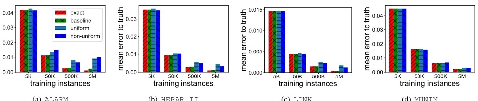
Figure 3 shows the mean relative error to the ground truth for each algorithm. We observe all the algorithms have similar performance when the number of training instances is small, say 5K and 50K. When the number of training instances is large, EXACTMLE has the best accuracy, which is to be expected, since it computes the model parameters based on exact counters. BASELINE has the next best accuracy, closely followed by UNIFORMand NONUNIFORM, that show similar accuracy. Finally, all these algorithms achieve good accuracy results. For instance, after5M examples, the error in estimated event probabilities is always less than one percent, for every algorithm.
. . . 0
WUDLQLQJLQVWDQFHV
UHODWLYHHUURUWRWUXWK
(a) Exact
. . . 0
WUDLQLQJLQVWDQFHV
UHODWLYHHUURUWRWUXWK
(b) Baseline
. . . 0
WUDLQLQJLQVWDQFHV
UHODWLYHHUURUWRWUXWK
(c) Uniform
. . . 0
WUDLQLQJLQVWDQFHV
UHODWLYHHUURUWRWUXWK
[image:10.612.70.553.58.165.2](d) Non-uniform
Fig. 1. Testing error (relative to the ground truth) vs. number of training instances. The dataset isHEPAR II.
. . . 0
WUDLQLQJLQVWDQFHV
UHODWLYHHUURUWRWUXWK
(a) Exact
. . . 0
WUDLQLQJLQVWDQFHV
UHODWLYHHUURUWRWUXWK
(b) Baseline
. . . 0
WUDLQLQJLQVWDQFHV
UHODWLYHHUURUWRWUXWK
(c) Uniform
. . . 0
WUDLQLQJLQVWDQFHV
UHODWLYHHUURUWRWUXWK
[image:10.612.70.554.196.303.2](d) Non-uniform
Fig. 2. Testing error (relative to the ground truth) vs. number of training points. The dataset isLINK.
. . . 0
WUDLQLQJLQVWDQFHV
PHDQHUURUWRWUXWK
H[DFW EDVHOLQH XQLIRUP QRQXQLIRUP
(a)ALARM
. . . 0
WUDLQLQJLQVWDQFHV
PHDQHUURUWRWUXWK
(b)HEPAR II
. . . 0
WUDLQLQJLQVWDQFHV
PHDQHUURUWRWUXWK
(c) LINK
. . . 0
WUDLQLQJLQVWDQFHV
PHDQHUURUWRWUXWK
(d)MUNIN
Fig. 3. Mean testing error (relative to the ground truth) vs. number of training points.
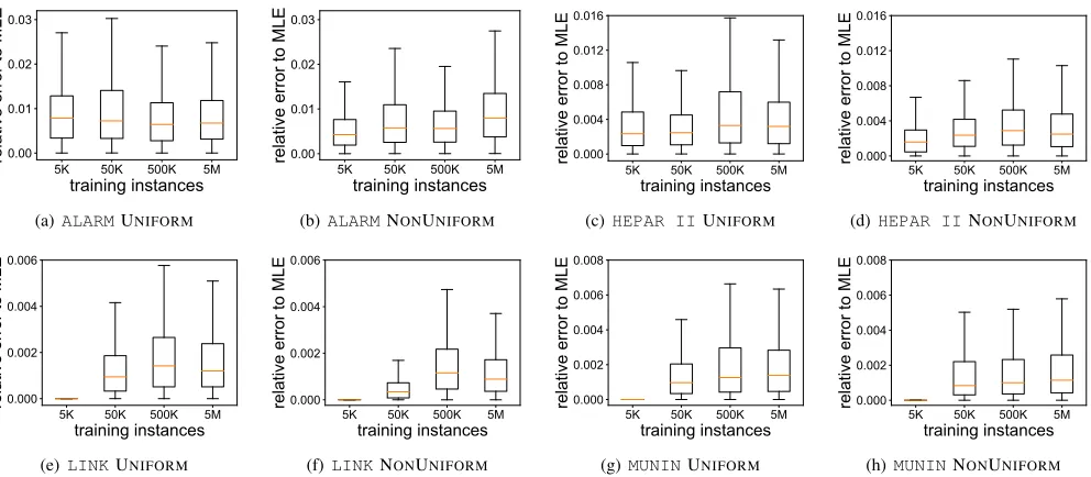
and (2) Approximation error, which is the difference between the model that we are tracking and the model learnt by using exact counters – this error arises due to our desire for efficiency of communication (i.e., trying to send fewer messages for counter maintenance). Our algorithms aim to control the approximation error, and this error is captured by the error relative to exact counter. We note from the plots that the error relative to exact counter remains approximately the same with increasing number of training points, for all three algorithms, BASELINE, UNIFORM, and NONUNIFORM. This is consistent with theoretical predictions since our algorithms only guarantee that these errors are less than a threshold (relative error ), which does not decrease with increasing number of points. The error of NONUNIFORM is usually better than that of UNIFORM, by around 10% on average, varying based on the network used. We conclude that for the “typical” networks evaluated here, we do not observe dramatic differences between UNIFORM and NONUNIFORM. However, since NONUNIFORM is no more difficult to implement that UNIFORM then it is reasonable to prefer it.
Communication Cost vs. Stream Size for different algo-rithms is shown in Figure 6. Note that the y-axis is in loga-rithmic scale. From this graph, we can observe that NONUNI -FORM has the smallest communication cost in general, fol-lowed by UNIFORM. These two have a significantly smaller cost than BASELINE and EXACTMLE. The gap between EXACTMLE and NONUNIFORM increases as more training data arrives. For 5M training points, NONUNIFORM sends approximately 100 times fewer messages than EXACTMLE, while having almost the same accuracy when compared with the ground truth. This also shows that there is a concrete and tangible benefit using the improved analysis in UNIFORMand NONUNIFORM, in reducing the communication cost.
[image:10.612.67.553.334.437.2]. . . 0
WUDLQLQJLQVWDQFHV
UHODWLYHHUURUWR0/(
(a) ALARMUNIFORM
. . . 0
WUDLQLQJLQVWDQFHV
UHODWLYHHUURUWR0/(
(b)ALARMNONUNIFORM
. . . 0
WUDLQLQJLQVWDQFHV
UHODWLYHHUURUWR0/(
(c)HEPAR IIUNIFORM
. . . 0
WUDLQLQJLQVWDQFHV
UHODWLYHHUURUWR0/(
(d)HEPAR IINONUNIFORM
. . . 0
WUDLQLQJLQVWDQFHV
UHODWLYHHUURUWR0/(
(e)LINKUNIFORM
. . . 0
WUDLQLQJLQVWDQFHV
UHODWLYHHUURUWR0/(
(f)LINKNONUNIFORM
. . . 0
WUDLQLQJLQVWDQFHV
UHODWLYHHUURUWR0/(
(g)MUNINUNIFORM
. . . 0
WUDLQLQJLQVWDQFHV
UHODWLYHHUURUWR0/(
[image:11.612.61.557.53.270.2](h)MUNINNONUNIFORM
Fig. 4. Testing error (relative to EXACTMLE) vs. number of training instances. The algorithm is UNIFORMand NONUNIFORM.
. . . 0
WUDLQLQJLQVWDQFHV
PHDQHUURUWR0/(
EDVHOLQH XQLIRUP QRQXQLIRUP
(a)ALARM
. . . 0
WUDLQLQJLQVWDQFHV
PHDQHUURUWR0/(
(b)HEPAR II
. . . 0
WUDLQLQJLQVWDQFHV
PHDQHUURUWR0/(
(c) LINK
. . . 0
WUDLQLQJLQVWDQFHV
PHDQHUURUWR0/(
[image:11.612.57.560.288.713.2](d)MUNIN
Fig. 5. Mean testing error (relative to EXACTMLE) vs. number of training points.
. . . 0
WUDLQLQJLQVWDQFHV
QXPEHURIPHVVDJHV
H[DFW EDVHOLQH XQLIRUP QRQXQLIRUP
(a)ALARM
. . . 0
WUDLQLQJLQVWDQFHV
QXPEHURIPHVVDJHV
(b)HEPAR II
. . . 0
WUDLQLQJLQVWDQFHV
QXPEHURIPHVVDJHV
(c) LINK
. . . 0
WUDLQLQJLQVWDQFHV
QXPEHURIPHVVDJHV
(d)MUNIN
Fig. 6. Communication cost vs. number of training instances.
QXPEHURIVLWHV
UXQWLPHVHF
H[DFW EDVHOLQH
XQLIRUP QRQXQLIRUP
(a)ALARM
QXPEHURIVLWHV
UXQWLPHVHF
(b)HEPAR II
Fig. 7. Training Runtime (on cluster) vs. the number of sites.
QXPEHURIVLWHV
WKURXJKSXWHYHQWVVHF
(a)ALARM
QXPEHURIVLWHV
WKURXJKSXWHYHQWVVHF
(b)HEPAR II
[image:11.612.64.552.306.404.2]
QXPEHURIYDULDEOHV
QXPEHURIPHVVDJHV
H H[DFW EDVHOLQH XQLIRUP QRQXQLIRUP
(a) varies on number of variables
QXPEHURIHGJHV
QXPEHURIPHVVDJHV
H
[image:12.612.59.292.56.168.2](b) varies on number of edges
Fig. 9. Sensitivity test as network scales (extending theLINKnetwork).
and NONUNIFORM algorithms have a significantly shorter runtime, about a half to a third that of EXACTMLE, showing that they can accelerate the Bayesian Network training process. We note the following: (1) the difference between the runtime of NONUNIFORM and EXACTMLE over a network is not as large as the difference in the number of messages, since we are optimizing the number of messages by bundling many updates within a single message. (2) We can expect UNIFORM and NONUNIFORMto perform even better relative to EXACTMLE for streams with more training instances, since the number of messages sent increases only logarithmically for NONUNI -FORM, while it increases linearly for EXACTMLE. We also plot the network throughput, defined as the average number of training points that the system can handle per second in Fig 8. With more sites in the cluster, the network throughput increases, more so for the algorithms built on randomized counters.
Communication vs. Network Size:We test the communica-tion cost under different sizes of networks, from small to large. To build realistic networks of different sizes, we start with the LINK network (which has 724 nodes and 1125 edges), and iteratively remove the sink nodes (outdegree of zero) one after another. This procedure generates eight different networks with {24,124,224,324,424,524,624,724} variables respec-tively. The communication cost for all the algorithms with
500K training instances is shown in Figure 9(a). We observe that the number of messages of the EXACTMLE algorithm increases linearly with the number of variables, as expected from our analysis. For the UNIFORM algorithm, even though the worst case bound on the number of messages isO(n3/2)), we see that the behavior appears closer to linear here. The number of messages sent is never more than a quarter that of the EXACTMLE and BASELINE algorithms. The NONUNI -FORMalgorithm has slightly smaller communication cost than UNIFORM. Our experiments on varying the number of edges in the network shows a similar trend (Figure 9(b)).
Accuracy vs. Approximation Factor: Figure 10 shows the testing error as a function of the parameter , and shows that the testing error increases with an increase in . For small values of , the testing error does not change significantly as changes. This is due to the fact that only controls the “approximation error”, and in cases when the statistical error is large (i.e. small numbers of training instances), the
DSSUR[LPDWLRQIDFWRU
PHDQHUURUWRWUXWK
. .
0 0
(a) Baseline
DSSUR[LPDWLRQIDFWRU
PHDQHUURUWRWUXWK
(b) Non-uniform
Fig. 10. HEPAR IImean error against ground truth vs..
QXPEHURIVLWHV
QXPEHURIPHVVDJHV
[image:12.612.322.552.58.160.2]H EDVHOLQH XQLIRUP QRQXQLIRUP
Fig. 11. Communication cost vs. number of sites, dataset isALARM
approximation error is dwarfed by the statistical error, and the overall error is not sensitive to changes in.
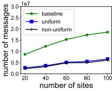
Communication Cost vs. Number of Sites:Figure 11 shows the communication cost as the number of sites is varied, for the ALARMdataset. The plot shows that the number of messages increases sub-linearly with number of sitesk.
Communication Cost of UNIFORMvs. NONUNIFORM:Our results do not yet show a large difference in the communication cost of UNIFORMand NONUNIFORM. The reason is that in the networks that we used, the cardinalities of all random variables were quite similar. In other words, for differenti∈[1, n], the
Jis in Equation 7 and 8 have similar values, and so did the
Kis, which makes the theoretical bounds for UNIFORM and
NONUNIFORMquite similar. To observe the communication efficiency of the non-uniform approximate counter, we gener-ated a semi-synthetic Bayesian networkNEW-ALARMbased on the ALARM network (https://github.com/yuz1988/new-alarm). We keep the structure of the graph, but randomly choose 6
variables in the graph and increased the domain size of these to
20(originally each variable took between2−4distinct values). For this network, the communication cost of NONUNIFORM was about 35 percent smaller than that of UNIFORM.
Classification:Finally, we show results on learning a Bayesian classifier for our data sets. For each testing instance, we first generate the values for all the variables (using the underlying model), then randomly select one variable to predict, given
TABLE II
ERRORRATE FORBAYESIANCLASSIFICATION,50KTRAINING INSTANCES
Dataset EXACTMLE BASELINE UNIFORM NONUNIFORM
ALARM 0.056 0.055 0.053 0.066
HEPAR II 0.191 0.187 0.198 0.212
LINK 0.109 0.110 0.111 0.110
[image:12.612.381.491.187.277.2]TABLE III
COMMUNICATION COST(MESSAGES)TO LEARN ABAYESIAN CLASSIFIER
Dataset EXACTMLE BASELINE UNIFORM NONUNIFORM
ALARM 3.70·106 4.07·105 3.24·105 3.23·105 HEPAR II 7.00·106 1.08·106 7.59·105 7.54·105 LINK 7.24·107 2.98·107 8.22·106 8.06·106 MUNIN 1.04·108 3.44·107 1.13·107 1.13·107
the values of the remaining variables. We compare the true value and predicted value of the select variable and compute the error rate. Prediction error and communication cost for
50K examples and 1000 tests are shown in Tables II and III respectively. We note that even the EXACTMLE algorithm has some prediction error relative to the ground truth, due to the statistical nature of the model. The error of the other algorithms, such as UNIFORM and NONUNIFORM is very close to that of EXACTMLE, but their communication cost is much smaller.
VII. CONCLUSION
We presented new distributed streaming algorithm to esti-mate the parameters of a Bayesian Network in the distributed monitoring model. Compared to approaches that maintain the exact MLE, our algorithms significantly reduce communica-tion, while offering provable guarantees on the estimates of joint probability. Our experiments show that these algorithms indeed reduce communication and provide similar prediction errors as the MLE for estimation and classification tasks.
Directions for future work include: (1) to adapt our analysis when there is a more skewed distribution across different sites, (2) to consider time-decay models which gives higher weight to more recent stream instances, and (3) to learn the underlying graph “live” in an online fashion, as more data arrives.
ACKNOWLEDGEMENT
The work of GC is supported in part by European Research Council grant ERC-2014-CoG 647557 and a Royal Society Wolfson Research Merit Award, and of YZ and ST are supported in part by the National Science Foundation through grants 1527541 and 1725702.
REFERENCES
[1] R. Bekkerman, M. Bilenko, and J. Langford, Scaling Up Machine Learning: Parallel and Distributed Approaches. Cambridge University Press, 2011.
[2] X. Meng, J. Bradley, B. Yavuz, E. Sparks, and et. al., “MLlib: Machine Learning in Apache Spark,”JMLR, vol. 17, no. 1, pp. 1235–1241, 2016. [3] M. A. et al., “Tensorflow: A system for large-scale machine learning,”
inOSDI, 2016, pp. 265–283.
[4] Y. Low, D. Bickson, J. Gonzalez, C. Guestrin, A. Kyrola, and J. M. Hellerstein, “Distributed graphlab: A framework for machine learning and data mining in the cloud,”PVLDB, vol. 5, no. 8, pp. 716–727, Apr. 2012.
[5] Y. Wang and P. M. Djuric, “Sequential bayesian learning in linear networks with random decision making,” inICASSP, 2014, pp. 6404– 6408.
[6] J. Aguilar, J. Torres, and K. Aguilar, “Autonomie decision making based on bayesian networks and ontologies,” inIJCNN, 2016, pp. 3825–3832. [7] P. Xie, J. H. Li, X. Ou, P. Liu, and R. Levy, “Using bayesian networks for cyber security analysis,” inIEEE/IFIP International Conference on Dependable Systems Networks, 2010, pp. 211–220.
[8] D. Oyen, B. Anderson, and C. M. Anderson-Cook, “Bayesian networks with prior knowledge for malware phylogenetics,” in Artificial Intelli-gence for Cyber Security, AAAI Workshop, 2016, pp. 185–192. [9] D. Koller and N. Friedman,Probabilistic Graphical Models: Principles
and Techniques. MIT Press, 2009.
[10] I. Sharfman, A. Schuster, and D. Keren, “A geometric approach to monitoring threshold functions over distributed data streams,” ACM Trans. Database Syst., vol. 32, no. 4, p. 23, 2007.
[11] A. Shukla and Y. Simmhan, “Benchmarking distributed stream pro-cessing platforms for iot applications,” inPerformance Evaluation and Benchmarking. Traditional - Big Data - Interest of Things TPCTC, Revised Selected Papers, 2016, pp. 90–106.
[12] G. Cormode, S. Muthukrishnan, and K. Yi, “Algorithms for distributed functional monitoring,” inSODA, 2008, pp. 21:1–21:20.
[13] M. Balcan, A. Blum, S. Fine, and Y. Mansour, “Distributed learning, communication complexity and privacy,” in PMLR, 2012, pp. 26.1– 26.22.
[14] H. D. III, J. M. Phillips, A. Saha, and S. Venkatasubramanian, “Protocols for learning classifiers on distributed data,” inAISTATS, 2012, pp. 292– 290.
[15] J. Chen, H. Sun, D. P. Woodruff, and Q. Zhang, “Communication-optimal distributed clustering,” inNIPS, 2016, pp. 3720–3728. [16] Y. Zhang, J. C. Duchi, M. I. Jordan, and M. J. Wainwright,
“Information-theoretic lower bounds for distributed statistical estimation with com-munication constraints,” inNIPS, 2013, pp. 2328–2336.
[17] J. M. Phillips, E. Verbin, and Q. Zhang, “Lower bounds for number-in-hand multiparty communication complexity, made easy,” inSODA, 2012, pp. 486–501.
[18] A. McGregor and H. T. Vu, “Evaluating bayesian networks via data streams,” inCOCOON, 2015, pp. 731–743.
[19] B. Kveton, H. Bui, M. Ghavamzadeh, G. Theocharous, S. Muthukrish-nan, and S. Sun, “Graphical model sketch,” inECML PKDD, 2016, pp. 81–97.
[20] G. Cormode, “The continuous distributed monitoring model,”SIGMOD Record, vol. 42, no. 1, pp. 5–14, Mar. 2013.
[21] M. Dilman and D. Raz, “Efficient reactive monitoring,” inINFOCOM, 2001, pp. 1012–1019 vol.2.
[22] R. Keralapura, G. Cormode, and J. Ramamirtham, “Communication-efficient distributed monitoring of thresholded counts,” in SIGMOD, 2006, pp. 289–300.
[23] Z. Huang, K. Yi, and Q. Zhang, “Randomized algorithms for tracking distributed count, frequencies, and ranks,” inPODS, 2012, pp. 295–306. [24] G. Cormode, S. Muthukrishnan, and W. Zhuang, “Conquering the divide: Continuous clustering of distributed data streams,” inICDE, 2007, pp. 1036–1045.
[25] L. Huang, X. Nguyen, M. Garofalakis, J. Hellerstein, A. D. Joseph, M. Jordan, and N. Taft, “Communication-efficient online detection of network-wide anomalies,” inINFOCOM, 2007, pp. 134–142. [26] C. Arackaparambil, J. Brody, and A. Chakrabarti, “Functional
monitor-ing without monotonicity,” inICALP, 2009, pp. 95–106.
[27] Y.-Y. Chung, S. Tirthapura, and D. P. Woodruff, “A simple message-optimal algorithm for random sampling from a distributed stream,”IEEE TKDE, vol. 28, no. 6, pp. 1356–1368, Jun. 2016.
[28] Y. Zhang, S. Tirthapura, and G. Cormode, “Learning graphical models from a distributed stream,”CoRR, vol. abs/1710.02103, 2017. [Online]. Available: http://arxiv.org/abs/1710.02103
[29] M. Scutari, “Bayesian network repository,” http://www.bnlearn.com/ bnrepository/, [Online; accessed May-01-2017].
[30] I. A. Beinlich, H. J. Suermondt, R. M. Chavez, and G. F. Cooper, “The alarm monitoring system: A case study with two probabilistic inference techniques for belief networks,” in Second European Conference on Artificial Intelligence in Medicine, 1989, pp. 247–256.
[31] A. Onisko, “Probabilistic causal models in medicine: Application to diagnosis of liver disorders,” Ph.D. dissertation, Polish Academy of Science, Mar. 2003.
[32] C. S. Jensen and A. Kong, “Blocking gibbs sampling for linkage analysis in large pedigrees with many loops,”The American Journal of Human Genetics, vol. 65, no. 3, pp. 885 – 901, 1999.