Accelerating Kohn–Sham Response Theory using
Density fitting and the Auxiliary-Density-Matrix
Method
Chandan Kumar
1
| Heike Fliegl
1
| Frank Jensen
2
|
Andrew M. Teale
1,3,4
| Simen Reine
1
| Thomas
Kjærgaard
5
1Hylleraas Centre for Quantum Molecular Sciences, Department of Chemistry, University of Oslo, P.O.Box 1033, N-1315 Blindern, Norway
2Department of Chemistry, Aarhus University, Langelandsgade 140, DK-8000 Aarhus C, Denmark
3School of Chemistry, University of Nottingham, University Park, Nottingham NG7 2RD, United Kingdom
4Centre for Advanced Study at the Norwegian Academy of Science and Letters. Drammensveien 78, N-0271 Oslo, Norway 5qLEAP Center for Theoretical Chemistry, Department of Chemistry, Aarhus University, Langelandsgade 140, DK-8000 Aarhus C, Denmark
Correspondence
Chandan Kumar and Simen Reine, Hylleraas Centre for Quantum Molecular Sciences, Department of Chemistry, University of Oslo, P.O.Box 1033, N-1315, Blindern, Norway.
Email: [email protected] [email protected] and
Thomas Kjærgaard, qLEAP Center for Theoretical Chemistry, Department of Chemistry, Aarhus University,
Langelandsgade 140, DK-8000 Aarhus C, Denmark.
Email: [email protected]
Funding information
An extension of the formulation of the atomic-orbital based
response theory of Larsen
et al.
, JCP 113, 8909 (2000) is
pre-sented. This new framework has been implemented in
LSDal-ton and allows for the use of Kohn-Sham density-functional
theory with approximate treatment of the Coulomb and
Exchange contributions to the response equations via the
popular resolution-of-the-identity approximation as well as
the auxiliary-density matrix method (ADMM). We present
benchmark calculations of ground-state energies as well as
the linear and quadratic response properties: vertical
excita-tion energies, polarizabilities and hyperpolarizabilities. The
quality of these approximations in a range of basis sets is
as-sessed against reference calculations in a large aug-pcseg-4
basis. Our results confirm that density fitting of the Coulomb
contribution can be used without hesitation for all the
stud-ied properties. The ADMM treatment of exchange is shown
to yield high accuracy for ground-state and excitation
ener-gies, whereas for polarizabilities and hyperpolarizabilities
the performance gain comes at a cost of accuracy.
Excita-tion energies of a tetrameric model consisting of units of the
P700 special pigment of photosystem I have been studied to
demonstrate the applicability of the code for a large system.
K E Y W O R D S
Kohn-Sham DFT response theory, Density fitting, RI, ADMM
1
|
INTRODUCTION
In molecular electronic-structure theory, an essential step is the evaluation of two-electron integrals over one-electron basis functions. The explicit evaluation of these integrals comes at a high computational cost, and from the dawn of quantum chemistry, approximations have been introduced both to speed up molecular calculations and to reduce memory requirements [1]. Such approximate methods have been widely developed for the calculation of energies and gradients, but less attention has been given to developing these methods for the calculation of molecular properties.
The most widely used approach to approximate the Coulomb and exchange integrals is density fitting [2, 3, 4, 5, 6, 7, 8, 9, 10, 11, 12, 13, 14, 15, 16, 17, 18, 19, 20, 21, 22], also known as the resolution-of-the-identity (RI) approximation. In this approximation products of two one-electron basis functions are expanded in one-center auxiliary functions, and thus, the evaluation of four-center two-electron integrals is replaced by the evaluation of two- and three-center two-electron integrals and the solution of a set of linear equations. RI significantly improves performance with a limited impact on the accuracy and has therefore been applied to Hartree-Fock(HF)/Kohn-Sham(KS) theory, as well as correlated methods [22, 23, 24, 25, 26, 27]. An important alternative approach is the Cholesky-decomposition (CD) technique [28, 29, 30, 31, 32] which to a large extent can be thought of as a special kind of density fitting where the auxiliary basis functions are obtained from the set of products between two one-electron basis functions through Cholesky-decomposition.
Combined withJ-engine techniques [33, 34, 35] RI gives tremendous speed-ups [8, 9] for Coulomb-like
contribu-tions. Although still applicable to exchange [10, 11, 12, 13, 16, 17, 20, 21], the RI methodology does not exhibit the same favorable performance gains as for the Coulomb integrals. Alternative schemes such as the auxiliary-density-matrix method (ADMM) [36, 37] and the chain-of-spheres algorithm (COSX) [38] have therefore been developed specifically for the exchange contribution. In ADMM, the exchange energy is split into two parts. One part consists of the exact HF exchange evaluated in a small auxiliary atomic basis set (from an auxiliary density matrix); the second part is a first-order correction term, evaluated as the difference between the generalized gradient approximation (GGA) exchange in the full and auxiliary basis sets. The auxiliary density matrix can be obtained by means of projection from the full density matrix fulfilling various constraints, as discussed by Guidonet al.[36] and Merlotet al.[37]. The COSX approxima-tion builds on the use of semi-numerical integraapproxima-tion techniques, first introduced by Friesner in the pseudo-spectral method [39, 40, 41] and later refined in the COSX approach by Neeseet al.[38]. In this approach the Coulomb potentials of products of two one-electron basis functions are evaluated analytically on a grid, followed by a numerical integration over the second electron. Reported speed-ups are of up to two orders of magnitude relative to calculations involving explicit exchange-matrix formation [38]. In this work we explore how these techniques may be exploited further in the calculation of molecular properties using response theory.
hyper-polarizability may be evaluated from the linear and quadratic response functions, respectively. In the present work we investigate static (frequency independent) polarizabilities and hyperpolarizabilities. From the poles and residues of the response functions, additional molecular properties can be obtained, including vertical excitation energies to electronically excited states, strength parameters for (multi-photon) transitions to these states, and excited-state properties [42].
Recently, Ringholmet al.[52] presented an approach involving recursion for the open-ended calculation of response properties based on the density matrix-based quasi-energy formulation of the Kohn–Sham density functional response theory using perturbation- and time-dependent basis sets of Thorvaldsenet al.[45]. This approach was extended by Frieseet al.to enable the calculation of single residues of response functions [53, 54]. Very recently, this approach has furthermore been extended to include molecular environment effects by the polarizable embedding model [55].
The RI approximation has been extensively used in connection with CC2 molecular properties [56, 57, 58, 59, 60, 61, 61, 62, 63, 64, 65], but has also been used in connection with the coupled perturbed Kohn–Sham equations[66]. It has also been used in TD-DFT in connection with excitation energies, excited state gradients and frequency-dependent optical rotation calculations [67, 68, 69, 70, 71]. Density fitting can also be applied for the efficient calculation of nuclear magnetic resonance shielding tensors [72, 73]. Ref. 67 and 70 concluded that the auxiliary basis sets developed for ground-state calculations are sufficient for most TD-DFT applications, although in some cases additional diffuse basis functions must be included. Ref. 70 reported that the total computational effort for excited-state optimizations is reduced by at least a factor of 4-6 by the RI-J approximation, with corresponding RI-J errors of 0.01-0.02 eV. The RI-J errors in optimized bond lengths and angles amounted to less then 0.5 pm and 1 degree, respectively. These deviations are usually much smaller than errors due to the incompleteness of the one-particle basis set.
Here we present a method for the computation of approximated response functions within the self-consistent-field (SCF) theories HF and KS density functional theory (DFT) and the extension to include ADMM, density fitting. The current formulation of approximate response theory presented in this work is general and works in principle for all approximations where the approximate Kohn-Sham matrix can be defined as the density matrix derivative of the approximate energy. It allows to easily accommodate future approximate methods that may differ from ADMM or RI in HF/KS response theory.
The approximate response theory formulation introduced in this work is asymptotic linear scaling assuming that sparse matrix algebra is used. However, the focus of the present study is not on the scaling behavior of the approach with system size. Instead we use the new methodology to investigate the impact of the RI and ADMM approximations on the accuracy of linear and quadratic response properties. As examples we consider vertical excitation energies, static polarizabilities and static hyperpolarizabilities for a small benchmark consisting of 11 molecules, and vertical excitation energies for a tetramer P700 model system [74] consisting of 198 atoms. We commence in Section 2 by introducing the theoretical framework for the response calculations. Section 3 shows how this framework can easily accommodate the approximation techniques of the costly Coulomb and exchange integral contributions. Computational details are given in Section 4, and in Section 5 we present results for molecular response properties to assess the relative accuracy of these techniques in practical applications. Finally in Section 6 concluding remarks are drawn and directions for future work are discussed.
2
|
THEORY
follows the response theory method of Larsenet al.[48] with a few modifications emphasizing the role of the Fock/Kohn-Sham matrix, followed by an adaptation to ADMM and RI theories. The derivation assumes that all basis sets employed do not depend on the perturbation. Hence no London [75](gauge including) atomic orbitals nor geometric perturbations are considered in the present work.
2.1
|
Time evolution of the Kohn–Sham system
In Kohn-Sham (KS) density-functional theory (DFT) [76], the time evolution of the spin orbitals, in presence of a time dependent perturbationV(r1,t), is governed by the time-dependent Schrödinger equation [77, 78, 79, 80],
[fKS(r1,t)+V(r1,t)]φj(r1,t)=i
dφj(r1,t)
d t , (1)
where we have introduced the Kohn-Sham operatorfKS(r1,t)=h(r1)+j(r1,t)+vxc(r1,t), which we choose to define
without the perturbationV(r1,t). The Kohn-Sham potentialfKSis defined as the functional derivative of the unperturbed
energy functional
fKS(r1,t)= δE[ρ] δρ(r1) ρ(r1)=ρ(r1,t)
(2)
which depends on the perturbationV(r1,t) through the density
ρ(r,t)=X
µν
χµ∗(r)χν(r)Dνµ, (3)
whereDis the time dependent density matrix in the atomic-orbital (AO) basis andχ(r) denotes the AO basis functions.
In the case of hybrid functionalsfKSmay be supplemented by an orbital dependent term of the form,w ·k(r1,r2,t),
wherewis the weight of orbital dependent exchange andk(r1,r2,t) is the derivative of the exchange energy with respect
to the orbitals, as is used in Hartree–Fock theory.
Eq. (1) may be rewritten as a matrix equation using the expansion in AOsχµ
φi(r1,t)=
X
µ
Cµiχµ(r1), (4)
to obtain [48]
F(D)+V−iS∂ ∂t !
C=SCλ, (5)
with the constituents of the Kohn-Sham matrixF, the time-dependent perturbation matrixVand the overlap matrixS
are given in Eqs. (45-49) of the Appendix. Hereλis a Hermitian Lagrange multiplier matrix. Eq. (5) reduces to the SCF
equation in the perturbation free limit (V= 0) and therefore time-independent limitF(D)C=SCλ.
Multiplying Eq. (5) withCTSfrom the right, subtracting the complex conjugate equation and introducing the density
matrix in the AO basisD=CCTgives [48]
F(D)+V
DS−SD F(D)+V
Using the short hand notationD˙ =∂D∂t for the time derivative of the density matrix. Eq. (6) reduces to the standard
stationary SCF conditionFD0S−SD0F=0in the perturbation free limit, withD0being the optimized AO density matrix for the unperturbed system.
2.2
|
Response Equation
The derivation of the AO-based response equations relies on an exponential parameterization of the density matrix and three expansions. The exponential parameterization of the density matrix, given by
D(X(t))=exp(−X(t)S)Dexp(SX(t)), (7)
with X(t) an anti-hermitian matrix, ensures that the symmetry, trace and idempotency conditions are imposed [81, 82], provided the reference density matrixDalso fulfills these conditions. The transformed density matrixD(X), may be expanded using the the asymmetric Baker-Campbell-Hausdorff (BCH) expansion
D(X)=D0+ [D,X]S+12[[D,X],X] +· · ·, (8)
where the S-commutator is[D,X]S=DSX−XSD. The Kohn-Sham Fock matrixFmay be Taylor expanded around the optimized AO density matrix of the unperturbed state according to
F(D(X))=F(D0)+ ∂D∂F(X) D(X)=D0
(D(X)−D0)
+12 ∂2F ∂D(X)2
D(X)=D0
(D(X)−D0)2+· · ·
=F(D0)+G(D(X)−D0)+1
2T(D(X)−D0,D(X)−D0)+· · ·.
(9)
HereG(M) denotes the first derivative of the KS matrix contracted with a general matrixM
G(M)= ∂F ∂D(X)
D(X)=D0
M
=J(M)+w ·K(M)+Kxc(M), (10)
with the full expressions for the Coulomb matrixJ(M), exchange matrixK(M) and exchange correlation matrixKxc(M) given in Eq. (50) of the Appendix. For the second- (and higher-order) Kohn-Sham matrix derivatives only exchange-correlation contributions remain
T(N,M)= ∂ 2F(D(X))
∂D(X)2 D(X)=D0
(N,M)=Txc(N,M), (11)
withTxc(N,M) given in Eq. (51) of the Appendix.
Finally, the set of parametersX(t) can be expanded in orders of the perturbation
where the zero-order coefficients vanish since the reference state is optimized.
Inserting Eq. (8), Eq. (9) and Eq. (12) into Eq. (6), the parametersX(n)(t) can now be determined by requiring the
resulting equation to be valid to each order of the perturbation. The equation containing the first-order parameters
X(1)(t) is called thelinear response equation, similarly the second-order parametersX(2)(t) are obtained from the quadratic-response equationand so forth.
2.2.1
|
Linear Response Equation
The terms that contribute to the evaluation of theX(1)(t) are
G([D,X(1)]S)DS−SDG([D,X(1)]S) +F(D)[D,X(1)]SS−S[D,X(1)]SF(D) +VDS−SDV=iS[D,X]SS˙ .
(13)
This first-order equation can be solved using the Fourier expansion [48] ofX(1)(t),
X(1)(t)=
∞
−∞exp(
−i ωt)X(1)(ω)d ω (14)
to obtain:
G([D,X(1)(ω)]S)DS−SDG([D,X(1)(ω)]S) +F(D)[D,X(1)(ω)]SS−S[D,X(1)(ω)]SF(D) +VDS−SDV=−ωS[D,X(ω)]SS.
(15)
It can also be written in the shorthand notation [83, 49]
E[2]−ωS[2]
X(ω)=VDS−SDV (16)
with the generalized HessianE[2]defined through the transformation
E[2]X(ω)=−G([D,X(1)(ω)]S)DS+SDG([D,X(1)(ω)]S)
−F[D,X(1)(ω)]SS+S[D,X(1)(ω)]SF, (17)
and the generalized metric matrixS[2]through
S[2]X(ω)=S[D,X(ω)]SS. (18)
Although the frequency is not necessary for the static properties considered in this paper, we include it in the following theory for generality. The excitation energies are identified as the poles of the linear response equation and are therefore solutions to the generalized eigenvalue problem given by
E[2]X
Similarly, for the evaluation ofX(2)(t), the quadratic response equation becomes,
(E[2]−(ω1+ω2)S[2])X(2)(ω1,ω2)= V[D,X(2)(ω1,ω2)]SS−S[D,X(2)(ω1,ω2)]SV
−P12E[3]−(ω1+ω2)S[3]X(1)(ω1)X(1)(ω2).
(20)
The terms contributing to the quadratic response equation are given in Eq. (52) of the Appendix.
2.3
|
Response Functions
Response functions describe the corrections to the expectation value of a Hermitian operatorAˆ, representing an
observable, due to the perturbation
¥˜0` ˆA`˜0¦ = ¥0` ˆA`0¦
+ ∞
−∞¥¥
A;V(ω)¦¦ωexp[(−iω+)t]dω
+12
∞
−∞¥¥
A;V(ω1),V(ω2)¦¦ω1,ω2
exp[(−i(ω1+ω2)+ 2)t]dω1dω2+...
(21)
Using Eq. (8) to parameterize the expectation value
Tr(AD(X))=Tr(AD0)+Tr(A[D,X]S)
+12Tr(A[[D,X],X])+· · ·, (22)
the Fourier expansion ofX, Eq. (14), and collecting orders of the perturbation, one obtains the linear response function
¥¥A;V(ω)¦¦ω=Tr(A[D,X(1)]S), (23)
and the quadratic response function
¥¥A;V(ω1),V(ω2)¦¦ω1,ω2=Tr(A[D,X(2)]S)
+12Tr(A[[D,X(1)(ω1)],X(1)(ω2)]) +12Tr(A[[D,X(1)(ω2)],X(1)(ω1)]).
(24)
3
|
RESPONSE THEORY WITH APPROXIMATE INTEGRALS
energies and excitation eigenvectors can still be determined from Eq. (19).
In this section we derive expressions forGandTfor density fitting and the auxiliary density matrix method (ADMM). This framework is general and can be applied to all approximations where the approximate Kohn-Sham matrix can be defined as the density matrix derivative of the approximate energy. This provides a clear road map for the implementation of response theory using both present and future approximations that accelerate the evaluation of contributions arising from the Coulomb and exchange integrals.
3.1
|
Kohn Sham matrix expansion using density fitting
In density fitting products of two one-electron functions are expanded in auxiliary atom-centered functionsI(r),
according to
`µν¦≈`fµν¦ =X
I
cIµν`I¦, (25)
with indicesµ,ν,ρ,σdenoting the primary AO basis functions, in order to avoid the expensive evaluation of the
four-center two-electron integrals (µν`ρσ). Instead only two- and three-center integrals need to be evaluated, at the expense
of solving a set of linear equations for the coefficientscµνI . The integrals, given in Mulliken notation,
(µν`ρσ)= χµ(r1)χν(r1)r12−1χρ(r2)χσ(r2)dr1dr2, (26)
can be approximated in different ways, for example according to the three term expansion [15]
(µν`ρσ)≈(µν^`ρσ)=(fµν`ρσ)+(µν`ρσf)−(fµν`fρσ), (27)
where the two first terms involve three-center integrals and the last term involves two-center integrals. The different flavors of density fitting arise from the choice of 1) the set of auxiliary functions{I}included in the expansion of Eq. (25), 2) how the fitting coefficientscµνI are obtained and 3) the ansatz for the integral approximation Eq. (27). The set of
functions{I}can range from including only auxiliary functions centered on the two parent atoms [4] ofµandνto the
full set of auxiliary functions on all atoms in the molecule [5, 6]. The fitting coefficients are obtained by minimizing the error∆w
µνof the residual density`δµν¦ = `µν¦−`fµν¦in metricw
∆w
µν= ¥δµν`w`δµν¦ (28)
wherewcan range [12, 14] from the Coulomb operatorr12−1to the Dirac delta function (overlap metric fitting), and
where the minimization can be subjected to charge, dipole or higher-order constraints. The three term ansatz of Eq. (27) is denotedrobust[15] in the sense that it ensures that the errors in the fitted integrals are bilinear with respect to the errors in the two-center fits,
whereas including for instance only the first term has a linear error. We note that when doing the standard (uncon-strained) Coulomb-metric fitting over the full set of auxiliary functions, giving thefittingequation set
X
β
(I`J)cµνJ =(I`µν), (30)
and similarly for`ρσ), the error is bilinear using only the first, second or third (with a positive sign) term of Eq. (27), as it
follows from Eq. (30) that (fµν`ρσ)=(µν`ρσf)=(fµν`ρσf).
When considering external perturbations, one needs to include Lagrangian terms in the integral approximation to ensure that the equations for the fitting coefficients are satisfied with respect to the perturbation. In this paper we only consider perturbations that do not affect the fitted integrals, and the Lagrangian formalism therefore does not need to be considered here. Hence, the application of response theory is straightforwardly achieved by a simple replacement of the exact integrals (µν`ρσ) with the fitted integrals(µν`ρσ^). For the standard density-fitting approximation we simply
replace the exact expressions ofJ(M) andK(M) in Eq. (10), with the approximate expressionsJ˜(M) andK˜(M), given by
˜ J(M)=X
ρσ
^
(µν`ρσ)Mρσ=
X
I
(µν`I)cI,
˜
K(M)=X
ρσ
^
(µσ`ρν)Mρσ=
X
I
X
ρσ
(µσ`I)cρνI Mρσ,
cI ≡
X
ρσ
cIρσMρσ=(I`J)−1
X
ρσ
(J`ρσ)Mρσ,
(31)
to obtain
˜
G(M)= ˜J(M)+w ·K˜(M)+Kxc(M), (32)
where density fitting is used for both Coulomb and exchange. Note, that whereas three-index coefficientscρνI , or
variants thereof [10, 11, 13, 16, 17, 20, 21], are needed for the exchange contribution, only the one-index coefficients
cIare needed for the Coulomb contribution. Additionally, for the Coulomb contribution density fitting can be combined
withJ-engine techniques [8, 9], and as a result greatly outperform the exchange version, thus motivating the search
for alternative approximative approaches for the exchange contribution. In this paper we will consider density fitting for the Coulomb contribution, and investigate the effects of one exchange alternative, the ADMM approach, which is outlined in the next section.
We note finally that approximate Fock/KS matrix construction that requires a decomposition of the density matrix, such as using (local) molecular orbitals[30, 84], cannot straightforwardly be applied in the response framework presented in this paper, as the density matrix dependence changes with the external perturbation.
3.2
|
Kohn Sham matrix expansion using ADMM
The expression for the ADMM energy is based on the following trivial rearrangement of the total exchange energyEK:
where upper-case letters denote quantities evaluated in the primary basis and lower-case letters quantities in the auxiliary basis.Dis the density matrix in the primary atomic-orbital (AO) basis anddis a density matrix obtained by projection ofDto some (smaller) auxiliary electron density. The ADMM exchange energy (EK
admm) is obtained by
replacing the exact-exchange termsEK(D)−Ek(d) in Eq. (33) with exchange functionalsEadmmx [ρ]−Eadmmx [ρadmm]to
give
EadmmK (D)=Ek(d)+Eadmmx [ρ]−Eadmmx [ρadmm] =12 X
α β γδ
dα β(α β`γδ)dγδ+
Ò3x[ρ]dr
−
Ò3x[ρadmm]dr,
(34)
where the Greek lettersα,β,γ,δdenote auxiliary AOs, andρthe electron density
ρ(r)=X
ρσ
χρ(r)χσ(r)Dρσ, (35)
andρadmmthe auxiliary density
ρadmm(r)= X
α β
χα(r)χβ(r)dα β. (36)
Note, that the exchange functional used in the ADMM approximation (denoted with x and admm) may be different from the exchange part of the exchange-correlation functional employed (denoted with xc).
Here we focus on the ADMM2 approximation [36] where the auxiliary density matrixdis obtained through projection, and can be written in terms of the regular AO density matrixDas
d=WDWT, W=s−1Q, (37)
wheresis the AO overlap matrix in the auxiliary basis with elementssα β =χα(r1)χβ(r1)dr1; andQis the mixed auxiliary-primary AO overlap matrix with elementsQα µ =
χα(r1)χµ(r1)dr1. It follows that the ADMM2 exchange
matrix is given by
Kµνadmm(D)=
∂EadmmK ∂Dµν
=Fx,admmµν (D)+WT(k(d)−fx,admm(d))W, (38)
and its resulting derivatives can be expressed as
∂Kadmm(D) ∂D M=K
x,admm(M)
+WT(k(m)−Kx,admm(m))W
∂2Kadmm(D) ∂D∂D MN=T
x,admm(M,N) −WT(Tx,admm(m,n))W
with
m=WMWT, n=WNWT. (40)
Due to the two exchange-functional terms in the ADMM approximation, the exchange contribution will, like the exchange-correlation contribution, have non-vanishing terms for all derivative orders. Here however we limit ourself to quadratic response and thus only up to second order. Using the ADMM2 approximation leads to the following modified expressions for the derivative contributions
Gadmm(M)=J(M)+wKx,admm(M) +wWT(k(m)−Kx,admm(m))W +Kxc(M)
Tadmm(M,N)=wTx,admm(M,N)
−wWT(Tx,admm(m,n))W+Txc(M,N)
(41)
replacing Eq.(10) and (11). Combining density fitting for Coulomb and ADMM for exchange is straightforwardly achieved by substitutingJ(M) with˜J(M) for theGterm of Eq. (41), whereas theTterm remains unchanged. Note that for computational efficiency the ADMM exchange-functional contributions in the regular AO basis can be calculated together with the exchange-correlation contribution simply by augmenting the exchange-correlation functional with the additional ADMM exchange functional terms.
We finally note that developing AO response theory for the flavors of ADMM presented in Ref. [37], ADMMQ, ADMMS and ADMMP, follows the same general principles. However, the expressions become more involved; second-order derivatives require the first-second-order derivative of the scaling factorξand third-order derivatives require the
first-order derivative of both the scaling factorξand the Lagrangian multiplierΛ, in accordance with the2n+ 1and 2n+2rules for variational and Lagrangian parameters, respectively [?]. For the ADMM1 and ADMM3 flavors of Ref. [36]
an AO-based response formulation is not straightforwardly obtained. ADMM1 is MO-based and there is no clear way to differentiate with respect to the AO density-matrix elements. For ADMM3, the same holds when a density-matrix purification method is used.
4
|
COMPUTATIONAL DETAILS
The accuracy of the density fitting and ADMM approximations has been tested on a set of 11 molecules for electronic ground state energies, vertical excitation energies, static polarizabilities and first hyperpolarizabilities. For the vertical excitation energies, the five lowest excitations were considered. The methods under investigation have been run with a local development version of LSDalton [85, 86] on single nodes of a 2.6 GHz Intel E5-2670 cluster, employing OpenMP to utilize the 16 cores on each node.
The test set has been chosen from Ref. [87]. The molecules investigated are acetamide (C2H5ON), acetone (C3H6O), butadiene (C4H6), cyclopropene (C3H4), ethene (C2H4), formaldehyde (CH2O), formamide (CH3ON), furan (C4H4O), imidazole (C3H4N2), propanamide (C3H7ON) and pyrrole (C4H5N). This set of molecules will in the following be denoted as M11.
For each property, the basis set performance of three different types of calculations labeled asfull,df-Jandadmm
Coulomb contribution and LinK [88] for the exchange contribution, i.e. without any approximation (except standard acceleration techniques and integral pre-screening), “df-J” refers to the combination of density fitting for Coulomb and
LinK for exchange, and “admm” to the combination of density fitting for Coulomb and ADMM (ADMM2) for exchange. For the basis set performance, we have chosen the Jensen DFT optimized pcseg-nand aug-pcseg-nbasis sets [89]
as orbital basis, and have investigated the accuracy for cardinal numbersn= 1,2,3against reference aug-pcseg-4
calculations. The prefix “aug” indicates the use of augmented functions. For density fitting the Karlsruhe def2-QZVPP auxiliary basis set of Weigend has been employed[90], for pcseg-nADMM calculations the auxiliary admm-nbasis
sets [91] have been employed, and for the aug-pcseg-nADMM calculations the aug-admm-nbasis sets have been
employed. The admm-nbasis sets have been specifically optimized for the ADMM approximation to be used along with
the pcseg-nfamily of basis sets. The ADMM basis set is developed for elements up to period 3 excluding noble gas
elements. The aug-admm-nbasis sets have been adapted by augmenting the admm-nbasis sets using the augmented
functions from the aug-pcseg-nbasis sets with cardinal numbern−1. The optimized ADMM basis sets are available from a git repository upon request.[92]
In this paper we employ the CAM-B3LYP functional with the specificationsα=0.21,β=0.79 andµ=0.45, rather than
the standard CAM-B3LYP functional parametersα=0.19,β=0.46 andµ=0.33. The main motivation of this choice is to
include full long-range exchange treatment, with the aim to 1) push the errors of the ADMM exchange approximation to its limit, and 2) treat larger systems. For ADMM we have constructed a GGA correction functional, given by Eq. (59) in section 9.4 of the appendix. This GGA correction functional is employed for all calculations involving CAM-B3LYP, with the same functional parameters specifications ofα,βandµas the CAM-B3LYP functional used in the calculation.
For the benchmarks studied here, the molecular size is limited by the time-demanding aug-pcseg-4 reference LinK calculations (the reference calculation on propanamide took roughly 3 weeks to complete). The chosen CAM-B3LYP parameterization is expected to perform well for the properties considered, in particular for polarizabilities and first hyperpolarizabilities, but also for the investigated excitation energies.
As an example application for a larger system, we have calculated the five lowest singlet vertical excitation energies of a tetrameric P700 model, taken from Ref.[74]. The model system is depicted in Figure 11. For these calculations we have employed a hybrid MPI/OpenMP parallelisation scheme, employing 36 nodes each with two 16-core 2.1 GHz Intel Broadwell chips; for a total of 1024 cores.
5
|
RESULTS AND DISCUSSION
Rather than investigating the errors of each method in a given basis set, we have chosen to make a comparison against the basis-set limit. This choice has been taken in order to assess how the methods perform in typical practical calculations. In the following a graphical summary is presented, visualizing normal distributions
f(x)=Nexp*
, −(x−µ)
2 2σ2 +
-(42)
using the mean errorµand the standard deviationσfor each employed approximation, property and basis set. Using
the normalizationNmakes a visual comparison of the differences among methods and basis sets straight forward. For
electronic ground-state energies we have used the normalizationN=log(√1
2σ2π), and for excitation energies, isotropic
polarizabilities, anisotropic polarizabilities and dipole hyperpolarizabilityN= √4 1
2σ2π. For the figures we have chosen to
represent only the “df-J” and “admm” results, since the “full” and “df-J” results are virtually identical, see supplementary
-0.001
0
0.001
0.002
0.003
0.004
0.005
0.006
0.007
0.008
df-J 3
admm 3
df-J 2
admm 2
df-J 1
admm 1
F I G U R E 1 The normal distribution of errors in the molecular ground state energy (in atomic units) with
CAM-B3LYP (α=0.21,β=0.79,µ=0.45)/pcseg-n (n=1, 2, 3) for a set of molecules M11 (see text). Here aug-pcseg-4 results
are taken as the reference.
included maximum absolute errors. These errors do not change the overall picture of the results. As such, we will not discuss maximum absolute errors here, but instead refer the interested reader to the results given in the supplementary information. In the figures, the labels “df-J n” and “admmn” denote a df-Jand admm type calculation, respectively,
employing the pcseg-nbasis sets, and similarly “df-Jaug-n” and “admm aug-n” where the aug-pcseg-nbasis sets are
employed. In the following we use capital letter ADMM for the ADMM approximation and lower case letters admm for the calculations using both df-Jand ADMM.
5.1
|
Electronic ground-state energy
In Figure 1 the normal distributions of the errors in the electronic ground-state energy per electron for pcseg-n, n= 1,2,3, in reference to aug-pcseg-4, are plotted for df-Jand admm calculations. We emphasize again that the full and
the df-Jresults are very similar and we have therefore chosen to present only one of the two in the plots. The results for
all three methods are given in the supplementary information Table S1. Some representative example numbers are presented and discussed in the text below.
While the variance (width) is rather large for both methods when a pcseg-1 basis set is employed a clear improve-ment is seen upon increasing the basis set to pcseg-2 and pcseg-3; the errors are reduced by about one order of magnitude with each cardinal numbern, for all methods. On average all methods investigated overestimate the ground
state energy compared to the aug-pcseg-4 reference, which is to be expected from any variational approach. For example, the mean errors (standard deviations) in a pcseg-2 basis are 458(58), 456(58) and 232(69)µEHfor full, df-J
-0.001
0
0.001 0.002 0.003 0.004 0.005 0.006 0.007 0.008
df-J aug-3
admm aug-3
df-J aug-2
admm aug-2
df-J aug-1
admm aug-1
F I G U R E 2 The normal distribution of errors in the molecular ground state energy (in atomic units) with
CAM-B3LYP (α=0.21,β=0.79,µ=0.45)/aug-pcseg-n (n=1, 2, 3) for a set of molecules M11 (see text). Here aug-pcseg-4
results are taken as the reference.
µEH; all of which are well below1kcal/mol (or 1594µEH). Although the mean error for admm at the pcseg-2 level
is smaller than for the df-Jcalculation by almost a factor two, it is about50% larger in the other two cases, and the
standard deviation for admm is larger in each case.
In Figure 2 the corresponding errors in the electronic ground-state energies are depicted for aug-pcseg-n,n= 1,2,3.
As expected, augmentation leads to some improvement (reducing the errors by10−30%), but does not change the observed trends.
5.2
|
Vertical excitation energies
Figures 3 and 4 show the normal distributions of the absolute errors in the five lowest vertical excitation energies of the M11 benchmark set for df-Jand admm type calculations using pcseg-nand aug-pcseg-nbasis sets, withn= 1,2,3,
respectively. The 55 excitation energies considered here are in the range3.93eV to8.96eV at the reference aug-pcseg-4 full level of theory. The calculations have been run without any point group symmetry, and no attempt has been made to identify the different states. Thus, the order of the excitation energies may vary, in particular for nearly degenerate states, at different basis set and theory levels.
Similar to the trend for the electronic ground-state energies, the excitation energies are overestimated as compared to the aug-pcseg-4 reference. All methods show a systematic improvement with increasing cardinal numbern, and
at each leveln, the full and df-Jtype calculations perform better than admm. Upon augmentation the errors get
0
0.5
1
1.5
2
df-J 3
admm 3
df-J 2
admm 2
df-J 1
admm 1
F I G U R E 3 The normal distribution of errors in the first five excitation energies (in electron volt) with
CAM-B3LYP(α=0.21,β=0.79,µ=0.45)/pcseg-n (n=1, 2, 3) for a set of molecules M11 (see text). Here aug-pcseg-4 results
-0.2
-0.1
0
0.1
0.2
df-J aug-3
admm aug-3
df-J aug-2
admm aug-2
df-J aug-1
admm aug-1
F I G U R E 4 The normal distribution of errors in the first five excitation energies (in electron volt) with
CAM-B3LYP(α=0.21,β=0.79,µ=0.45)/aug-pcseg-n (n=1, 2, 3) for a set of molecules M11 (see text). Here aug-pcseg-4
calculations, respectively. Standard deviations are given in parenthesis. This is already within the range of typical TD-DFT excitation errors, of about 0.1 eV or larger (see for instance Ref. [93]). For aug-pcseg-2 the standard deviations are reduced by another32−47%, and by roughly an order of magnitude further by going to aug-pcseg-3. See supplementary information Table S2 for details.
5.3
|
Static polarizabilities
The normal distribution of the errors in static isotropic polarizabilities at the CAM-B3LYP (α=0.21,β=0.79 andµ=0.45)
level for the M11 benchmark is depicted in Figures 5 and 6, for pcseg-nand aug-pcseg-nwithn= 1,2,3, respectively.
The isotropic polarizabilities are underestimated in all basis sets and at all levels of theory, with a clear improvement for increasing cardinal numbernand upon augmentation. The full numbers are given in Table S3 in the supplementary
information. At the reference aug-pcseg-4 full level of theory, the isotropic polarizabilities of the M11 benchmark range from27.5to55.7a.u. (1a.u. equals (0.529Å)3= 0.148Å3). At the pcseg-1 level the mean errors (standard deviations) are −6.96(2.70),−6.96(2.70) and−7.32(2.88) a.u. for full, df-Jand admm type calculations, respectively, and the errors are
reduced by roughly an order of magnitude, to−0.50(0.20),−0.50(0.20) and−0.84(0.33) a.u., at the pcseg-3 level. Upon augmentation the errors are reduced by one to three orders of magnitude. Already at the aug-pcseg-1 basis the errors are−0.31(0.12),−0.31(0.12) and−1.03(0.45), whereas at aug-pcseg-3 they as low as−3(1),−1(3) and−12(5)ma.u. With
typical DFT errors ranging from0.2to1.0a.u., see for instance Ref. [94], basis sets errors are at an acceptable level from the aug-pcseg-2 level of theory, for all three levels of theory, and remaining basis set errors are essentially removed upon using the aug-pcseg-3 basis set. The admm type calculations have larger errors in all cases, by up to a factor 4 at the aug-pcseg-1 level, and for the aug-pcseg-nbasis the admm errors more or less bisect the values of the full (and df-J)
calculations of cardinal numbersn−1andn.
The error distributions for the static anisotropic polarizabilities are shown in Figures 7 and 8. For the M11 bench-mark the anisotropic polarizabilities range from8.0to47.0a.u. at the reference aug-pcseg-4 full level of theory. Although the mean errors are typically slightly smaller than for the isotropic polarizabilities, the standard deviations are larger; as an example the errors are−0.23(0.35),−0.24(0.36) and−0.38(0.67) a.u. for aug-pcseg-1and−2(3),−8(9) and−21(25)ma.u.
for aug-pcseg-3; see Table S4 in the supplementary information for the full list of mean errors and standard deviations. Similar to the isotropic polarizability, the anisotropic polarizabilities are underestimated using aug-pcseg-nbasis, with
the exception of aug-pcseg-1admm type calculations. For the pcseg-nbasis, the values are instead overestimated. As
for the isotropic polarizabilities the admm aug-pcseg-nerrors fall in between the aug-pcseg-(n−1) and aug-pcseg-n
full errors, although shifted towards the aug-pcseg-(n−1) values, indicating that admm provides a somewhat poorer description of the directional components.
-10
-8
-6
-4
-2
0
df-J 3
admm 3
df-J 2
admm 2
df-J 1
admm 1
F I G U R E 5 The normal distribution of error in the isotropic polarizability (in atomic units) with
CAM-B3LYP(α=0.21,β=0.79,µ=0.45)/pcseg-n (n=1, 2,3) for a set of molecules M11 (see text). Here aug-pcseg-4 results
-1.4
-1.2
-1
-0.8
-0.6
-0.4
-0.2
0
df-J aug-3
admm aug-3
df-J aug-2
admm aug-2
df-J aug-1
admm aug-1
F I G U R E 6 The normal distribution of error in the isotropic polarizability (in atomic units) with
CAM-B3LYP(α=0.21,β=0.79,µ=0.45)/aug-pcseg-n (n=1, 2,3) for a set of molecules M11 (see text). Here aug-pcseg-4
-2
0
2
4
6
8
df-J 3
admm 3
df-J 2
admm 2
df-J 1
admm 1
F I G U R E 7 The normal distribution of error in the anisotropic polarizability (in atomic units) with
CAM-B3LYP(α=0.21,β=0.79,µ=0.45)/pcseg-n (n=1, 2,3) for a set of molecules M11 (see text). Here aug-pcseg-4 results
-0.6
-0.4
-0.2
0
0.2
0.4
0.6
0.8
1
df-J aug-3
admm aug-3
df-J aug-2
admm aug-2
df-J aug-1
admm aug-1
F I G U R E 8 The normal distribution of error in the anisotropic polarizability (in atomic units) with
CAM-B3LYP(α=0.21,β=0.79,µ=0.45)/aug-pcseg-n (n=1, 2,3) for a set of molecules M11 (see text). Here aug-pcseg-4
-30
-20
-10
0
10
20
df-J 3
admm 3
df-J 2
admm 2
df-J 1
admm 1
F I G U R E 9 The normal distribution of error in the BetaParallel (firsthyperpolarizability) (in atomic units) with
CAM-B3LYP(α=0.21,β=0.79,µ=0.45)/pcseg-n (n=1, 2,3) for a set of molecules M11 (see text). Here aug-pcseg-4 results
are taken as the reference.
5.4
|
Static hyperpolarizabilities
To assess how the methods perform for the first hyperpolarizability we have here chosen to study the component of the dipole first hyperpolarizability tensorβ¯along the direction of the permanent molecular dipole momentµ=(µx,µy,µz),
given by [95, 96]
¯ β= 3
5`µ` βxµx+βyµy+βzµz, (43)
with
βξ=
X
ζ=x,y,z
βξζζ, ξ=x,y,z, (44)
whereβξζγare components of the static first hyperpolarizability tensor. Figures 9 and 10 show the normal distribution
of CAM-B3LYP(α=0.21,β=0.79,µ=0.45) errors in the static dipole hyperpolarizabilityβ¯for the M11 benchmark, for
pcseg-nand aug-pcseg-n,n= 1,2,3, calculations, respectively, and more detailed results are reported in Tables S5 of the
supplementary information.
At the reference aug-pcseg-4full calculation the parallel values vary from−41.6to15.3a.u. The standard deviations in the pcseg-nbasis are rather large, and vary from 19.3 a.u. forn= 1to 4.1 a.u. forn= 3, for both df-Jand full type
-4
-3
-2
-1
0
1
2
3
4
df-J aug-3
admm aug-3
df-J aug-2
admm aug-2
df-J aug-1
admm aug-1
F I G U R E 1 0 The normal distribution of error in the BetaParallel (firsthyperpolarizability) (in atomic units) with
CAM-B3LYP(α=0.21,β=0.79,µ=0.45)/aug-pcseg-n (n=1, 2,3) for a set of molecules M11 (see text). Here aug-pcseg-4
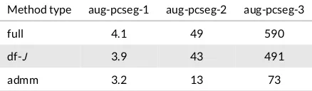
TA B L E 1 Average wall timings in seconds per SCF iteration for the acetone molecule, for ‘full’, ‘df-J’ and ‘admm’ type
calculations (see text for further details).
Method type aug-pcseg-1 aug-pcseg-2 aug-pcseg-3
full 4.1 49 590
df-J 3.9 43 491
admm 3.2 13 73
admm-nresults falls in between the df-J-nand df-J-(n−1) results; for pcseg-nthe admm results are shifted towardn,
and for aug-pcseg-nthe results are less conclusive with the aug-pcseg-2 admm result close to the aug-pcseg-1 full value
and the aug-pcseg-3 admm result slightly shifted towards the aug-pcseg-3 full result.
5.5
|
Performance
In the previous subsections we have presented results for electronic ground-state energies, the first five excitation energies, polarizabilities and first hyperpolarizabilities for the M11 benchmark set. The results show that density fitting for the Coulomb contribution has negligible effects on the results, and that employing ADMM for the exchange can be done in a systematic fashion, albeit at the cost of reduced accuracy. In this section we give our assessment of performance versus accuracy for acetone as an example molecule, to provide an indicative guide for choosing which method to use in practical calculations.
[image:24.485.133.352.82.146.2]Averaged timings per SCF iteration for the three different types of calculation (full, df-Jand admm) are given in
Table 1, for aug-pcseg-ncalculations for the acetone molecule, which is on the median of the 11 molecules with regards
to computational time. The timings for the response part of the calculation are similar, and we refer the interested reader to the supplementary information Table S6 which includes timings for the individual components for both SCF and the response parts of the calculation. In Table 1 full-type calculations are the sum of reg-J, LinK, XC and solver
timings. For the df-Jentry df-Jis used instead of reg-J, and the admm entry is the sum of df-J, ADMM, XC and solver
timings.
The performance gains using density fitting are tremendous when looking at the effect on the Coulomb contribution alone, with speed up factors of 7, 27 and 112 for aug-pcseg-n, with cardinal numbern= 1,2,3respectively. As shown,
this performance boost can be attained at little to no loss in accuracy, and density fitting can thus be applied without hesitation. However, for the hybrid DFT calculations presented here, these speed ups have limited effect on the total timings, with only 5%, 12% and 17% reduction in computational time for the aug-pcseg-nsequence, withn= 1,2,3
respectively. This is because LinK exchange is the main bottleneck for these calculations, amounting for df-Jtype
calculations to 67%, 85% and 95% of the total wall time, forn= 1,2,3.
The motivation to enhance the performance of the exchange contribution should be clear from these results, and the ADMM approximation gives significant speed ups. For the aug-pcseg-nsequence the speed up for the exchange
contribution is a factor of 1.5, 5.8 and 9.7, forn= 1,2,3, respectively. Whilst these speedups are significantly smaller
excitation energies (as done in this paper) are somewhat smaller than for the ground-state energies.
For polarizabilities and hyperpolarizabilities the results are less clear-cut. For the calculation of isotropic polar-izabilities ADMM gives a fairly good description still, whereas for the anisotropic polarpolar-izabilities this is no longer the case. A possible explanation might be the less satisfactory description of transition dipole contributions that do not effect excitation energies but the polarizability and here in particular the anisotropic one where off diagonal elements might have a stronger weight. For hyperpolarizabilities the admm aug-pcseg-3 results reduce the standard deviation of the full aug-pcseg-2 results by a factor 2.9 and the additional computational time is only factor 1.5. Going to the full aug-pcseg-3 the standard deviation is reduced by an additional factor 3.0, now for a factor 8.1 in computational time. Clearly the admm aug-pcseg-3 type calculation is a valid and efficient option. This does not hold for admm aug-pcseg-2 however. Going from aug-pcseg-1 full type calculations reduce the standard deviation by factor 1.2 for an increase in computational time by factor 3.2. Using instead the full aug-pcseg-2 reduces the error by factor 4.5 for a cost of factor 3.7 in calculation time.
In summary, the presented results indicate that density fitting of the Coulomb contribution can be used without hesitation for all properties studied here, although the overall performance gains for hybrid functionals are limited by the efficiency of the exchange contribution. The ADMM exchange approximation can readily be applied for ground-state and excitation energies, whereas for polarizabilities and hyperpolarizabilities the performance gains come at a larger cost in accuracy, making the method of choice less definite.
5.6
|
P700 tetramer model system
Recently, Suomivuoriet. al.[74] published a computational study on the lowest vertical excitation energies of a model system of the special cholorphyll/bacteriochlorphyll pigment center P700 of photosystem I, where the label P700 refers to the absorption peak at 700 nm. The P700 tetramer model is shown in Figure 11. It consists of four chlorin molecules ligated with histidine residues and water. In their study Suomivuoriet. al.[74] used the algebraic diagrammatic construction through second order ADC(2) approach [97, 98], providing highly accurate ab-initio data for a multimeric compound. The P700 tetramer model consists of 198 atoms and serves in the present work as a test system for assessing the accuracy of the different approximative methods applied in our work. It provides also an example for the potential applicability of the LSDalton response module [86] for biologically relevant molecules.
In Table 2 calculated CAM-B3LYP (α=0.21,β=0.79,µ=0.45) results are reported for pcseg-1 and pcseg-2 and
com-pared to those of Ref. [74]. The five lowest vertical transitions have been examined, and the results of augmentation are included at the admm level of theory for aug-pcseg-1 and aug-pcseg-2. The results obtained without any approximation (full) and with density-fitting (df-J) are very similar as compared to the ones of the combined density-fitting and ADMM
approach (admm). An increase of the basis set from pcseg-1 to aug-pcseg-2 leads only to minor changes in the excitation energies, which are slightly decreased by about 0.1 eV or less. The obtained results suggest that augmentation of the basis is not needed for the present system. It appears to be sufficient to use a pcseg-2 quality basis set or even pcseg-1. The calculated CAM-B3LYP (α=0.21,β=0.79,µ=0.45) results agree well with the published ADC(2) reference
values, which have been obtained using the def2-TZVP basis [18]. The def2-TZVP basis is of similar quality as the pcseg-2 basis used in the present work. The experimental value for the lowest transition of the full P700 system lies at 1.77 eV [99, 100, 101, 102]. On ADC(2) level the lowest excitation energy lies at 2.02 eV, while we obtain 1.88 eV for CAM-B3LYP(α=0.21,β=0.79,µ=0.45) with admm/aug-pcseg-2.
For the sake of completeness we also tested different DFT functionals for the present P700 model system. The results for BLYP [103, 104], B3LYP [105, 104], CAM-B3LYP and CAM-B3LYP (α=0.21,β=0.79 andµ=0.45) are
F I G U R E 1 1 P700 -tetramer model system. The coordinates are taken from Ref. [74]
µ=0.33. In this sequence of DFT functionals, the long-range exchange proportion varies from zero to one, starting
from no exchange for BLYP, followed by 0.2 for B3LYP, 0.65 for CAM-B3LYP and full inclusion for CAM-B3LYP (α=0.21, β=0.79 andµ=0.45). Neither the BLYP or the B3LYP functionals describe the P700 tetramer well, and underestimated
the excitation energies by roughly 1.4 eV and 0.8 eV as compared to Ref. [74], respectively. In contrast, the excitation energies obtained with both flavors of the CAM-B3LYP functional perform very well. This can be explained by the improved description of the long-range exchange.
The total computational cost for the pcseg-2 calculations of the five lowest excitation energies using 1024 cores, were 7.4 hours for admm (1.3 h SCF + 6.1 h response), 36.2 hours for df-J(11.5 h SCF + 24.7 h response), and 42.5 hours
for the full calculation (14.2 h SCF + 28.3 h response).
6
|
SUMMARY AND CONCLUSIONS
We have presented an extension to the standard formulation of response theory, which accounts for approximate Fock/Kohn-Sham matrices such as the matrices used in density fitting or the ADMM2 approximation. The development represents a framework to easily introduce the approximate methodologies used in ground-state electronic structure calculations to Hartree-Fock/Kohn-Sham response theory, provided that the Coulomb and exchange matrices can be formulated as derivatives of the approximated Coulomb and Exchange energies.
The option for the combined use of density fitting and ADMM has been implemented and tested in the LSDalton program [86]. An error analysis with respect to different basis sets for full, df-Jand admm type calculations has been
TA B L E 2 Calculated CAM-B3LYP (α=0.21,β=0.79 andµ=0.45) excitation energies in eV for the P700 tetramer
model using the pcseg-1 and pcseg-2 basis sets. Results obtained for the aug-pcseg-1 and aug-pcseg-2 basis sets with admm are given in parenthesis.
state pcseg-1 pcseg-2
full df-J admm full df-J admm Ref. [74]
1 1.95 1.95 1.98 (1.94) 1.89 1.89 1.90 (1.88) 2.02
2 2.00 2.00 2.04(1.93) 1.94 1.94 1.95 (1.93) 2.04
3 2.01 2.01 2.05 (2.01) 1.95 1.95 1.97 (1.94) 2.05
4 2.04 2.04 2.08 (2.04) 1.98 1.98 2.00 (1.98) 2.06
5 2.61 2.61 2.57 (2.56) 2.58 2.58 2.59 (2.58)
TA B L E 3 Calculated excitation energies in eV for the P700 tetramer model using different functionals and admm
approximation. For all calculations the pcseg-2 basis has been used. The CAM-B3LYP results labeled with * are obtained with the specificationsα=0.21,β=0.79 andµ=0.45, rather than the standard CAM-B3LYP functional parameters α=0.19,β=0.46 andµ=0.33.
state BLYP B3LYP CAM-B3LYP CAM-B3LYP* Ref. [74]
1 0.63 1.22 2.06 1.90 2.02
2 0.64 1.23 2.10 1.95 2.04
3 0.68 1.25 2.12 1.97 2.05
4 0.69 1.27 2.14 2.00 2.06
The presented results indicate that density fitting of the Coulomb contribution can be used without hesitation for all properties studied here, although the overall performance gains for hybrid functionals are limited due to the high computational cost of the exchange contribution. The ADMM exchange approximation can be applied to accelerate the evaluation of the exchange contribution, although this entails introducing additional approximations. The ADMM approach was found to work well for ground-state and excitation energies, making it the method of choice for these properties. For polarizabilities and hyperpolarizabilities, although the accuracy with basis set size still improves systematically, the performance gains come at a higher cost in accuracy — making the method of choice less definite.
The lowest five vertical singlet excitation energies for a tetrameric model system of the P700 special pigment [74] of photosystem I have been studied, demonstrating the applicability of the LSDalton response module [86] for a large molecule of biological relevance. Different functionals and basis sets have been tested, and our results indicate that augmentation of the basis is not needed for this system. Satisfactory results can be obtained already on pcseg-1 level, as compared to previously published ADC(2) benchmark data [74], using our combined density-fitting/ADMM approach with the CAM-B3LYP functional.
7
|
SUPPLEMENTARY INFORMATION
See supplementary information for detailed results.
8
|
ACKNOWLEDGMENT
9
|
APPENDIX
9.1
|
Time dependent Schrödinger equation matrix elements
In the time-dependent Schrödinger equation of Eq. (5) the Kohn-Sham matrixFis defined through
Fµν(D)=
δE δDµν =
hµν+Jµν+w Kµν+Kµνxc, (45)
where
hµν=
χµ(r)* ,
−1 2+2I+
X
I
ZI
`r−RI`
+
-χν(r)dr
Jµν(D)=
X
ρσ
(µν`ρσ)Dρσ
Kµν(D)=
X
ρσ
(µσ`ρν)Dρσ
Fµνxc(D)=
χµ(r)vxc(r,t)χν(r)dr,
(46)
with the two-electron integrals in Mulliken form
(µν`ρσ)=
χµ(r1)χν(r1,t)1
r12χρ(r2)χσ(r2)dr1dr2. (47)
The matrix elements of the time-dependent perturbation operator are given by
Vµν=
χµ(r)V(r,t)χν(r)dr, (48)
and the overlap matrix elements are given in the usual form
Sµν=
χµ(r)χν(r)dr. (49)
9.2
|
Kohn-Sham Fock matrix expansion terms
The components of the matrixG(M) in Equation (10) are given by
Jµν(M)=
X
ρσ
(µν`ρσ)Mρσ
Kµν(M)=
X
ρσ
(µσ`ρν)Mρσ
Kµνxc(M)=
χµ(r)
X
ρσ
δvxc
δρ(r,t)χρ(r)χσ(r)Mρσχν(r)drdr
0,
(50)
Fxc(D) to the KS matrix.
In the equation (11), the termTxc(N,M) is given by
Tφξxc(N,M)=X
ρση
MρσNη
χφ∗(r)χξ(r)χρ∗(r0)
χσ(r0)χη∗(r00)χ(r00)
δ2vxc(r) δρ(r)2 drdr
0dr00.
(51)
9.3
|
Quadratic Response Equation
The terms contributing to the linear response equation has been shown in Section 2.2. Here we discuss the terms that contribute to the quadratic response equation.
−
G([D,X(2)(ω1,ω2)]S) +P12G(12[[D,X(1)(ω1)],X(2)(ω2)]) +12P12T([D,X(1)(ω1)]S,[D,X(1)(ω2)]S)
DS
+SDG([D,X(2)(ω1,ω2)]S) +P12G(12[[D,X(1)(ω1)],X(2)(ω2)]) +12P12T([D,X(1)(ω1)]S,[D,X(1)(ω2)]S)
−P12G([D,X(1)(ω1)]S)[D,X(1)(ω2)]SS −1
2P12F(D0)[[D,X(1)(ω1)],X(1)(ω2)]S +P12S[D,X(1)(ω1)]SG([D,X(1)(ω2)]S) +12P12S[[D,X(1)(ω1)],X(1)(ω2)]F(D0) −F[D,X(2)(ω1,ω2)]SS+S[D,X(2)(ω1,ω2)]SF −(ω1+ω2)S[D,X(2)(ω1,ω2)]SS
−1
2(ω1+ω2)P12S[[D,X(1)(ω1)],X(2)(ω2)]S =V[D,X(2)(ω1,ω2)]SS−S[D,X(2)(ω1,ω2)]SV.
(52)
To obtain the expressions above we have used the Fourier expansion ofX(1)(t) (see Eq. (14)) andX(2)(t)
X(2)(t)=
∞
−∞exp(
−i(ω1+ω1)t)X(2)(ω1,ω2)d ω. (53)
andω2. Finally, using the definitions in Eq. (17) and (18) along with
E[3]X(1)(ω1)X(1)(ω2)=
−
G(12[[D,X(1)(ω1)],X(2)(ω2)]) +12T([D,X(1)(ω
1)]S,[D,X(1)(ω2)]S)
DS
+SDG(12[[D,X(1)(ω1)],X(2)(ω2)]) +1
2T([D,X(1)(ω1)]S,[D,X(1)(ω2)]S)
−G([D,X(1)(ω1)]S)[D,X(1)(ω2)]SS −1
2F(D0)[[D,X(1)(ω1)],X(1)(ω2)]S +S[D,X(1)(ω
1)]SG([D,X(1)(ω2)]S) +12S[[D,X(1)(ω
1)],X(1)(ω2)]F(D0)S[3]X(1)(ω1)X(1)(ω2)
(54)
and,
S[3]X(1)(ω1)X(1)(ω2)=12S[[D,X(1)(ω1)],X(2)(ω2)]S (55)
we obtain the well known form of the quadratic response equation of Eq. (20).
9.4
|
The CAM-B3LYP correction functional
The DFT functional CAM-B3LYP [106], is based on a trivial splitting of the Coulomb operator into a short- and a long-range part, according to
1 r12 =
1−α−βerf(µr12)
r12 +
α+βerf(µr12)
r12 , (56)
where the choice of parametersα,βandµspecify the splitting. The error function, erf(µr12), is a smooth function in the range[0−1], starting at zero and approching unity for large distances. The short-range part is evaluated using DFT
ExCAM=(1−α)(ExDirac+ ∆ExB88)−β Exsr, (57)
withExDiracand∆ExB88the Dirac [107] and Becke [103] exchange functionals, andExsrthe short-range exchange
func-tional of Iikuraet al.[108]. The long-range part is evaluated as a range-separated HF exchange contribution
EkCAM=1 2
X
abcd
Dac(ab`
α+βerf(µr12)
r12 `cd)Dbd. (58)
complementary GGA functional
ExCOMP=α(ExDirac+ ∆ExB88)+β Exsr (59)
to approximate the exchange term, Eq. (58), which we employ for the two correction termsEadmmx [ρ]andEadmmx [ρadmm]
in Eq. (33) when using the CAM-B3LYP DFT functional.
R E F E R E N C E S
[1] Simen Reine, Trygve Helgaker, and Roland Lindh. Multi-electron integrals.Wiley Interdisciplinary Reviews: Computational Molecular Science, 2(2):290–303, 2012.
[2] J. L. Whitten. Coulombic potential energy integrals and approximations.J. Chem. Phys., 58:4496–4501, 1973.
[3] J A Jafri and J L Whitten. Electron repulsion integral approximations and error bounds: Molecular applications.J. Chem. Phys., 61:2116–2121, 1974.
[4] E. J. Baerends, D. E. Ellis, and P. Ros. Self-consistent molecular Hartree–Fock–Slater calculations. I. The computational procedure.Chem. Phys., 2:41–51, 1973.
[5] B. I. Dunlap, J. W. D. Connolly, and J. R. Sabin. On some approximations in applications ofXαtheory.J. Chem. Phys., 71: 3396–3402, 1979.
[6] B. I. Dunlap, J. W. D. Connolly, and J. R. Sabin. On first–row diatomic molecules and local density models.J. Chem. Phys., 71:4993–4999, 1979.
[7] O. Vahtras, J. Almlöf, and M. W. Feyereisen. Integral approximations for LCAO-SCF calculations.Chem. Phys. Lett., 213: 514–518, 1993.
[8] Frank Neese. An Improvement of the Resolution of the Identity Approximation for the Formation of the Coulomb Matrix.J. Comput. Chem., 24(14):1740–1747, 2003.
[9] Simen Reine, Andreas Krapp, Maria Francesca Iozzi, Vebjørn Bakken, Trygve Helgaker, Filip Pawłowski, and Pawel Sałek. An efficient density-functional-theory force evaluation for large molecular systems.J. Chem. Phys., 133:044102, 2010.
[10] F Weigend. A fully direct RI-HF algorithm: Implementation, optimised auxiliary basis sets, demonstration of accuracy and efficiency.Phys. Chem. Chem. Phys., 4:4285–4291, 2002.
[11] Robert Polly, Hans-Joachim Werner, Frederick R. Manby, and Peter J. Knowles. Fast Hartree-Fock theory using local density fitting approximations.Mol. Phys., 102:2311–2321, 2004.
[12] Alex Sodt, Joseph E Subotnik, and Martin Head-Gordon. Linear scaling density fitting. J. Chem. Phys., 125:194109, 2006.
[13] A Sodt and M Head-Gordon. Hartree-Fock exchange computed using the atomic resolution of the identity approxima-tion.J. Chem. Phys., 128:104106, 2008.
[14] Simen Reine, Erik Tellgren, Andreas Krapp, Thomas Kjærgaard, Trygve Helgaker, Branislav Jansík, Stinne Høst, and Paweł Sałek. Variational and robust density fitting of four-center two-electron integrals in local metrics.J. Chem. Phys., 129:104101, 2008.
[16] Patrick Merlot, T. Kjærgaard, T. Helgaker, R. Lindh, F. Aquilante, S. Reine, and T. B. Pedersen. Attractive elec-tron–electron interactions within robust local fitting approximations.J. Comput. Chem., 34:1486, 2013.
[17] David S. Hollman, Henry F. Schaefer, and Edward F. Valeev. Semi-exact concentric atomic density fitting: reduced cost and increased accuracy compared to standard density fitting.J. Chem. Phys., 140:064109, 2014.
[18] Florian Weigend and Reinhart Ahlrichs. Balanced basis sets of split valence, triple zeta valence and quadruple zeta valence quality for H to Rn: Design and assessment of accuracy.Phys. Chem. Chem. Phys., 7(18):3297–3305, 2005.
[19] F Weigend. Hartree–Fock exchange fitting basis sets for H to Rn.J. Comp. Chem., 29:167–175, 2008.
[20] Samuel F Manzer, Evgeny Epifanovsky, and Martin Head-Gordon. Efficient Implementation of the Pair Atomic Resolu-tion of the Identity ApproximaResolu-tion for Exact Exchange for Hybrid and Range-Separated Density FuncResolu-tionals.J. Chem. Theory Comput., 15(2):518–527, 2015.
[21] Samuel Manzer, Paul R. Horn, Narbe Mardirossian, and Martin Head-Gordon. Fast, accurate evaluation of exact ex-change: The occ-RI-K algorithm.J. Chem. Phys., 143:024113, 2015.
[22] Frederick R. Manby. Density fitting in second-order linear-r12 Møller-Plesset perturbation theory.J. Chem. Phys., 119 (9):4607–4613, 2003.
[23] M. Feyereisen and G. Fitzgerald. Use of approximate integrals in ab initio theory. An application in MP2 energy calcula-tions.Chem. Phys. Lett., 208:359–363, 1993.
[24] Hans-Joachim Werner, Frederick R. Manby, and Peter J. Knowles. Fast linear scaling second-order Møller-Plesset per-turbation theory (MP2) using local and density fitting approximations.J. Chem. Phys., 118:8149–8160, 2003.
[25] Hans-Joachim Werner and Frederick R. Manby. Explicitly correlated second-order perturbation theory using density fitting and local approximations.J. Chem. Phys., 124:054114, 2006.
[26] Henk Eshuis, Julian Yarkony, and Filipp Furche. Fast computation of molecular random phase approximation correlation energies using resolution of the identity and imaginary frequency integration.J. Chem. Phys., 132:234114, 2010.
[27] Xinguo Ren, Patrick Rinke, Volker Blum, Jürgen Wieferink, Alexandre Tkatchenko, Andrea Sanfilippo, Karsten Reuter, and Matthias Scheffler. Resolution-of-identity approach to Hartree-Fock, hybrid density functionals, RPA, MP2 and GW with numeric atom-centered orbital basis functions.New J. Phys., 14:053020, 2012.
[28] Nelson H. F. Beebe and Jan Linderberg. Simplifications in the generation and transformation of two-electron integrals in molecular calculations.Int. J. Quantum Chem., 12:683–705, 1977.
[29] Henrik Koch, Alfredo Sánchez de Merás, and Thomas Bondo Pedersen. Reduced scaling in electronic structure calcula-tions using Cholesky decomposicalcula-tions.J. Chem. Phys., 118:9481–9484, 2003.
[30] Francesco Aquilante, Thomas Bondo Pedersen, and Roland Lindh. Low-cost evaluation of the exchange fock matrix from cholesky and density fitting representations of the electron repulsion integrals.J. Chem. Phys., 126(19):194106, 2007.
[31] Thomas Bondo Pedersen, Francesco Aquilante, and Roland Lindh. Density fitting with auxiliary basis sets from cholesky decompositions.Theor. Chem. Acc., 124:1–10, 2009.
[32] Francesco Aquilante, Linus Boman, Jonas Boström, Henrik Koch, Roland Lindh, Alfredo Sánchez de Merás, and Thomas Bondo Pedersen. Cholesky Decomposition Techniques in Electronic Structure Theory. In Robert Zalesny, Manthos G. Papadopoulos, Paul G. Mezey, and Jerzy Leszczynski, editors,Linear-Scaling Techniques in Computational Chemistry and Physics. Methods and Applications, volume 13 ofChallenges and Advances in Computational Chemistry and Physics, chapter 13, pages 301–343. Springer, 2011.