Harshness in image classification accuracy assessment
Foody, G. M.
International Journal of Remote Sensing, 29, 3137-3158 (2008)
The manuscript of the above article revised after peer review and submitted to the
journal for publication, follows. Please note that small changes may have been made after submission and the definitive version is that subsequently published as:
Harshness in image classification accuracy assessment
Giles M. Foody School of Geography University of Nottingham
University Park Nottingham
NG7 2RD UK
Abstract
Thematic mapping via a classification analysis is one of the most common applications of
remote sensing. The accuracy of image classifications is, however, often viewed negatively.
Here, it is suggested that the approach to the evaluation of image classification accuracy
typically adopted in remote sensing may often be unfair, commonly being rather harsh and
mis-leading. It is stressed that the widely used target accuracy of 85% can be inappropriate and that
the approach to accuracy assessment adopted commonly in remote sensing is pessimistically
biased. Moreover, the maps produced by other communities, which are often used
unquestioningly, may have a low accuracy if evaluated from the standard perspective adopted
in remote sensing. A greater awareness of the problems encountered in accuracy assessment
may help ensure that perceptions of classification accuracy are realistic and reduce unfair
criticism of thematic maps derived from remote sensing.
1. Introduction
Image classification is one of the most commonly undertaken analyses of remotely sensed data.
In even a cursory sweep of the subject‟s main journals it will be apparent that classification
analyses occur in a significant and often dominant proportion of papers published in many
issues. Despite the importance of classification analysis within the subject, the evaluation of
classifications is, however, a problematic issue.
The main reason for undertaking an image classification is, in effect, to convert the image‟s
information on the spectral response of the Earth‟s surface into a thematic map depicting
classes of interest such as land cover. Given the importance of classification analysis to the
subject area, it is not surprising that considerable research has focused on a wide range of
issues of relevance to its various components. This research has, for example, addressed the
potential of various classification algorithms and the influence of image properties such as the
spatial and spectral resolution as well as of various pre- and post-classification manipulations
on aspects of the analysis. Throughout this research, a major focus has typically been on the
accuracy of the classification.
Classification accuracy has been a focus of attention for a considerable period of time and is a
topic that has developed considerably in recent years (Congalton, 1991, 1994; Congalton and
Green, 1999; Pontius, 2000, 2002; Foody, 2002; Pontius and Cheuk, 2006). Classification
accuracy is the main measure of the quality of thematic maps produced and required by users,
typically to help evaluate the fitness of a map for a particular purpose. The accuracy of image
classification approaches and a suite of issues connected with class discrimination. Although
seemingly a simple concept, classification accuracy is a very difficult variable to assess and is
associated with many problems (Foody, 2002).
The accuracy of image classifications is often perceived as being inadequate for many users
(Townshend, 1992; Wilkinson, 1996; Gallego, 2004). Considerable research has, therefore,
sought to increase the accuracy of thematic mapping through image classification analyses.
However, from a survey of papers published over the 15 year period 1989-2003, Wilkinson
(2005) notes no upward trend in accuracy arising from this effort. Indeed, Wilkinson (2005)
reports no observable trend in classification accuracy over time with a mean accuracy,
expressed as a kappa coefficient of agreement, of ~0.66. It is, therefore, unsurprising that the
accuracy of thematic maps derived from remote sensing is often questioned. Sometimes,
however, this questioning arises from situations in which a map is used for applications other
than those for which it was designed. For example, this problem may occur when a map
developed for specific small cartographic scale applications is used at much larger scales than it
was intended for (Brown et al., 1999). There is also considerable anecdotal evidence of users
questioning the accuracy of maps, often on the basis of very localized assessments (e.g.
arguments like „that pixel is misclassified‟). These and other criticisms of thematic maps
derived from remote sensing may sometimes be unfair. Here, it is suggested that the assessment
and interpretation of classification accuracy in remote sensing may often be made from an
overly harsh perspective. This view is discussed with reference to key widely accepted issues in
accuracy assessment such as the targets used as well as in relation to the assessment of the
2. Accuracy target
The evaluation of the quality of a thematic map derived by an image classification should
ideally be based on a set of criteria defined in advance of its production. As concern is typically
focused on the accuracy of the classification, commonly its overall accuracy, the definition of a
minimum level of accuracy required provides a simple criterion on which to base the
evaluation of classification quality. Thus, classifications are often evaluated in relation to the
magnitude of their estimated accuracy. A target accuracy value should be stated prior to
undertaking the classification, not least because this reduces the potential for very subjective
post-classification evaluations undertaken on a poorly justified ad hoc basis. Although a target
accuracy is often not stated explicitly, one value that has been widely used as a target in
thematic mapping via an image classification is to achieve an accuracy of 85% correct
allocation (e.g. McCormick, 1999; Scepan, 1999; Wulder et al., 2006); it is very rare to see any
other target value specified in the literature. Sometimes this 85% target is qualified further to
indicate that the component classes of the classification should be classified to comparable
levels of accuracy. However, it is against this 85% target that the acceptability of thematic
maps derived from remote sensing is commonly assessed. Indeed, the 85% target is often
viewed explicitly by some as the standard of acceptability for thematic mapping from remotely
sensed imagery (e.g. Wright and Morrice, 1997; Abeyta and Franklin, 1998; Brown et al.,
2000; Treitz and Rogan, 2004).
The 85% target accuracy often seems to be used without question of its suitability and simply
without apparent need for justification or provision of supporting evidence from the literature,
it is essentially seen by many as a universal standard for thematic mapping in remote sensing
(e.g. Fisher and Langford, 1996; Weng, 2002; Rogan et al., 2003; Bektas and Goksel, 2004). It
is not surprising, therefore, that the 85% target has been used in studies spanning a vast range
of applications including the mapping of broad land cover classes at a global scale from 1 km
spatial resolution NOAA AVHRR imagery (Scepan, 1999), mapping of very detailed classes
such as those depicting variations in forest species cover at a very local or large cartographic
scale such as ~1:5,000 from aerial photography (McCormick, 1999) and assessments of change
detection with 30 m spatial resolution Landsat TM imagery (Sader et al., 2001). The studies
reported in these three examples differ greatly in terms of the nature of the classes, the scale of
the study and the characteristics of the remotely sensed data used, yet all adopted the same 85%
accuracy target.
In many cases the origin of this 85% target accuracy can be traced back to the influential work
of Anderson et al. (1976). Indeed this work is often cited explicitly in relation to the
specification of the target accuracy in many projects (e.g. Fisher and Langford, 1996;
Kaminsky et al., 1997; Rogers et al., 1997; Wright and Morrice, 1997; Brown et al., 2000;
Franklin et al., 2001; Lewis and Brown, 2001; Carranza and Hale, 2002; Yang and Lo, 2002;
Weng, 2002; Rogan et al., 2003; Shao et al., 2003; Kerr and Cihlar, 2004; Treitz and Rogan,
2004; Mundia and Aniya, 2005; Yang and Liu, 2005). However, Anderson et al. (1976) do not
discuss the matter in great detail or set out to propose a universally adoptable set of map
evaluation criteria. For example, in the 28 pages of the article there is little discussion of the
article there are actually only two references to the magical 85% figure in the report (both p5),
with the reader directed to an earlier publication by Anderson (1971) for further information.
Anderson (1971) also only briefly discusses the map evaluation criteria. The main focus of both
the Anderson (1971) and Anderson et al. (1976) articles was on the classification schemes that
could be used with remotely sensed data and not on the evaluation of the accuracy of the
derived classifications, although that was clearly an important issue. Both of the articles were
explicitly tentative in their proposals, aware that the sensing technology was rapidly developing
(the articles were written around the time of the launch of the first Earth resources satellite
system, Landsat 1) and that it is unlikely that there is one ideal approach to promote.
Furthermore, both Anderson (1971) and Anderson et al. (1976) were explicit in relation to the
nature of the thematic map under study and have a reason for the 85% figure, which is
specified for a particular application scenario. That scenario was the mapping of broad land
cover classes, such as those at Anderson level I (e.g. urban, agriculture, forest, water etc.), at
small cartographic scales in the range of 1:250,000 to 1:2,500,000. Moreover, the suggestion
made was that
“The minimum level of interpretation accuracy in the identification of land use
and land cover categories from remote sensor data should be at least 85%” and
that the “accuracy interpretation for the several classes be about equal”
(Anderson et al., 1976; p5).
Thus, at the possible risk of misinterpreting the intended meaning, the focus was also not on
This is not the emphasis used in some studies that quote the 85% target accuracy. Additionally,
the basis of the 85% target was because this would be comparable to the accuracy of land cover
maps derived from aerial photograph interpretation undertaken previously in work associated
with the USDA‟s Census of Agriculture. That is, an aim was to emulate the accuracy that could
be achieved for a specific task through the application of conventional approaches such as
aerial photograph interpretation. Additionally, it must be recognised that the minimum
mapping unit for mapping at the specified small cartographic scales is several hundred pixels in
size. If, for example, it is assumed that the smallest unit to be depicted on a thematic map is 2.5
x 2.5 mm in size, the minimum area mapped at a scale of 1:500,000, which is appropriate for
mapping at Anderson level I, is 150 ha (Lillesand and Kiefer, 2000). Thus, in mapping from 80
m spatial resolution Landsat MSS imagery, the type of data considered by Anderson et al.
(1976), the smallest mapped area would comprise at least 234 pixels. Although the component
pixels of the unit mapped might differ in terms of class of allocation the unit would be given a
single label (e.g. dominant class). This is entirely sensible as the map is a generalization of
reality but also highlights the inappropriateness of some pixel based evaluations of image
classifications derived from remote sensing.
The map evaluation criteria put forward by Anderson et al. (1976) were not proposed as being
universally applicable. In the context of satellite remote sensing, the 85% target accuracy was,
essentially, specified by Anderson et al. (1976) for mapping broad land cover classes
(Anderson level I, 9 broad classes) from Landsat 1 sensor data (e.g. MSS with 80 m spatial
resolution in 4 spectral wavebands). The criteria proposed were not, for example, suggested for
satellite sensing systems. It is also questionable whether the 85% target is appropriate for other
small scale mapping applications. For example, the 85% target was used in relation to the
IGBP DISCover global land cover map (Scepan, 1999) yet this map contains 17 classes and
was derived mainly from NOAA AVHRR data with a 1 km spatial resolution (Loveland et al.,
1999). Direct comparison between the IGBP DISCover mapping programme and that
envisaged by Anderson et al. (1976) is difficult (e.g. the generation of the IGBP DISCover map
used multi-temporal data and some ancillary information). However, it is evident that the
Anderson et al. (1976) proposal was made in relation to mapping a small number of classes
from, what may be considered in this context to be, fine spatial resolution multispectral data
with a relatively large minimum mapping unit which is very different to the scenario used in
the production of the IGBP DISCover map, the assessment of which was also based on pixel
level evaluations (Scepan, 1999). Although generalization is difficult, particularly because of
inter-linkages between spatial and categorical scale (Ju et al., 2005) as well as a high degree of
context dependency, classification accuracy commonly, but by no means always, declines with
an increase in the number of classes (e.g. Foody and Embashi, 1995; Joria and Jorgenson,
1996) and/or a coarsening of the spatial resolution of the data (e.g. Irons et al., 1985). An
increase in the detail of the classes is, therefore, generally associated with a reduction in
classification accuracy (e.g Stehman et al., 2003). Note, for example, Vogelmann et al. (2001)
report a 21% decrease in the accuracy for part of the US National Land Cover Data set when
moving from the very general Anderson level I to the more detailed Anderson level II. It,
therefore, seems reasonable to expect that achieving the 85% target would be more of a
challenge for the IGBP DISCover map than the scenario presented by Anderson et al. (1976),
Anderson level I, Landsat MSS data have been used to derive more accurate classifications
than NOAA AVHRR data, especially if the landscape mosaic is heterogeneous (Gervin et al.,
1983). In many contemporary mapping applications, the challenge encountered may also be
more difficult than that presented by Anderson et al. (1976), commonly a result of trying to
map a large number of relatively detailed classes and often at a relatively local, large
cartographic, scale. Consequently, in such applications the use of the 85% target suggested by
Anderson et al. (1976) may be inappropriate as it may be unrealistically high for the
application. Moreover, as mapping scenarios vary enormously in terms of key variables (e.g.
scale and legend detail) and the difficulty of mapping is an interactive function of the classes
(e.g. their number, detail, spatial arrangement etc.) and the remote sensor data used (e.g. spatial
resolution, time of acquisition etc.), there probably is no single accuracy value that could be
adopted universally as a target. Critically, the widely used target of 85% should not
automatically be used as a criterion for the evaluation image classifications (Laba et al., 2002).
It may be that 85% is often a perfectly reasonable target to adopt but it should not simply be
accepted for use without question as for many mapping applications it may be unrealistically
high.
It should be clear, therefore, that the main application scenario of Anderson et al. (1976), from
which the widely used 85% target accuracy appears to have arisen, is very different to many
image classification analyses that have adopted the 85% target. Many studies seek to map
detailed classes at a large cartographic scale (Wilkinson, 2005). Such classes and scales were
explicitly outside the scope of discussion of Anderson et al. (1976) who suggested that
scenario. Yet much of the remote sensing community appears to have latched on to the 85%
target accuracy as some general criterion to apply, irrespective of the specific nature of the
analysis in-hand. Additionally, the community of map users seems to have followed suit and
appear to have adopted the 85% target too. It is unclear why the 85% target has been used so
widely, especially as it may not be realistic. If, for example, the aim is to map a small number
of very spectrally separable classes then the target should perhaps be set at a higher value.
Alternatively, and perhaps more commonly, if there are many classes that are only subtly
different it seems reasonable to ask if the target accuracy is too high and unachievable. To be of
value, a target should really be specified for the particular application in-hand and be realistic.
Instead of seeking a single universally applicable target value, it would often seem to be more
appropriate to set a target for the specific application in-hand; for general purpose maps,
producer‟s can provide accuracy information to enable user‟s to determine the data set‟s
suitability for their specific needs. The target value to adopt may be expected to vary as a
function of variables such as the nature of the remotely sensed data set used (e.g. spatial and
spectral resolution), the classes defined (e.g. number and detail of classes) and user needs (e.g.
tolerance to error and impacts of variation in error severity). There are, therefore, no universally
defined accuracy standards for thematic mapping from remote sensing (e.g. Loveland et al.,
1999; Kerr and Cihlar, 2004). However, since accuracy relates fundamentally to the fitness for
purpose, it should be possible to define the level of accuracy required for the application
in-hand. This accuracy value represents the minimum required for the application, it may be less
than the accuracy level wanted by users but is sufficient to meet their needs. The required
about tree species diversity and co-existence, Atkinson et al. (2007) required maps showing the
spatial distribution of ash and sycamore trees in a mixed woodland. Although tree species may
be considered to form very specific classes, more detailed than those at Anderson levels I and
II, trees can sometimes be identified to species level with a high accuracy from remotely sensed
data. However, a high accuracy may not actually be required. Indeed, for the seemingly
complex application of mapping detailed classes, each representing an individual tree species,
such that the degree of species aggregation in space can be determined required an image
classification in which omission errors of 50% and commission errors of 5% for the species of
interest could be tolerated (Atkinson et al., 2007). In such circumstances, especially as there
was a large number of other species in the woodland, the overall accuracy of an image
classification that provided the necessary information could be very low, perhaps in the order
of ~10%. Clearly one would normally want and should strive for a higher accuracy but a
classification of apparently low accuracy can still yield the information required for the
application in-hand.
One issue on which the remote sensing community could, however, adopt a harsher approach is
in deciding whether a thematic map produced by an image classification satisfies the target
specified. Commonly, the basis of assessing the acceptability of a map is to calculate a measure
of the map‟s accuracy and compare the derived value directly against the target value (e.g.
Hayes and Sader, 2001). The map is typically judged to be sufficiently accurate if the
calculated accuracy value equals or exceeds the target. However, the accuracy statement
instances it would be more appropriate to fit confidence limits to the estimate and consider
these when evaluating the map and deciding if the target accuracy has been achieved.
Although the estimation of confidence limits is relatively simple and the literature encourages
the community to use them (Thomas and Allcock, 1984; Morisette and Khorram, 1998; Mas,
2004) they are rarely defined and provided. In many applications, the accuracy statement for an
image classification should, however, really take the form of the estimated value ± the half
width of the confidence interval at some specified level of statistical confidence. Assuming
that the analysis is based on a sufficiently large sample of data acquired by simple random
sampling and that the data are normally distributed, the half width of the confidence interval
may be derived from
1 ) 1 ( n p p
t where p is the proportion of correctly allocated cases, n the
number of cases used to assess classification accuracy and the value of t is derived from the
t-distribution at the desired level of confidence (for large sample sizes the value of t approaches
that for the appropriate z-score).
The fitting of confidence limits around the estimate of classification accuracy may have a
marked impact on the evaluation of a classification. Sometimes the estimated accuracy of a
classification may exceed the 85% target value but the confidence limits may suggest that it
would be unwise to assume that this means the classification has achieved the target level
desired. However, a classification with an estimated accuracy that barely exceeds the target
value specified is often viewed as being of acceptable quality (e.g. Hayes and Sader, 2001). For
derived from a classification as being satisfactory as its estimated accuracy, 89.5%, exceeded
the commonly stated target of 85%. Fitting, the albeit wide, confidence limits at the 98% level
to the accuracy estimate, it may be stated that with 0.98 probability that the map‟s accuracy lies
within the range 84.7 - 94.2%. The lower limit of this confidence interval lies below the 85%
target and so, at this level of assessment, the map might not be viewed as being sufficiently
accurate. At the more widely used 95% level of confidence, the map just passes the threshold
as its accuracy may be expressed as 89.5 ± 4.00%, with the lower limit on the confidence
interval just over the target accuracy at 85.5%. Note, however, that with just 1 more
misclassification in the testing set used to estimate accuracy the resulting classification would
have had an accuracy of 89.0 ± 4.08% at the 95% level of confidence, failing to achieve the
target as the lower confidence limit again lies below 85%. The casual comparison of the
accuracy estimate directly against the target may, therefore, give an inappropriate basis for
evaluating a classification. The confidence limits fitted around the estimated value provide
important information that should influence the evaluation of the accuracy of the classification
and its suitability for later application. The confidence limits are also useful in the comparison
of classification accuracy statements. In such applications it is, however, also necessary to
recognise the nature of the testing set used in the estimation of accuracy, particularly if the
same testing set is used in the evaluation of different classifications (Foody, 2004). Critically,
however, the remote sensing community should be encouraged to fit confidence limits to
classification accuracy statements and promote their use in evaluating the classification‟s
fitness for its intended application.
The most widely used approaches for image classification accuracy assessment are site-specific
methods based on the analysis of the entries in a confusion or error matrix (Congalton and
Green, 1999; Foody, 2002). In principal, this matrix provides a simple summary of
classification accuracy and highlights the two types of thematic error that may occur, omission
and commission. This not only summarises the accuracy of the classification but may also
convey useful information to enhance analyses based on the classification (e.g. Prisley and
Smith, 1987; Fang et al., 2006). In reality, however, the use of the confusion matrix and
interpretation of the accuracy measures derived from it can be distinctly non-trivial activities.
For example, the meaning of basic summary measures of accuracy such as the proportion of
correctly allocated cases, the most widely used index of classification accuracy, is a function of
the sample design used in acquiring the testing set (Stehman, 1995). Thus, the estimates of
classification accuracy derived from confusion matrices constructed from testing sets drawn by
simple random and stratified random sampling from the same map, without any allowance for
the difference in the sample design, may differ substantially if the classes vary in abundance
and spectral separability. Additionally, the use of the confusion matrix is based implicitly on
the assumption that the pixels are pure and the ground data set is perfectly co-located with the
image classification. Both of these assumptions are rarely satisfied. The proportion of mixed
pixels in an image is a function of the spatial resolution of the imagery and the land cover
mosaic but is often very large. These pixels cannot be accommodated directly in the basic
confusion matrix resulting in error. Similarly, much error depicted in a confusion matrix is
associated with mis-location of data points in the thematic map and in the ground or reference
data. Moreover, there is also a tendency to treat the ground data set as being error-free. The
1996; Khorram, 1999; Mas, 2004) and the direct comparability of the data sets may be limited
by the use of different ontologies such that the two data sets may appear to have the same set of
classes but their meaning may differ (Comber et al., 2005). There are other major sources of
error to be considered. For example, geometric pre-processing operations can introduce very
large errors in the representation of classes and this can greatly impact on studies such as
change detection (Rocchini et al., 2004). Despite the various problems with the confusion
matrix, all of the disagreements between class labels in the thematic map derived from
remotely sensed data and the ground data are typically interpreted, unfairly, as errors in the
classification used to produce the thematic map (Fitzgerald and Lees, 1994; Foody, 2002). This
perspective provides a pessimistically biased starting point for the quantification of
classification accuracy.
A key concern in the evaluation of a classification is that the confusion matrix, which is
fundamental to contemporary accuracy assessment (Congalton, 1994; Congalton and Green,
1999), is associated with considerable uncertainty and error, including non-thematic error. The
problems associated with the use of the confusion matrix are often ignored in accuracy
assessment yet will generally act to reduce the magnitude of the estimate of classification
accuracy. Thus, not only may the target accuracy be unrealistically high, the approach to assess
accuracy may act to give an unfairly negative view of the quality of the thematic map.
However, this site-specific and typically pixel-based approach to accuracy assessment is
commonly used, even if the various sources of error and uncertainty such as those arising from
mis-registration are recognised (e.g. Zhu et al., 2000). The standard approach to accuracy
rather than rigidly adopt the site-specific comparison the accuracy assessment could perhaps be
based on the modal class in, say, a 3x3 pixel window (Vogelmann et al., 2001; Stehman et al.,
2003) or use made of modified accuracy measures that attempt to provide a degree of tolerance
for mis-location (Hagen, 2003). It is important, however, to avoid the potential to optimistically
bias the accuracy assessment. Similarly, it is important to be aware that some promoted
manipulations of the confusion matrix, such as normalization, can be undesirable (Foody,
2002; Stehman, 2004). Normalizing the matix has the effect of equalizing what may actually be
very different user‟s and producer‟s accuracies and the normalized matrix needs to be used and
interpreted with care.
The problems in constructing a meaningful confusion matrix, sometimes the one of the hardest
parts of accuracy assessment (Smits et al., 1999), and interpreting its contents are often
compounded by the use of inappropriate measures to quantify classification accuracy. There
are, for example, many calls for the remote sensing community to adopt measures such as the
kappa coefficient of agreement in the assessment of classification accuracy (Congalton et al.,
1983; Congalton and Green, 1999; Smits et al., 1999; Wilkinson, 2005). The arguments made
for the adoption of the kappa coefficient are typically based on statements such as its
calculation corrects for chance agreement and utilizes the entire confusion matrix as well as
that a variance term can be calculated for it which facilitates statistical comparisons and
because scales exist to aid interpretation (e.g. Congalton et al., 1983; Monserud and Leemans,
1992; Janssen and van der Wel, 1994; Smits et al., 1999; Wheeler and Alan, 2002). The use of
the kappa coefficient for accuracy assessment has, however, often been questioned (Stehman,
kappa coefficient as a measure of classification accuracy can be readily criticised. Some of the
arguments made for the adoption of the kappa coefficient are incorrect. For example, the kappa
coefficient is not calculated from the entire matrix but on the basis of its main diagonal and
marginals (Stehman, 1997; Nishii and Tanaka, 1999). Some of the arguments for the adoption
of the kappa coefficient fail to recognise that they apply equally to other measures of accuracy.
For example, a variance term can be derived for many other measures of accuracy that are
widely used, including standard statements based on the percentage of correctly allocated cases,
and be used in evaluating the statistical significance of differences in classification accuracy
(Foody, 2004). In addition, widely used scales to interpret the kappa coefficient are problematic
and arbitrary (Manel et al., 2001; Di Eugenio and Glass, 2004). Most critically of all, the
allowance for chance agreement, probably the most widely cited reason for the adoption of the
kappa coefficient as a measure of classification accuracy, has been criticised in several ways. In
particular, it is evident that the degree of chance agreement may be overestimated, leading to an
underestimation of classification accuracy (Foody, 1992), and, more fundamentally, that chance
correction is completely unnecessary (Turk, 2002). The fact that some of the class allocations
in the classification are correct by chance and not by design is a lucky break or windfall gain, it
is not necessarily something the users or producers of thematic maps should worry about.
Essentially, if the aim is to state the accuracy of a thematic map derived from an image
classification then the source of error is unimportant. What is required in such circumstances is
an index of map accuracy and not of the map producing technology. One such index that may
commonly be appropriate is the percentage of correctly allocated cases. If, however, the aim is
approach for that application might be to calculate a measure of diagnostic ability (e.g. Turk,
1979) rather than classification accuracy.
Despite its limitations, the use of the kappa coefficient and related approaches over the last ~20
years has encouraged an increasingly rigorous and quantitative evaluation of classification
accuracy which should be regarded as a useful, if somewhat incorrect, step in the direction
towards an appropriate evaluation method. The key concern here, however, is that the use of
measures such as the kappa coefficient may have the effect of suggesting on naïve inspection
that classification accuracy is lower than it really is. In particular, the removal of chance
agreement compounds the common problem of adopting a pessimistically biased perspective in
accuracy assessment by adding a pessimistic bias to the quantification of accuracy.
4. Comparison with other mapping communities
While the remote sensing community is gradually moving toward a position in which an
accuracy assessment is seen as an essential component of a mapping exercise (Cihlar, 2000;
Strahler et al., 2006) this is not always the situation with other mapping communities. The
remote sensing community may be being rather harsh on itself by setting high standards and
using techniques that commonly act to reduce the apparent accuracy of a classification while
the producers of other maps use very different approaches and criteria. Typically other mapping
bodies, while concerned about map quality, provide little or no information on map accuracy or
have relatively loosely defined and tolerant criteria of acceptability. This is not a criticism of
however, that the remote sensing community may be harsher in the evaluation of its products
than other mapping communities are of theirs. The user community also appear harsher in their
assessments of thematic maps produced by remote sensing than other widely used maps. To
illustrate this variation in the harshness of evaluations, the approaches adopted by parts of three
other communities, those concerned with geological, soil and topographic mapping, will be
briefly discussed.
4.1 Geological maps
The British Geological Survey claims that its maps are amongst the most accurate geological
maps in the world (Smith, 2004). This may well be true but the maps are not accompanied by
accuracy statements of the type commonly provided with thematic maps derived from remote
sensing. Indeed the accuracy information provided generally available relate predominantly to
the spatial and cartographic components of the map rather than the thematic, geological,
information contained. There may, however, be an increase in attention to the accuracy of the
geological information content in the future.
A geological map is simply an interpretation of the geology, a difficult and subjective task as
much of the geology is, of course, concealed. Critically, however, the accuracy statement
generally provided with geological map data explicitly does not address the quality of the
geological linework or data in general as much of this is a matter of interpretation. As all
geological units are either represented by a line or contained within a set of lines, the linework
of the map is of fundamental importance yet its meaning is very uncertain. Plotted boundaries
an actual boundary may occur. Moreover, the linework does not distinguish between the
different types of boundary that may occur and the vast majority of the boundaries plotted are
inferred with many being little more than best guesses. The geological community is no doubt
aware of the general nature of the maps, including their limitations, and appears to simply
factor this information into its work when using them. Such maps are, however, clearly likely
to contain error when viewed from the overly harsh site-specific approach to accuracy
assessment used in remote sensing. Given that the boundaries depicted on a geological map are
clearly a simplified generalisation, rigidly accepting them and using testing sites in their
vicinity in an assessment of accuracy is likely to be a major source of error. Indeed
misclassification in boundary regions has commonly been noted as a major source of error in
thematic maps derived from classifications of remotely sensed data. For example, the accuracy
of a land cover map of Great Britain increased by ~25% to ~71% when boundary regions were
excluded from the evaluation (Fuller et al., 1994).
4.2 Soil maps
As with geological mapping, there has been a long history of mapping soils and there is
considerable dependence on interpretation. Generally, soil maps show the spatial distribution of
soil type classes over a region. These classes are often rather uncertainly defined. For example,
in the UK a soil map may show the dominant soil series (Curtis et al., 1976). Thus, a mapped
polygon might be dominated by one class but some of its area may comprise a number of other
soil classes. Moreover, the amount of inclusion is not always evident. Some polygons may
contain substantial mixtures of soil types and simply be represented in the map as mixtures.
boundaries are located on the basis of surveyor‟s judgements. In the USDA‟s soil maps, up to
25% (occasionally >50%) of a mapped polygon may actually be of a type other than that
labelled (Soil Survey Division Staff, 1993). Clearly a large proportion of the total mapped area
may, therefore, be mis-labeled. Thus, as a simplistic example, a soil map deemed to be
completely accurate (100% correct) in which every mapped unit had a 25% inclusion rate
would have an accuracy of 75% if evaluated from the perspective adopted in remote sensing.
Additionally, a further concern is that the degree of correspondence between the soil map
description and field observation may be variable and this has important implications to using
the soil data for modelling in a GIS (Drohan et al., 2003). As with geological maps, relatively
little information on thematic accuracy is provided and there is considerable potential for error
when viewed from the harsh site-specific perspective adopted in remote sensing. The
evaluation of soil map accuracy is, however, seen as a research topic and, as recognised in
other mapping communities (Maling, 1989), one that could benefit from reference to accuracy
assessment methods used in remote sensing (McBratney et al., 2003).
4.3 Topographic maps
Topographic maps are perhaps the most widely used form of mapped information and the main
alternative form of map to thematic maps. The quality of such maps is typically evaluated in
terms of a range of variables such as positional accuracy, completeness and attribute accuracy
(Maling, 1989; Thapa and Bossler, 1992). A major concern with topographic mapping is
typically to correctly represent the relief and key physical features of the landscape. Accuracy
statements, therefore, typically focus on the vertical and horizontal errors present in the data
of map accuracy standards. For example, in relation to positional accuracy, topographic maps
are normally considered accurate if the horizontal and vertical errors contained are below some
specified threshold levels. Although positional and thematic accuracy are different variables
they are the fundamental properties of topographic and thematic maps respectively. The
differences between these two types of accuracy make direct comparison of the approaches to
evaluate accuracy difficult. However, in relation to the evaluation of the accuracy of a map, it
seems likely that the assessment of a topographic map is less harsh than that applied to
thematic maps derived from remote sensing. This may be illustrated with an example in which
errors in a topographic data set were treated as if thematic errors in a thematic map derived
from a classification analysis.
4.3.1 Topographic map accuracy
A simple experiment may be used to provide a rough guide to the accuracy of topographic
maps when assessed from the standard accuracy assessment perspective used in remote
sensing. A key issue in topographic mapping is the accurate representation of height. Here, the
accuracy of height information in a topographic data set that satisfied conventional topographic
mapping standards was assessed using the site-specific accuracy assessment approach widely
adopted in remote sensing.
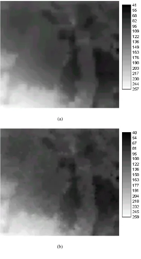
A small extract of a digital elevation model (DEM) for a region of hilly terrain in north Wales,
UK, was acquired. The DEM provided information on location (X and Y) and terrain height
(Z) for the region with a spatial resolution of 25 m. Within this region, the range in terrain
used to generate a finer spatial resolution surface of the region. For this, the raster DEM data
was converted to vector (point) format and a new DEM with a spatial resolution of 1 m derived
via a basic interpolation algorithm. This provided a fine spatial resolution terrain surface for the
region that was assumed here to be the actual (error-free) terrain surface (Figure 1a).
A further surface that could be taken to be the mapped or modelled representation of the actual
situation was produced (Figure 1b). This was designed to satisfy the standard type of horizontal
and vertical tolerances allowed in topographic mapping (Maling, 1989). Here, a widely used
US standard for mapping at 1:24,000 scale was adopted. As the mapped representation was
designed to satisfy the map standard it would be considered an accurate representation of the
actual surface.
The mapped surface was derived by adding distortions to the actual surface. With the widely
used US map accuracy standards for 1:24,000 scale mapping, a horizontal accuracy such that a
sample of 90% of points lie within 40 feet (~12.2 m) of their actual location and a vertical
accuracy such that 90% of points lie within a half-width of the contour interval is required for
the map to be considered accurate (Maling, 1989). Using the vector file derived from the actual
surface, horizontal errors that satisfied the horizontal map standards were introduced into the
data set. This was achieved by adding random values with a uniform distribution within the
range -7 to +7m to X and to Y for 90% of the points in the actual surface data set. The
remaining data were divided into two equally sized data sets and given larger errors. For these
data sets, random values with a uniform distribution between -8 to -14 m and 8 to 14 m were
coordinates of the data set their effect on the horizontal accuracy was assessed. This revealed
that 90% of the points lay within 11.7 m of their actual location, satisfying the requirement for
an accurate map.
A similar approach was taken to distort the actual height (Z) data. Assuming that the mapped
data would have a 10 m contour interval, typical of many maps, distortions were added to the
actual Z values. Specifically, for 90% of the points selected at random from the data set,
random values with a uniform distribution from -5 to +5 m were added to the data. The
remaining data were divided into two equally sized data sets and given larger distortions. Here,
the values applied to these data sets were in the range -6 to -10 m and 6 to 10 m. Given that the
mapped representation had a contour interval of 10 m, the data set derived in this manner also
satisfied the vertical mapping standard for a map to be considered accurate.
The derived data set used to form the mapped representation, therefore, satisfied both the
horizontal and vertical mapping standard specified. Consequently, the mapped representation
would be considered accurate. Indeed the mapped and actual representations were very highly
correlated, r=0.997 (significant at the 99.9% level), and the RMSE was estimated to be 5.8 m,
indicating a quality of broadly similar magnitude to digital elevation models reported in the
literature (e.g. Bolstad and Stowe, 1994; Giles and Franklin, 1996).
The accuracy of the map was, however, also assessed from the standard remote sensing
perspective. For this, height information in the actual and mapped representations were
sample of 1678 locations, the height value depicted in the actual and mapped representations
was extracted from the data set. Cross tabulating the height class in the actual and mapped
representations yielded a confusion matrix from which basic measures of classification
accuracy could be derived. From this confusion matrix, it was estimated that the accuracy of
the height information depicted in the mapped representation was 65.5%. Thus the mapped
representation, which satisfied the basic map accuracy standards, would appear to be of
relatively low accuracy when evaluated from the harsh perspective used in remote sensing. It
should be noted, however, that much of the error was, as expected, associated with
neighbouring classes. Since the height classes defined lie on an ordered scale, the severity of
misclassification error varies as a function of the dissimilarity of the classes and this is not
accommodated in the basic approach to accuracy assessment used in remote sensing which
treats all errors as being of equal magnitude. Thus, the derived estimate of accuracy could be
considered to under-represent the map‟s actual quality. It is also important to note, however,
that many classifications of remotely sensed data include related or ordered classes but are
evaluated in the standard way with all errors weighted equally (e.g. Joria and Jorgenson, 1996;
Rogan et al., 2003). For example, 5 of the 17 classes depicted in the IGBP DISCover map are
of forest and for some users mis-allocations amongst these classes may be of no consequence.
Indeed for some user‟s the accuracy of the IGBP DISCover map rises from a stated accuracy of
~78% to ~90% after the aggregation of appropriate classes (DeFries and Los, 1999).
Clearly, the scenario presented above is limited. It is not meant to be taken as a rigorous and
thorough example but merely one that indicates the general trend using reasonable values for
representation that was more erroneous (e.g. there is no upper limit to the error magnitude for
the 10% of cases that can lie beyond the target level specified). Similarly, the analysis could as
easily be adjusted to show less error (e.g. use of a test site with little variation in height). The
key concern is that, using reasonable error values on a data set of moderate relief, the accuracy
of the topographic information was low when viewed from the perspective often used in
remote sensing. To further illustrate this, it would be necessary for the class width to be
increased three times, to 30 m, for the accuracy to rise above the 85% accuracy standard widely
promoted in remote sensing. Specifically, with a 30 m class width the accuracy was 86.3 ± 1.6
% at the 95% level of confidence. Note, however, that the lower confidence limit on this
accuracy statement lies below the 85% target and so even this classification should perhaps
perhaps be viewed as failing to reach the target commonly used in remote sensing.
5. Use of other community’s maps by the remote sensing community
Despite the problems with maps produced by other communities (e.g. those concerned with
soils and geology), especially their limitations in terms of accuracy assessment and reporting,
the remote sensing community often appears to readily use such maps unquestioningly. For
example, geological, soil and topographic maps are often used in support of the production of a
thematic map from remotely sensed data. It is common, for example, for topographic maps to
be used in pre-processing imagery, especially for geometric and topographic corrections (e.g.
Hale and Rock, 2003). Error in the topographic map used to geometrically „correct‟ an image
could be a major source of non-thematic error in a classification of that image. Various types of
map and other data sources may also be used as ancillary information to help increase class
Bruzzone et al., 1997; Homer et al., 1997; Vogelmann et al., 1998; Rogan et al., 2003).
Although information on the quality of such data can sometimes be incorporated directly in the
classification analysis (e.g. Peddle, 1995) ancillary data are commonly used directly, as if
error-free, even if the analyst is aware of some possible limitations (Mas, 2004). It, therefore, seems
that the remote sensing community is often prepared to accept other maps as being of
acceptable quality yet is unduly harsh in the assessment of its own thematic maps.
6. Conclusions
Accuracy assessment is fundamental to thematic mapping from remotely sensed data. The
research and user communities, including the remote sensing community, often seems to be
unfairly harsh in the assessment of thematic maps derived from remote sensing. This is
apparent in relation to the target accuracy commonly specified, the methods of accuracy
assessment that are widely promoted and in relative comparison to accuracy assessment in
other mapping communities.
The 85% target accuracy that is often adopted in thematic mapping from remotely sensed data
appears to stem from early research on mapping broad land cover classes at a small
cartographic scale and may be inappropriate for some current mapping applications. The 85%
target is, however, widely used in a diverse range of thematic mapping application scenarios. In
working to this target accuracy, site-specific accuracy assessment methods based on the
confusion matrix are also commonly used although often based on assumptions that are
untenable (e.g. that pixels are pure and there is no mis-location error) and unfair (e.g. that the
unnecessarily remove chance agreement leading to an apparent reduction in map accuracy.
Commonly, therefore, what may be an ambitiously high target accuracy of 85% is set and an
approach to accuracy assessment that is geared to provide a pessimistically biased estimate is
used.
Although it may be good practice to set high and ambitious targets, the remote sensing
community may, however, often be chasing an unrealistic and inappropriate target and
compounding the problem by using pessimistically biased techniques. From this perspective it
is not surprising that many thematic maps derived from remote sensing fail to meet the widely
specified target accuracy. Other types of map that are widely used without question of their
accuracy may also fail to satisfy a similar target if evaluated from the harsh perspective used in
remote sensing. However, such maps are often used without question. Thus, it seems that the
remote sensing community appears to have a somewhat masochistic tendency in accuracy
assessment, subjecting its thematic maps to an overly harsh and critical appraisal using
pessimistically biased techniques yet accepting other maps with little question to their
accuracy. With this double standard, the remote sensing community may be doing itself and the
broader research and user communities a dis-service as it may, effectively, be underestimating
its own products while contributing to the accepted belief that other maps are more accurate
than they actually are and useable without question.
In no way should the arguments made above be interpreted as suggesting that classifications of
a low accuracy should be accepted or that there is no room for targets. Rather the discussion
mapping and an awareness of how realistic they are within their context. This may help to
reduce unfair criticism of thematic maps derived from remote sensing associated with false
perceptions of map quality inferred from classification accuracy statements. A realistic target
should be defined for each particular mapping exercise. The specification of the target value
should recognise the particular features of the specific mapping task (e.g. the nature of the
remotely sensed data used and level of class detail). This is very similar to what Anderson et al.
(1976) proposed for their land cover mapping activities, in which a well-justified case for a
target was specified. There is, however, no reason to believe that the target they suggested for
their particular mapping scenario should be universally applicable. There is also a need to
recognise that problems in accuracy assessment can be a source of pessimistic bias. In
particular, the rigid use of site-specific accuracy assessment methods in which all error is seen
a arising from the image classification and the inappropriate quantification of accuracy can lead
to a mis-representation of classification quality.
Classification accuracy assessment is still very much a topic for further research (Rindfuss et
al., 2004; Strahler et al., 2006). Issues only briefly discussed here such as the minimum
mapping unit and the unit for accuracy assessment and reporting as well as a suite of issues
such as those associated with variation in error severity and the assessment of soft
classifications require further attention. Similarly it must be recognised that other approaches to
accuracy assessment may be adopted. Accuracy assessment could, for instance, be viewed as a
map comparison activity, for which a varied range of methods exist (e.g. Boots and Csillag,
2006; Dungan, 2006; Foody, 2006; Hagen-Zanker, 2006). For example, instead of the widely
indices. With such approaches the focus is on the configuration of the landscape, which
typically has an advantageous feature of providing a degree of tolerance to spatial
mis-registration error. These techniques are, however, also not problem-free, with, for example,
thematic error impacting on the estimation of pattern indices in a complex manner and limitless
ways to characterise patterns complicating index selection (Langford et al., 2006; White, 2006)
but have potential in providing an alternative approach to accuracy assessment. Irrespective of
the approach adopted, there is additionally, a need to recognise that there are sources of
optimistic bias in accuracy assessment (e.g. Hammond and Verbyla, 1996) in order to ensure
that maps of low quality are not viewed acceptable. Given the importance of classification
analysis within the subject, it is important that the remote sensing community develops
appropriate and practically sound approaches for accuracy assessment to meet its own needs
and for the benefit of those in other communities that appear follow its lead on accuracy
assessment.
Acknowledgements
I am grateful for the DEM data which were extracted from the LANDMAP archive of derived
satellite data (copyright University of Manchester and University College London (2001) and
based on original ERS data received and distributed by QinetiQ under license from the
European Space Agency). This article builds on work undertaken over many years and has
benefited from the comments of others over this time which is gratefully acknowledged. The
article is based on a keynote address given to the Accuracy 2006 conference in Lisbon, July
kind permission of the conference organisers while also published partially in Caetano, M. and
Painho, M. (eds), 2006, Proceedings of the 7th International Symposium on Spatial Accuracy
Assessment in Natural Resources and Environmental Sciences, 5 – 7 July 2006, Lisboa,
Instituto Geográfico Português. Finally, I am grateful to the referees for their helpful
comments.
References
ABEYTA, A. M. and FRANKLIN, J., 1998. The accuracy of vegetation stand boundaries
derived from image segmentation in a desert environment, Photogrammetric Engineering and
Remote Sensing, 64, 59-66.
ANDERSON, J. R., 1971. Land-use classification schemes, Photogrammetric Engineering, 37,
379-387.
ANDERSON, J. R., HARDY, E. E., ROACH, J. T. and WITMER, R. E., 1976, A Land Use
and Land Cover Classification System for Use with Remote Sensor Data, Geological Survey
Professional Paper 964, 28pp.
ATKINSON, P. M., FOODY, G. M., GETHING, P. W., MATHUR, A. and KELLY, C. K.,
2007. Investigating spatial structure in specific tree species in ancient semi-natural woodland
BEKTAS, F. and GOKSEL, C., 2004. Remote sensing and GIS integration for land cover
analysis, a case study: Gokceada island, Proceedings XXth ISPRS Congress, Istanbul.
BOLSTAD, P. V. and STOWE, T., 1994. An evaluation of DEM accuracy: elevation, slope
and aspect, Photogrammetric Engineering and Remote Sensing, 60, 1327-1332.
BOOTS, B. and CSILLAG, F., 2006. Categorical maps, comparisons, and confidence, Journal
of Geographical Systems, 8, 109-118.
BROWN, J. F., LOVELAND, T. R., OHLEN, D. O. and ZHU, Z., 1999. The global land-cover
characteristics database: the user‟s perspective, Photogrammetric Engineering and Remote
Sensing, 65, 1069-1074.
BROWN, M., LEWIS, H. G. and GUNN, S. R., 2000. Linear spectral mixture models and
support vector machines for remote sensing, IEEE Transactions on Geoscience and Remote
Sensing, 38, 2346-2360.
BRUZZONE, L., CONESE, C., MASELLI, F. and ROLI, F., 1997. Multisource classification
of complex rural areas by statistical and neural-network approaches, Photogrammetric
CARRANZA, E. J. M. and HALE, M., 2002. Mineral imaging with Landsat Thematic Mapper
data for hydrothermal alteration mapping in heavily vegetated terrane, International Journal of
Remote Sensing, 23, 4827-4852.
CIHLAR, J., 2000. Land cover mapping of large areas from satellites: status and research
priorities, International Journal of Remote Sensing, 21, 1093-1114.
COMBER, A., FISHER, P. and WADSWORTH, R., 2005. What is land cover? Environment
and Planning B, 32, 199-209.
CONGALTON, R. G., 1991. A review of assessing the accuracy of classifications of remotely
sensed data, Remote Sensing of Environment, 37, 35-46.
CONGALTON, R. G., 1994. Accuracy assessment of remotely sensed data: future needs and
directions, Proceedings of Pecora 12 Land Information from Space-Based Systems, Bethesda,
ASPRS, pp. 383-388.
CONGALTON, R. G., ODERWALD, R. G. and MEAD, R. A., 1983. Assessing Landsat
classification accuracy using discrete multivariate analysis statistical techniques,
Photogrammetric Engineering and Remote Sensing, 49, 1671-1678.
CONGALTON, R. G. and GREEN, K., 1999. Assessing the Accuracy of Remotely Sensed
CURTIS, L. F., COURTNEY, F. M. and TRUDGILL, S., 1976. Soils in the British Isles,
Longman, London.
DEFRIES, R. S. and LOS, S. O., 1999. Implications of land-cover misclassification for
parameter estimates in global land-surface models: an example from the simple biosphere
model (SiB2), Photogrammetric Engineering and Remote Sensing, 65, 1083-1088.
DI EUGENIO, B. and GLASS, M., 2004. The kappa statistic: a second look, Computational
Linguistics, 30, 95-101.
DROHAN, P. J., CIOLKOSZ, E. J. and PETERSEN, G. W., 2003. Soil survey mapping unit
accuracy in forested field plots in northern Pennsylvania, Soil Science Society of America
Journal, 67, 208-214.
DUNGAN, J. L., Focusing on feature-based differences in map comparison, Journal of
Geographical Systems, 8, 131-143.
FANG, S., GERTNER, G., WANG, G. and ANDERSON, A., 2006. The impact of
misclassification in land use maps in the prediction of landscape dynamics, Landscape
FISHER, P. F. and LANGFORD, M., 1996. Modelling sensitivity to accuracy in classified
imagery: a study of areal interpolations by dasymetric mapping, Professional Geographer, 48,
299-309.
FITZGERALD, R. W. and LEES, B. G., 1994. Assessing the classification accuracy of
multisource remote sensing data, Remote Sensing of Environment, 47, 362-368.
FOODY, G. M., 1992. On the compensation for chance agreement in image classification
accuracy assessment, Photogrammetric Engineering and Remote Sensing, 58, 1459-1460.
FOODY, G. M., 2002. Status of land cover classification accuracy assessment, Remote Sensing
of Environment, 80, 185-201.
FOODY, G. M., 2004. Thematic map comparison: evaluating the statistical significance of
differences in classification accuracy, Photogrammetric Engineering and Remote Sensing, 70,
627-633.
FOODY, G. M., 2006. What is the difference between two maps? A remote senser‟s view,
Journal of Geographical Systems, 8, 119-130.
FOODY, G. .M. and EMBASHI, M. R. M., 1995. Mapping despoiled land cover from Landsat
FOODY, G. M., GHONEIM, E. M. and ARNELL, N. W., 2004. Predicting locations sensitive
to flash flooding in an arid environment, Journal of Hydrology, 292, 48-58.
FRANKLIN, J., SIMONS, D. K., BEARDSLEY, D., ROGAN, J. M. and GORDON, H., 2001.
Evaluating errors in a digital vegetation map with forest inventory data and accuracy
assessment using fuzzy sets, Transactions in GIS, 5, 285-304.
FULLER, R. M., GROOM, G. B. and JONES, A. R., 1994. The land cover map of Great
Britain: An automated classification of Landsat Thematic Mapper data, Photogrammetric
Engineering and Remote Sensing, 60, 553-562.
GALLEGO, F. J., 2004. Remote sensing and land cover area estimation, International Journal
of Remote Sensing, 25, 3019-3047.
GERVIN, J. C., KERBER, A. G., WITT, R. G., LU, Y. C. and SEKHON, R., 1983.
Comparison of level I land cover classification accuracy for MSS and AVHRR data,
Proceedings 17th International Symposium on Remote Sensing of Environment, Ann Arbor,
Michigan, 1067-1076.
GILES, P. T. and FRANKLIN, S. E., 1996. Comparison of derivative topographic surfaces of a
DEM generated from stereoscopic SPOT images with field measurements, Photogrammetric
HAGEN, A., 2003. Fuzzy set approach to assessing similarity of categorical maps,
International Journal of Geographical Information Systems, 17, 235-249.
HAGEN-ZANKER, A., 2006. Map comparison methods that simultaneously address overlap
and structure, Journal of Geographical Systems, 8, 165-185.
HALE, S. R. and ROCK, B. N., 2003. Impact of topographic normalization on land-cover
classification accuracy, Photogrammetric Engineering and Remote Sensing, 69, 785-791.
HAMMOND, T. O. and VERBLA, D. L., 1996. Optimistic bias in classification accuracy
assessment, International Journal of Remote Sensing, 17, 1261-1266.
HAYES, D. J. and SADER, S. A., 2001. Comparison of change detection techniques for
monitoting tropical forest clearing and vegetation regrowth in a time series, Photogrammetric
Engineering and Remote Sensing, 67, 1067-1075.
HOMER, C. G., RAMSEY, R. D., EDWARDS, T. C. and FALCONER, A., 1997. Landscape
cover-type modeling using a multi-scene thematic mapper mosaic, Photogrammetric
IRONS, J. B., MARKHAM, B. L., NELSON, R. F., TOLL, D. L. and WILLIAMS, D. L.,
1985. The effects of spatial resolution on the classification of Thematic Mapper data,
International Journal of Remote Sensing, 6, 1385-1403.
JANSSEN, L. L. F. and VAN DER WEL, F. J. M., 1994. Accuracy assessment of satellite
derived land-cover data: a review, Photogrammetric Engineering and Remote Sensing, 60,
419-426.
JORIA, P. E. and JORGENSON, J. C. 1996. Comparison of three methods for mapping tundra
with Landsat digital data, Photogrammetric Engineering and Remote Sensing, 62, 163-169.
JU, J. C., GOPAL, S. and KOLACZYK, E. D., 2005. On the choice of spatial and categorical
scale in remote sensing land cover classification, Remote Sensing of Environment, 96, 62-77.
JUNG, H-W., 2003. Evaluating interrater agreement in SPICE-based assessments, Computer
Standards and Interfaces, 25, 477-499.
KAMINSKY, E. J., BARAD, H. and BROWN, W., 1997. Textural neural network and version
space classifiers for remote sensing, International Journal of Remote Sensing, 18, 741-762.
KERR, J. T. and CIHLAR, J., 2004. Land use mapping, Encyclopedia of Social Measurement,
KHORRAM, S. (Ed), 1999. Accuracy Assessment of Remote Sensing-Derived Change
Detection, American Society for Photogrammetry and Remote Sensing, Bethesda MD.
LABA, M., GREGORY, S. K., BRADEN, J., OGURCAK, D., HILL, E., FEGRAUS, E.,
FIORE, J. and DEGLORIA, S. D., 2002. Conventional and fuzzy accuracy assessment of the
New York Gap Analysis Project land cover map, Remote Sensing of Environment, 81, 443-455.
LANGFORD, W. T., GERGEL, S. E., DIETTERICH, T. G. and COHEN, W., 2006. Map
misclassification can cause large errors in landscape pattern indices: examples from habitat
fragmentation, Ecosystems, 9, 474-488.
LEWIS, H. G. and BROWN, M., 2001. A generalised confusion matrix for assessing area
estimates from remotely sensed data, International Journal of Remote Sensing, 22, 3223-3235.
LILLESAND, T. M. and KIEFER, R. W., 2000. Remote Sensing and Image Interpretation,
fourth edition, Wiley, New York.
LOVELAND, T. R., MERCHANT, J. W., OHLEN, D. O. and BROWN, J. F., 1991.
Development of a land-cover characteristics database for the conterminous U. S.,
LOVELAND, T. R., ZHU, Z., OHLEN, D. O., BROWN, J. F., REED, B. C. and YANG, L.,
1999. An analysis of the IGBP global land-cover characterisation process, Photogrammetric
Engineering and Remote Sensing, 65, 1021-1032.
MALING, D. H., 1989. Measurements from Maps, Pergamon, Oxford.
MANEL, S., WILLIAMS, C. and ORMEROD, S. J., 2001. Evaluating presence-absence
models in ecology: the need to account for prevalence, Journal of Applied Ecology, 38,
921-931.
MAS, J. F., 2004. Mapping land use/cover in a tropical coastal area using satellite sensor data,
GIS and artificial neural networks, Estuarine, Coastal and Shelf Science, 59, 219-230.
MASELLI, F., PETKOV, L., MARACCHI, G. and CONESE, C., 1996. Eco-climatic
classification of Tuscany through NOAA-AVHRR data, International Journal of Remote
Sensing, 17, 2369-2384.
MCBRATNEY, A. B., MENDONCA SANTOS, M. L. and MINASNY, B., 2003. On digital
soil mapping, Geoderma, 117, 3-52.
MCCORMICK, C. M., 1999. Mapping exotic vegetation in the everglades from large-scale
MONSERUD, R. A. and LEEMANS, R., 1992. Comparing global vegetation maps with the
Kappa statistic, Ecological Modelling, 62, 275-293.
MORISETTE, J. T. and KHORRAM, S., 1998. Exact binomial confidence interval for
proportions, Photogrammetric Engineering and Remote Sensing, 64, 281-283.
MUNDIA, C. N. and ANIYA, M., 2005. Analysis of land use/cover changes and urban
expansion of Nairobi city using remote sensing and GIS, International Journal of Remote
Sensing, 26, 2831-2849.
NISHII, R. and TANAKA, S., 1999. Accuracy and inaccuracy assessments in land-cover
classification, IEEE Transactions on Geoscience and Remote Sensing, 37, 491-498.
PEDDLE, D. R., 1995. Mercury : An evidential reasoning image classifier, Computers and
Geosciences, 21, 1163-1176.
PONTIUS, R. G., 2000. Quantification error versus location error in comparison of categorical
maps, Photogrammetric Engineering and Remote Sensing, 66, 1011-1016.
PONTIUS, R. G., 2002. Statistical methods to partition effects of quantity and location during
comparison of categorical maps at multiple resolutions, Photogrammetric Engineering and
PONTIUS, R. G. and CHEUK, M. L., 2006. A generalised cross-tabulation matrix to compare
soft-classified maps at multiple resolutions. International Journal of Geographical Information
Science, 20, 1-30.
PRISLEY, S. P. and SMITH, J. L., 1987. Using classification error matrices to improve the
accuracy of weighted land-cover models, Photogrammetric Engineering and Remote Sensing,
53, 1259-1263.
RINDFUSS, R. R., WALSH, S. J., TURNER II, B. L., FOX, J. and MISHRA, V., 2004.
Developing a science of land change: challenges and methodological issues, Proceedings of the
National Academy of Sciences USA, 101, 13976-13981.
ROCCHINI, D., 2004. Misleading information from direct interpretation of geometrically
incorrect aerial photographs, Photogrammetric Record, 19, 138-148.
ROGAN, J., MILLER, J., STOW, D., FRANKLIN, J., LEVIEN, L. and FISCHER, C., 2003.
Land-cover change monitoring with classification trees using Landsat TM and ancillary data,
ROGERS, D. J., HAY, S. I., PACKER, M. J. and WINT, G. R. W., 1997. Mapping land-cover
over large areas using multispectral data derived from the NOAA-AVHRR: a case study of
Nigeria, International Journal of Remote Sensing, 18, 3297-3303.
SADER, S. A., HAYES, D. J., HEPINSTALL, J. A., COAN, M. and SOZA, C., 2001. Forest
change monitoring of a remote biosphere reserve, International Journal of Remote Sensing, 22,
1937-1950.
SCEPAN, J.,1999. Thematic validation of high-resolution global land-cover data sets,
Photogrammetric Engineering and Remote Sensing, 65, 1051-1060.
SHAO, G., WE, W., WU, G., ZHOU, X. and WU, J., 2003. An explicit index for assessing the
accuracy of cover-class areas, Photogrammetric Engineering and Remote Sensing, 69,
907-913.
SMITH, A., 2004. Accuracy of BGS Legacy Digital Geological Map Data, British Geological
Survey, Keyworth, Nottingham.
SMITS, P. C., DELLEPIANE, S. G. and SCHOWENGERDT, R. A., 1999. Quality assessment
of image classification algorithms for land-cover mapping: a review and proposal for a