This content has been downloaded from IOPscience. Please scroll down to see the full text.
Download details:
IP Address: 176.249.218.53
This content was downloaded on 14/03/2014 at 12:58
Please note that terms and conditions apply.
Rank-based model selection for multiple ions quantum tomography
View the table of contents for this issue, or go to the journal homepage for more 2012 New J. Phys. 14 105002
T h e o p e n – a c c e s s j o u r n a l f o r p h y s i c s
New Journal of Physics
Rank-based model selection for multiple ions
quantum tomography
M ˘ad ˘alin Gu¸t ˘a1,3, Theodore Kypraios1 and Ian Dryden1,2
1School of Mathematical Sciences, University of Nottingham, University Park,
NG7 2RD Nottingham, UK
2Department of Statistics, University of South Carolina, Columbia, SC 29208,
USA
E-mail:[email protected]
New Journal of Physics14(2012) 105002 (26pp) Received 18 June 2012
Published 1 October 2012 Online athttp://www.njp.org/ doi:10.1088/1367-2630/14/10/105002
Abstract. The statistical analysis of measurement data has become a key component of many quantum engineering experiments. As standard full state tomography becomes unfeasible for large dimensional quantum systems, one needs to exploit prior information and the ‘sparsity’ properties of the experimental state in order to reduce the dimensionality of the estimation problem. In this paper we propose model selection as a general principle for finding the simplest, or most parsimonious explanation of the data, by fitting different models and choosing the estimator with the best trade-off between likelihood fit and model complexity. We apply two well established model selection methods—the Akaike information criterion (AIC) and the Bayesian information criterion (BIC)—two models consisting of states of fixed rank and datasets such as are currently produced in multiple ions experiments. We test the performance of AIC and BIC on randomly chosen low rank states of four ions, and study the dependence of the selected rank with the number of measurement repetitions for one ion states. We then apply the methods to real data from a four ions experiment aimed at creating a Smolin state of rank 4. By applying the two methods together with the Pearsonχ2test we conclude that the data can be
3Author to whom any correspondence should be addressed.
Content from this work may be used under the terms of theCreative Commons Attribution-NonCommercial-ShareAlike 3.0 licence. Any further distribution of this work must maintain attribution to the author(s) and the title of the work, journal citation and DOI.
suitably described with a model whose rank is between 7 and 9. Additionally we find that the mean square error of the maximum likelihood estimator for pure states is close to that of the optimal over all possible measurements.
Contents
1. Introduction 2
2. Background on multiple ions tomography (MIT) 4
3. Estimation of pure states in the MIT setting 6
3.1. Mean square error (MSE) of the naive estimator . . . 9 3.2. MSE of the coarse grained data . . . 9
4. Model selection for quantum tomography 10
4.1. Akaike information criterion (AIC) versus Bayesian information criterion (BIC) model selection . . . 11 4.2. Parametrizing models with fixed rank . . . 12 4.3. The implementation of AIC and BIC model selection for rank-based models . . 14
5. Study 1: randomly chosen low rank states 15
6. Study 2: one ion simulations 17
7. Study 3: model selection for four ions real data 19
7.1. Pearsonχ2-test . . . . 20
8. Conclusions and outlook 22
Acknowledgments 23
Appendix. Pearsonχ2-statistic and Wilks’ theorem 23
References 24
1. Introduction
Recent years have witnessed significant progress in the engineering and control of quantum systems [1–3]. From the preparation of exotic quantum states [4–7] to the implementation of accurate quantum protocols [8–11] experimentalists are confronted with the problem of reconstructing such mathematical objects statistically, from the outcomes of repeated measurements. The theoretical and experimental challenges have stimulated the development of a large array of new methods at the boundary between quantum theory and statistics: state estimation (or tomography) [12–17], tomography for incomplete data [18–20], permutationally invariant tomography [21, 22], design of experiments [23–25], quantum process and detector tomography [26, 27] construction of confidence regions (error bars) [28, 29], quantum tests [30–32], entanglement estimation [33], quantum homodyne tomography [34–36], asymp-totic theory [37–39]; see also the monographs [40,41] and the collections of papers [42,43].
which extend the ‘classical’ `1-minimization algorithms [47, 48] to the quantum set-up, and
the estimation of many-body states based on lower dimensional families of matrix product states [49]. Both methods rely on the ansatz that the states produced in real experiments are not completely arbitrary, but have some sparsitystructure that can be exploited for more efficient estimation, e.g. low rank in the first case and finite correlations in the second.
In this paper we propose and investigate a state tomography method which can also take advantage of the sparsity structure of the state, by adjusting the rank of the estimator (number of non-zero eigenvalues) according to the measurement data. However, although it shares with compressed sensing the goal of exploiting sparsity structures, our method is closer to the standard tomography set-up in the sense that it takes as input the dataset consisting of measurement counts rather than estimates of observables expectations, and it uses maximum likelihood (ML) for determining the estimator of a given rank. The philosophy of rank-based model selection is to choose an estimator which offers a good fit to the data, but at the same time contains a minimal number of parameters (Occam razor principle). For this, we construct a sequence of models consisting of states of fixed rank, and choose the model whose maximum likelihood estimator (MLE) achieves the best trade-off between fit (likelihood) and model complexity. To quantify the trade-off we use two model selection methods, the Akaike information criterion (AIC) [50] and the Bayesian information criterion (BIC) [51] which have been used extensively in model selection problems; see [52, 53] for an introduction to model selection methods, and [54–56] for applications in quantum statistics.
Although the method can be used for an arbitrary measurement set-up, we focus on the statistical model of multiple ions tomography (MIT) [7, 44], which constitutes a physically relevant testing ground for tomography of large dimensional systems. We emphasize that model selection does not assume any particular model, but rather lets the data select the model which gives the most suitable description.This offers the experimentalist an ‘honest’ but also minimal estimation framework. Since the states created in many experiments have a good degree of purity, one only needs to compute the ML over spaces of low rank, rather than full rank matrices. Furthermore, the principle of model selection can be applied to other families of models such as matrix product states, which may be more suitable in specific experimental conditions.
hypothesis H0 that state has rank of at most 10, and find that there is no evidence to reject H0. Section8contains a summary of the paper and an outlook for future work.
The focus of our paper is to analyse the behaviour of the model selection methods and the dependence on the eigenvalues of the states, and the number of measurement repetitions. For these purposes it suffices to consider states of up to four ions. We leave it for the future work to explore how much the method can be pushed towards higher number of ions, of relevance to current experiments.
In several occasions we refer to ‘asymptotics’ as the body of statistical theory dealing with the behaviour of estimators and other statistics when the number of samples (measurement repetitions) tends to infinity [58, 66]. The advantage of asymptotic analysis is that it often offers a clearer view of the problem, revealing the generic, universal features such as the asymptotic normality of the MLE, theχ2-distribution of certain test statistics, etc. The relevance
of asymptotic results to high dimensional models with constrained parameter spaces such as encountered in quantum tomography, has been justly debated and needs to be carefully considered on a case by case basis. In this paper we contribute towards this goal with examples on both sides sides of the debate.
2. Background on multiple ions tomography (MIT)
In this section we review the statistical model describing the measurement data collected in MIT experiments [7, 11, 44], and comment briefly on the existing estimation methods, with an emphasis on maximum likelihood estimation. Throughout the paper ‘hat’ is used to denote estimators, e.g.ρˆ is a data dependent estimator of the stateρ.
The physical system consists of an array of trapped ions whose joint state can be manipulated by means of precisely tuned laser pulses. Since only two electronic energy levels are used for encoding the state, each ion can be describe mathematically as a two level system, so that the joint Hilbert space ofkions is C2k. The state of the system is described by a density
matrixρ on this space, i.e. a 2k
×2k complex selfadjoint matrix which is positive semidefinite and has trace one. Typically, the goal of the experiment is demonstrate the preparation of a certain target state to a sufficiently high degree of precision. To validate the result, a large number of preparation-measurement cycles are performed, and the collected measurement data are used to estimate the state produced in the preparation phase.
In a nutshell, the measurement procedure consists of performing simultaneous Pauli measurements on all ions, each combination of Pauli observables being repeatedly measured n times. More precisely, each measurement is defined by a setting dwhich specifies which of the three Pauli observables σx, σy, σz is measured for each ion. For instanced:=(x,y,z,z)is a four ions measurement setting, and in general for ak-ions state there are 3k possible settings
d∈Dk := {x,y,z}k. For each fixed setting, the measurement produces random outcomes
s∈Ok := {+1,−1}k with probability distribution
Pρ(s|d):=Tr(ρPsd)= heds|ρ|edsi, (1)
where Psdare one dimensional projections onto the vectors of the orthonormal basis |edsi:= |ed1
s1i ⊗ · · · ⊗ |e
dk
ski, s∈Ok:= {+1,−1}
k,
(2)
formed by taking tensor products of eigenvectors of the Pauli matricesσd1, . . . , σdk: σd|esdi =s|e
d
After repeatingntimes the measurement with settingd, the data can be summarized by counting the number of times that each possible outcome has occurred. The probability of a certain set of counts{N(s|d):s∈Ok}is given by the multinomial distribution with probabilities given by (1), so that
Pρ({N(s|d):s∈Ok})=
n! Q
sN(s|d)!
Y
s
Pρ(s|d)N(s|d), d∈Dk. (3)
Since any given setting d gives information only about the diagonal of the density matrix ρ with respect to the basis (2), the above procedure is repeated for all possible settings to obtain the complete 2k
·3k dataset consisting of counts
{N(s|d):(s,d)∈Ok×Dk}for all outcomes in each setting. As successive preparation-measurement cycles are independent of each other, the distribution over all possible datasets is the product of multinomials,
Pρ({N(s|d):(s,d)∈Ok×Dk})=
Y
d
Pρ({N(s|d):s∈Ok}). (4)
Let us ponder for a moment on the structure of this statistical model. If no assumption is made on the state, the parameter space is the (4k
−1)-dimensional convex set of density matrices Sk ⊂M(C2
k
). We will verify that the above measurement scheme is informationally complete, or equivalently that the parameter ρ is identifiable in the sense that there is a one-to-one correspondence between ρ and the probability distribution Pρ given in (4). Since {σx, σy, σz, σ0:=1}form a basis in the space of 2×2 selfadjoint matrices, the tensor products
˜
σi:= 1
2k/2σi1⊗. . .⊗σik, i:=(i1, . . . ,ik)∈ {x,y,z,0}
k
form an orthonormal basis of the space of 2k
×2k selfadjoint matrices with respect to the inner producthA,Bi:=Tr(A B). Therefore, any state can be expanded as
ρ=X
i
ρiσ˜i:= X
i
h ˜σi, ρi ˜σi, (5)
and to estimateρ it suffices to estimate the Fourier coefficients ρi. A naive unbiased estimator can be easily constructed based on the counts of any particular measurement settingdfor which dj =ij wheneverij 6=0. For example whenk=2, to estimateρ(x,z)we consider the counts from the settingd=(x,z), and define
ˆ
ρ(x,z):= 1 √
22n[N((+1,+1)|d)+N((−1,−1)|d)−N((+1,−1)|d)−N((−1,+1)|d)].
While this proves that the state can be fully estimated, the naive estimator is generally not a bona-fide density matrix, and more importantly, has large estimation errors. The latter is due to the fact that ρˆi is constructed from the counts of a single setting and does not harness the information contained in the counts of the others. Indeed, since the projectors {Psd:s∈Ok,
d∈Dk}form a (highly) overcomplete set of vectors inM(C2
k
), any product of Pauli’sσi can be expressed in (continuously) many ways as a linear combination of projectors, each producing a linear estimator which could in principle be combined to obtain a significantly reduced mean square error (MSE). However, finding the ‘optimal linear estimator’ is problematic due to the fact that the empirical frequencies Nd
MIT has not been extensively investigated. Another proposal put forward in [57] is to combine the naive estimator with a second stage rank-penalized minimization of the norm-two square (Hilbert–Schmidt) distance to the final estimator.
ML is one of the most commonly used estimation methods across statistics. Its popularity is due to the intuitive interpretation, versatility, and strong theoretical underpinning. Under certain regularity conditions the MLE is asymptotically optimal (or efficient in statistical terminology) in the sense that its covariance achieves the Cram´er–Rao bound in the limit of large samples [58], and has normal (Gaussian) limiting distribution, with covariance equal to the inverse of the Fisher information matrix. By discarding the constant factorial term in (3) and taking logarithm we can write the MLE for MIT as
ˆ
ρ:=arg max
τ∈Sk X
s,d
N(s|d)logPτ(s|d), (6)
where the maximum is computed over the set Sk of k-ions states τ. Note that the MLE is invariant under reparametrization, i.e. the ML estimator of a state functional f := f(ρ) is f(ρ)ˆ . The MLE has been used extensively in quantum statistics [59], and an efficient iterative computational routine has been put forward in [60, 61]. Nevertheless, ML has been criticized for several perceived drawbacks [12,13]. The first criticism is that the ML has the tendency to produce rank deficient estimators, i.e. which have some zero eigenvalues, when the true state has some small eigenvalues; this can be understood [12] by observing that the likelihood (seen as a function of the matrix elements) may attain its maximum at a point which lies outside the convex space of states Sk, in which case the ‘constrained’ MLEρˆ will fall on boundary ofSk by the concavity of the log-likelihood function. The second, and in our opinion more serious criticism is that the standard asymptotic theory does not apply as such to states which lie on the boundary, more precisely the estimated parameters are not normally distributed around the truth for large sample sizes. Note however that asymptotic normalitydoeshold when restricting to pure states models as we will show in the next section, and also holds for theunconstrained MLE, for ‘generic’ states which satisfy Pρ(s|d) >0 for alls,d. This may be used to prove the existence of the asymptotic distribution of the MLE (6), but the latter is likely to be complicated and impractical for establishing confidence regions (error bars). In this paper we focus on the performance of the proposed model selection estimation method, and refer to [28, 29] for two recent proposals for constructing confidence regions, and the forthcoming paper [62] for a comparative study of bootstrap and Fisher information methods.
3. Estimation of pure states in the MIT setting
The pure states MLEρˆ can be computed as in (6), with the maximization restricted to the space of pure (rank one) states onC2k. As figure of merit we consider the MSE
MSE(ρ)ˆ :=E(kρ− ˆρk22)
with the norm-two distance squared defined as
kρ− ˆρk22:= 2k X
i,j=1
|ρi,j− ˆρi,j|2=
X
i
|ρi− ˆρi|2, (7)
where ρi are the Fourier coefficients with respect to the Pauli basis defined in (5). Note that for pure states the norm-two distance is related in a simple way to the (arguably more natural) norm-one distancekρ− ˆρk1:=Tr(|ρ− ˆρ|)by the equalitykρ− ˆρk2= kρ− ˆρk1/
√ 2. We would like to address the following questions:
1. What is the MSE of the MLE? 2. Are we in an ‘asymptotic regime’?
3. Is the multiple ions measurement ‘optimal’ in any sense?
The pure states form a compact manifold of dimension 2(2k−1)which can be identified with the complex projective spaceCP2k+1. Therefore, when restricting the MIT statistical model to pure states, the standard asymptotic efficiency theory [58] is applicable. For simplicity, we assume that |ψihas the expansion with respect to the standard basis |ψi =P
ci|eiisuch that c16=0, in which case we can parametrize the state by the real and the imaginary parts of the
remaining coefficients
θ → |ψθi =p1− kθk2|e 1i+
2k X
j=2
(θj+ iθ2k−2+j)|eji, θ∈R2(2 k−1)
, kθk<1.
Note that due to the geometry of the projective space, any global parametrization must be singular unless some points are cut out as we did here. However, as we are interested in the asymptotic behaviour of the MLE, the global properties are unimportant and we can always choose an appropriate local parametrization for all practical purposes. The norm two-square distance (7) can be rewritten locally as a quadratic form [63]
kρθ−ρθˆk22=(θˆ−θ)G(θ)(θˆ−θ) t+o(
k ˆθ−θk2), (8)
where G(θ) is a positive definite matrix whose explicit form can be easily computed, and superscript ‘t’ denotes the transpose. The MLE θˆ= ˆθn is efficient, i.e. as n→ ∞ its renormalized error converges in distribution (or law) to a normal
√
n(θˆ−θ)−→L N(0,I(θ)−1), (9)
where N(0,I(θ)−1))is the centred normal distribution with covariance matrix I(θ)−1which is
the inverse of the (classical) Fisher information matrix I(θ). In particular, from (8) and (9) we get
lim
n→∞E(kρθ−ρθˆk
2
2)=Tr(G(θ)I− 1(θ)).
(10)
0.002 0.003 0.004 0.005 0.006 0.007
0
100
200
300
400
500
600
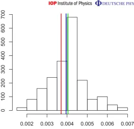
[image:9.595.147.411.89.343.2]700
Figure 1. Histogram of the norm-two error kρ− ˆρk22 of the MLE ρˆ for 100
samples from a fixed pure state ρ. The mean square error (green line) is very close to the classical Cram´er–Rao bound (blue line) as predicted by asymptotic theory, and the latter is only slightly larger than the ‘quantum optimal bound’ (red line), showing that for pure states the ions measurement is almost almost optimal amongallmeasurements.
(green line) is very close to the asymptotic prediction (blue line) computed from (10) which is equal to 3.9×10⁻³. More interestingly, we find that the MSE is also very close to the ‘quantum optimal bound’ (red line) which describes the best MSE achievable withanymeasurement! The latter can be obtained by using the machinery of quantum Cram´er–Rao theory and is given by the simple formula (see [64] and references therein)
QMSE= ]parameters] samples =
2(2k
−1) 3kn =
2(24−1)
34×100 =3.7×10
−3.
(11)
3.1. Mean square error (MSE) of the naive estimator
With the square error defined as in (7), we note that the MSE of each coefficient ρˆi for which i1, . . . ,ik 6=0, is of the order 1/(n·2k) since we are essentially dealing with the problem of estimating the mean of a random variable with values {+2−k/2,
−2−k/2
}. Therefore these coefficients alone (not counting those for which some ij are zero) bring a contribution of the order 3k/(n·2k) which is larger than QMSE (11) by a factor (9/4)k/2. For the particular example ofk =4 and n=100 this gives an MSE of 5×10⁻² which is an order of magnitude larger than that of the MLE.
3.2. MSE of the coarse grained data
At this point, it is natural to ask the following question. Suppose that we are given the 3k empirical averages of the Pauli productsσi
ˆ
ρi≈Tr(ρσ˜i)= hψ| ˜σi|ψi, i1, . . . ,ik6=0 (12)
which are obtained by computing one empirical average for each column of the original dataset. Is there a more efficient method to estimate the pure state |ψi, from the data (12) and what is its MSE? Two important candidates are thecompressed sensingandlassoalgorithms [46] (with the slight difference that they would use a smaller number of settings, but proportionally more measurements per setting). Both methods aims at estimating the state by trying to match the empirical expectations ρˆi with those of a selfadjoint matrix, while at the same time penalizing the trace norm of the matrix. Testing these methods is beyond the scope of this paper, but the asymptotic efficiency theory offers a shortcut to the answer of the above question. Applying the same methodology as before, but to the coarse grained data (12) we can predict that (asymptotically) the MSE of any estimator is bounded from below by that of the MLE ρˆcg
which in turn satisfies
lim
n→∞nE k ˆρcg−ρk
2 2
=Tr(G(θ)Icg(θ)−1), (13)
where the only difference with (11) is the Fisher information matrix which satisfies the inequality Icg(θ)6I(θ). Figure 2 shows histograms of the asymptotic MSE (11) for the full MIT data (left panel) versus the MSE (13) of the coarse grained data (right panel). The histograms were produced with 250 randomly chosen pure states, k=4 and n=100. Note that the MSE of the coarse grained data is smaller than the (partial) estimated contribution of the naive estimator. However, the MSE is still an order of magnitude higher that that of the full dataset, due to the fact that a significant amount of information has been discarded in the process of retaining the Pauli products expectations.
To summarize, we conclude that MIT works because the different settings ‘overlap’ with each other in the sense that the one dimensional projections |esdiheds| form an overcomplete set of size 2k
MSE
F
requency
0.00388 0.00392 0.00396
01
0
2
0
30
40
5
06
0
MSE
Frequency
0.03 0.04 0.05 0.06 0.07 0.08
02
0
40
60
8
01
0
01
[image:11.595.145.532.86.291.2]20
Figure 2.Histograms of asymptotic MSE’s for 250 randomly chosen pure states, with k=4 and n=100. Left panel: full counts dataset. Right panel: coarse grained dataset. Keeping only the empirical means of the Pauli products leads to a 10-fold increase in the MSE.
sensing and lasso are found to performbetterthan ML on datasets of the type (12). This apparent contradiction is lifted by the following observations:
(1) Our comparison is between the MSE of efficient estimators for two different types of data. Based on this we conclude that any estimator using the coarse grained data will asymptotically underperform ML based on the full counts experimental dataset.
(2) The comparison in [46] is different; it regards the performance of ML versus compressed sensing and lasso for the coarse grained data. Since a completely unknown state is not identifiablefor the coarse grained model, the MLE is not consistent, and arguably should not be used in this case.
4. Model selection for quantum tomography
In the previous sections we discussed the extreme scenarios of ‘full’ quantum tomography and estimation of pure states. In reality, the states produced in experiments tend to have one or few significant eigenvalues and a large number of small eigenvalues of different orders of magnitude, which account for the imperfections in the preparation procedure. Therefore, neither of the two settings seem to be suitable: the former underfits the real state while the latter overfits by trying to estimate eigenvalues that may not be statistically significant.
suitable for describing the data. Our aim is to apply the model selection methodology to state tomography, the models being the families of states of a given rank. The same methods can be used in tasks such as quantum homodyne tomography [34] where the state to be estimated is that of a light pulse (one mode continuous variables system), and a model could be the set of states with a given maximum number of photons [65].
To select the rank of the state we will use two well established methods: the AIC [50] and the BIC [51]. Both methods amount to penalizing the log-likelihood function by a factor proportional to the dimension of the model, and choosing the MLE with the smallest value of the information criterion. In the next section we give a brief general description of AIC and BIC, after which we discuss the parametrization of the fixed rank quantum models, and the implementation of the model selection procedure.
4.1. Akaike information criterion (AIC) versus Bayesian information criterion (BIC) model selection
Occam’s razor is an old scientific principle which states that when trying to explain a phenomenon, one should choose the simplest model that adequately fits the data. A very complex model will be able to fit the given data almost perfectly but it will not be able to generalize very well. On the other hand, very simple models will not be able to describe the essential features of the data. Therefore, we must make a compromise and choose a model which is as simple as possible, but no simpler. It is not surprising that many approaches have been proposed over the years for dealing with this key aspect in statistical modelling.
The general framework of model selection is the following. We are given n samples
X= {X1, . . . ,Xn} from some unknown distribution P which we try to fit with a distribution from one of several possible statistical models
Mr := {Pθr :θr ∈2r ⊂R
p(r)
}, r=1, . . . ,D,
whereMrhas a parameterθrof dimension p(r). For simplicity we assume that Xi ∈ {1, . . . ,a} are discrete random variables, as in the case of MIT measurements. We also assume that at least one of the Dmodels contains the true distribution, or at least gives a reasonable approximation to it. We denote by θˆr the MLE for the model Mr, and by `θr =`θr(X):=
Pn
i=1logPθr(Xi)
log-likelihood function atθr.
4.1.1. Akaike information criterion. The AIC for modelMr is [50] AIC(r)= −2`bθr + 2p(r),
and the chosen model is the one with the minimum AIC. Since p(r)is larger for more complex models, the AIC formally biases against overly complicated models. Although the derivation of AIC is outside the scope of this paper, we briefly explain the idea behind the choice of penalty. Having computed the MLEs for different models we would like to select the ‘best’ one in the sense that the corresponding distribution Pθˆ
r is the closest to the ‘truth’ P with respect to the
Kullback–Leibler distance (or relative entropy)
K(P|Pθˆ r):=
a
X
i=1
P(i)log(P(i))−
a
X
i=1
P(i)log(Pθˆ
r(i)).
term, which nevertheless still depends on P. If instead of θˆr we had a fixed parameter θr, this term would be the expected value of the log-likelihood atθrand could be estimated by`θr(X)/n,
by the law of large numbers. However`θˆr(X)/n is a biased estimator of the second term, due to the fact that the data has been already used in computing θˆr. Akaike showed that under the regularity conditions required by the asymptotic normality theory, the bias is approximately p(r)/n, so that ML which is the closest to the truth is approximately given by the minimizer of the AIC.
4.1.2. Bayesian information criterion. The BIC for modelMr is defined as [51]
BIC(r)= −2`θˆ
r +p(r)log(n),
wherenis the sample size. Note that the BIC differs from the AIC only in the second term which increases withn, so that BIC favours simpler models (that is models with a smaller number of parameters) compared to AIC. But despite the superficial similarity between the AIC and BIC the latter is derived in a very different way, within a Bayesian framework.
For simplicity, suppose that there are two competing models,M1andM2with parameters θ1 and θ2 respectively. One begins by assigning prior probabilities q1 and q2=1−q1 to the
event that the observed data have been generated from either model. One also assigns prior distributions π1(θ1)andπ2(θ2)to the model parameters in each model. Then one can compute
the marginal likelihoods which can be interpreted as the probability of observing the data if modelMi is correct, having integrated out our ignorance about the parametersθ1andθ2in each
model. Hence, one can apply Bayes theorem to evaluate the probability of modelMi being the true model given the observed data. A measure of the extent to which the data support model
M2overM1is given by theposterior odds
P(M2|X)
P(M1|X)
= P(X|M2)
P(X|M1)
q2
q1.
The first fraction on the right-hand side is called the Bayes factor and the second is known as the prior odds. The Bayes factor is a fundamental quantity in Bayesian theory and can be interpreted as a measure of the extent to which the data support model M2 over M1 when the prior odds are equal to one. The difference BIC(1)−BIC(2)can be shown to be a large sample approximation to the logarithm of the Bayes factor, so that the second model is chosen if the difference is positive.
4.2. Parametrizing models with fixed rank
Here we describe the fixed rank models which will be used in model selection. LetD(d,r)be the set of rankr states of ad-dimensional quantum system, i.e. those states which have exactly r non-zero eigenvalues, and let
R(d,r):=
r
[
i=1
D(d,r)
be the set of states of rank at mostr. Every stateρhas a unique spectral decomposition
ρ=
r
X
where λi >0 are its distinct eigenvalues, and Pi is an eigenprojector whose dimension is equal to the multiplicitymi ofλi. The spectral information (λ1,P1, . . . , λr,Pr)can be used to construct a parametrization ofD(d,r)andR(d,r), which has the advantage of a direct physical interpretation. However, the practical implementation of such a parametrization for computing the MLE is less straightforward due to the orthogonality constraints for the eigenvectors, and the singularities appearing on lower dimensional manifolds consisting of states with non-trivial sets of multiplicities. A variation on this would be to parametrize the state by the set of eigenvalues and an eigenbasis, in which case the singularity problem is replaced by the non-identifiability of the different basis vectors corresponding to the same eigenvalue.
We will describe an alternative parametrization which is related to the Cholesky factorization of the state. Recall that any positive definite matrix A∈M(Cd) has a unique decomposition
A=T∗T, (14)
where T is an upper triangular matrix with strictly positive diagonal elements. Therefore there exists a one-to-one correspondence between full-rank states ρ and matrices T as described above, with the additional constraint
Tr(T∗T)=X i j
|Ti j|2=Tr(ρ)=1. (15)
We parametrize such a matrixT by the vector of real numbersθ :=(R,I,D)∈Rd2−1with
R:=(Re(T12), . . . ,Re(Td−1,d)),
I :=(Im(T12), . . . ,Im(Td−1,d)),
D:=(T22, . . . ,Tdd),
(16)
such that R,I are the real and imaginary parts of the off-diagonal elements ordered from the first to thed−1 row, and from left to right along each row. By (14) and (15),θ must satisfy the constraints D>0 andkRk2+kIk2+kDk2<1, and the left-top element ofT is equal to
T11=T11(θ)=(1− kRk2+kIk2+kDk2)1/2>0.
The Cholesky parametrization of the full rank matrices can be extended, albeit with some caveats, to the spaces of rank-deficient matrices D(d,r)and R(d,r). The idea is to consider a decomposition as in (14), but with T belonging to the setT+(d,r)ofd×d upper triangular matrices with the bottomd−r rows equal to zero, and satisfyingT11, . . . ,Trr >0; equivalently, one can considerr×dtrapezoidal matrices obtained by removing the zero lines of the triangular matrices. Since every T ∈T+(d,r)is of rankr, this guarantees that the corresponding stateρ has the same property. However, not all states of rankr can be decomposed in this way! Indeed it is easy to verify that ifρ=T∗T then ther×r top-left principal minor ofρmust be of rank k, and therefore such a parametrization excludes states in D(d,r) which do not satisfy this property. Nevertheless, ‘generic’ matrices of rank r dohave principal minors of rankr, in the sense that those with smaller rank principal minors form a lower dimensional subset ofD(d,r). If we restrict our attention to the subsetD(d,r)+⊂D(d,r)which excludes the ‘deficient’ states,
we find that the Cholesky decomposition exists and is unique, so that
D(d,r)+:= {ρ=T∗T :T ∈Td+,r} ⊂D(d,r).
r-lines upper triangular matrices, with non-negative elements on the diagonal. In this case, the rootT not only exists but is in general not unique.
Let 2(d,r)+ be the set of real parameters θ:=(R,I,D) of a matrix T =Tθ ∈T(d,r)+ which are defined similarly to equation (16), and let2(d,r)be the set of parameters associated to matrices inD(k,r). We define twosequencesof quantum statistical models:
Q+(d,r):= {ρθ =Tθ∗Tθ :θ ∈2(d,r)+}, r =1, . . . ,d, (17)
Q(d,r):= {ρθ =Tθ∗Tθ :θ ∈2(d,r)}, r =1, . . . ,d, (18)
the first one consisting of rankrmatrices with rankr principal minor, the second one describing (albeit not always uniquely) all matrices of rank up to r. The reason why we mention the two models is that each has some appealing features and some disadvantages. For Q(d,r)the advantage is that we deal with anestedset of models
Q(d,1)⊂Q(d,2)⊂ · · · ⊂Q(d,d).
The disadvantage is that the Cholesky parametrization is not one-to-one in this case. On the other hand, Q(r,d)+ offers a one-to-one parametrization of rankr matrices inD(d,r)+, with
the disadvantage that the models are not nested, but instead Q(d,r)+ lies on the boundary of Q(d,r+ 1)+. While these facts are relevant to a theoretical analysis, for practical purposes the
distinction between the two models is less important, and in all our numerical experiments we used the modelsQ+(d,r).
4.3. The implementation of AIC and BIC model selection for rank-based models
We return now to the state estimation problem, and describe how AIC and BIC model selection is applied to the family of rank-based models described above for a system consisting ofkions, i.e.d=2k. Let
`θ =`θ({N(s|d):s∈Ok,d∈Dk}):=
X
s,d
N(s|d)logPρθ(s|d)
be the log-likelihood of the measurement data, ignoring the constant factorial terms. The MLEs ˆ
θr andρˆr for the modelQ(2k,r)+are
ˆ
θr:=arg max
θ∈2(2k,r)+`θ, ρˆr :=ρθˆr.
In order to choose between the different models we compute the AIC and the BIC for each rank and select the model with the smallest value. In our case the two criteria are given by
(
AIC(r):= −2`θˆ
r + 2p(2
k,r),
BIC(r):= −2`θˆr +p(2
k,r)
log(n·3k), (19)
with
p(d,r)=2dr−r2−1, (20)
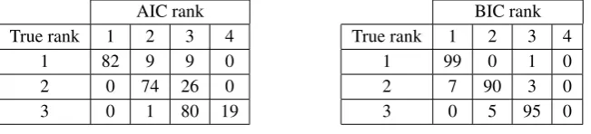
Table 1.AIC and BIC performance for 100 datasets generated by three randomly chosen states of ranks 1, 2 and 3. The tables shows the number of times AIC and BIC choose rank 1, 2 or 3 for each state.
AIC rank
True rank 1 2 3 4
1 82 9 9 0
2 0 74 26 0
3 0 1 80 19
BIC rank
True rank 1 2 3 4
1 99 0 1 0
2 7 90 3 0
3 0 5 95 0
is that the likelihood function is not concave as in the full rank model, and may have several local maxima.
To implement the ML estimation numerically, we used a standard maximization routine of the statistics package R. Additionally, we developed an array of statistical analysis tools such as Fisher information, square errors, bootstrap, Pearson χ2 statistic which will be made available online. Although the computation of the log-likelihood was optimized for faster speed, the maximization can probably be improved significantly by using more sophisticated routines. In the next sections we will discuss the results of several investigations on the performance of BIC and AIC model selection, using simulated and real data.
5. Study 1: randomly chosen low rank states
In a first simulation study we chose three ‘random’ states of ranks 1, 2, and 3 of k=4 ions, and generated 100 datasets from each state, each dataset withn=100 measurement repetitions. We then computed the MLEs for the ranks between 1 and 4 and used AIC and BIC to select the optimal rank. The exact procedure used to generate ‘random’ states is not very important, but it will be relevant that all non-zero eigenvalues of the states are significant. As illustrated in table1, BIC selected the correct rank for each state in roughly 90% of the cases while for AIC the rate is about 80%. Due to the different penalties, the AIC tends to over-estimate the rank of the state, while BIC has a slight tendency to under-estimate it. While at first sight this may appear to be a surprisingly good performance, we will show that it agrees very well with the predictions of asymptotic theory. For illustration, we consider the state of rank r =2 denoted
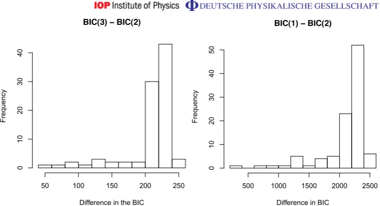
ρ, and show that the distributions of BIC(3)−BIC(2)and BIC(1)−BIC(2)concentrate on the positive axis, so that BIC chooses the correct rank. Since their behaviours are determined by different mechanisms, we will study each BIC difference separately. A similar analysis can be performed for AIC.
In the first case,
BIC(3)−BIC(2)= −2(`θˆ3−`θˆ2)+ log(n·34)(p(4,3)−p(4,2))
= −2(`θˆ
3−`θˆ2)+ 242.98, (21)
so the problem is to show that thelog-likelihood ratio statistic
3:=2(`θˆ
3−`θˆ2)
Difference in the BIC
Frequency
50 100 150 200 250
0
10
20
30
4
0
Difference in BIC
Fr
e
quen
c
y
500 1000 1500 2000 2500
01
0
2
0
30
40
[image:17.595.148.530.90.297.2]50
Figure 3.Histogram of BIC differences for the rank 2 state. Left panel BIC(3)− BIC(2); right panel BIC(1)−BIC(2). The values are in good agreement with the asymptotic predictions.
is not directly applicable here since the rank 2 model lies on the boundary of the rank 3 one, due to the positivity constraints. Nevertheless, Wilks’ theorem can be extended to more general situations where the two hypotheses can be ‘linearized’ locally (see [66, chapter 16]), in which case the limiting distribution depends on the local geometry of the two models and the Fisher information at each point. We will not pursue this analysis here but limit ourselves to giving a stochastic upper bound to the limiting distribution which will be sufficient for our purposes. The idea is to note that
3:=2(`θˆ3−`θˆ2)62(`θ˜3−`θˆ2), (22)
where`θ˜r is the ‘unconstrained’ MLE obtained by maximizing over the spaceD˜(d,r)⊃D(d,r)
consisting of matrices ρ of rank r which are not necessarily positive but must respect the property thatPρ(·|d)is a probability distribution for eachd. The unconstrained MLE is easier to analyse theoretically and can be used to explain why MLE often produces rank deficient states when the true state has high purity [12]. Now, assuming that we are in the generic situation where all probabilities for the true rank-two stateρare non-zero, this means that locally around
ρ the rank two model is a regular submodel of the extended rank 3 model, and we can apply Wilks’ theorem to conclude that
2(`θ˜
3−`θˆ2) L
−→χ2(p(4,3)−p(4,2)).
From (22) we get that 3 is stochastically bounded from above by χ2(27) and similarly
BIC(3)−BIC(2)is bounded from below by 242.98−χ2(27)which agrees with the simulations
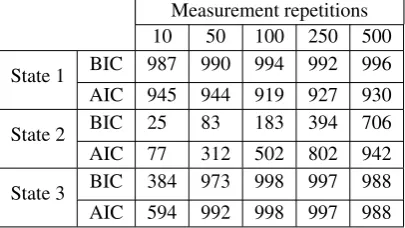
Table 2. Performance of BIC and AIC model selection for three states: pure (state 1), almost pure (state 2), and mixed (state 3). For each choice of number of repetitions, we record the number of times the BIC and AIC select thecorrect rank out of a total of 1000 simulations.
Measurement repetitions
10 50 100 250 500
State 1 BIC 987 990 994 992 996 AIC 945 944 919 927 930
State 2 BIC 25 83 183 394 706
AIC 77 312 502 802 942
State 3 BIC 384 973 998 997 988 AIC 594 992 998 997 988
not dominated by the complexity penalty but by thebiasof the lower rank model with respect to the ‘correct’ one, and in particular the distribution of the difference is state dependent. The key is to observe that while the rank 2 MLE ρˆ2 converges to the true state ρ, the rank one
MLEρˆ1converges to the stateρ1∗whose corresponding distributionPρ∗
1 is the closest to the true
distributionPρ with respect to the relative entropy (or Kullback–Leibler divergence)
ρ∗
1 :=arg min τ∈D(24,1)
K(Pρ|Pτ).
In conjunction with the law of large numbers we then obtain the almost sure convergence
3
2n = 1
n `θˆ2−`θˆ1
−→K PρPρ∗
1
asn→ ∞.
For our particular example we used one of the rank one MLEs to compute an approximate value K(Pτ|Pρ)≈11.33 which gives an estimate
BIC(1)−BIC(2)= −2(`θˆ
1−`θˆ2)+ log(n·3
4)(p(4,1)
−p(4,2))
≈2×11.33×100 + log(100×34)(p(4,1)−p(4,2)) ≈2266−261=2005,
in agreement with the histogram illustrated in the right panel of figure3.
In conclusion, for low rank states with eigenvalues which are not very close to zero, the BIC and to lesser extent AIC, identify the correct rank with high probability, the latter having a tendency to overfit the true model. On the other hand, as we will see in the next section, the BIC may underfit the true model when one or more eigenvalues are small.
6. Study 2: one ion simulations
0 100 200 300 400 500
0
.00
0.02
0.04
0.06
0.08
0 100 200 300 400 500
0.
00
0.02
0.
0
40
.0
60
.0
8
0.
10
0
.12
0 100 200 300 400 500
0
.0
0.
1
0
.2
0.3
0
[image:19.595.76.532.91.266.2].4
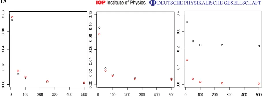
Figure 4. Mean square error for rank 1 (black circle) and rank 2 (red circle) estimators, as function of the number of measurement repetitions n= 10,50,100,250,500. Left: state 1 (pure); middle: state 2 (almost pure); right: state 3 (mixed).
samples) BIC and AIC choose the correct rank of the state, for all possible choices of states and measurement repetitions. As expected, in the case of the the pure and the mixed states both criteria require a small number of repetitions (of the order of 50) to give the correct answer. In the case of the almost pure state, we see a clear dependence withn: for small n the difference between the log-likelihoods does not off-set the complexity penalty and both criteria choose rank one; atn=500 the balance tips in favour of the rank 2 model, with AIC switching faster than BIC, on average.
Figure4shows the mean square errors (MSE) of the two MLEs MSE(r):=E(k ˆρr−ρk22), r =1,2
as a function ofn for each of the three states, with the pure state (rank one) estimator in black and the mixed state (rank two) estimator in red. For the pure state (left panel), the rank two estimator has a larger MSE due to the variance contribution from the third parameter, but the relative difference between the two MSE’s is small for all n. In this case the rank one estimator proposed by both criteria is optimal both from the point of view of parsimony, as well as estimation error. For the mixed state (right panel), the rank one estimator has a large bias which dominates the MSE, while the rank two MSE decreases at rate 1/n, as expected. At n=50 therelativedifference in risk is significant and both criteria choose the optimal rank-two estimator. The most interesting case is that of the almost pure state (middle panel). Here we see that the relative difference in MSE is not significant for small and medium number of repetitions (n=10,50,100), but for largern the error of the pure state estimator is dominated by its bias while the variance of the full state estimator becomes very small. This behaviour is picked up by the model selection criteria, which on average switch to the more complex model whenn is in the interval between 200 and 500.
6 8 10 12 14 16
1
072
4
50
1
07230
0
10721
[image:20.595.146.368.92.297.2]50
Figure 5.Log-likelihood values for the MLE as a function of rank.
in errors remains small. Finally, the BIC is more aggressive in selecting the lower complexity model, due to the additional log-factor in the penalty.
7. Study 3: model selection for four ions real data
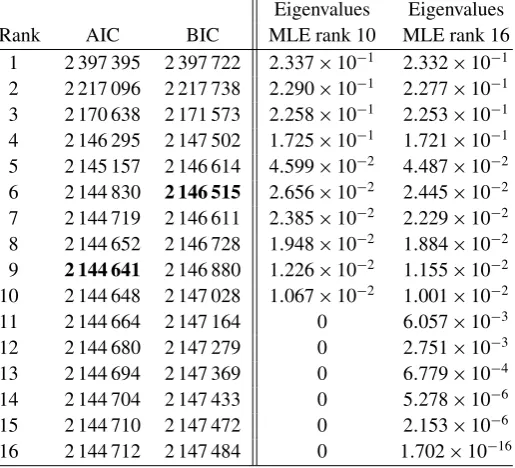
In the third study, we applied the model selection methods to experimental data provided by Rainer Blatt’s group from the University of Innsbruck. The aim of the experiment [11] was to create a particular four ions bound entangled state of rank 4 called Smolin state [67], and the measurement dataset consisted of counts for the 34 measurement settings, with a number n=4800 of repetitions for each setting. We computed the MLEs ρˆr for all ranks r between 1 and 16, and found that the corresponding log-likelihoods reach a plateau at rank 10 (see figure 5) which indicates that the rank 10 model is already sufficiently rich to describe the measurement data. Reinforcing this conclusion, we found that the value of the ML for rank 10 (and the subsequent ones) was slightlylargerthan that of that of the ML over all states computed with Hradil’s iterative method [59], probably due to the fact that the latter had not reached the true maximum after 1000 iterations.
The values of the AIC and BIC for all ranks are shown on the left side of table3. The two criteria reach minima at ranksr =6 and respectivelyr =9, as a result of the trade-off between the increasing penalty and the log-likelihood. As expected, the BIC chooses a smaller rank due to its larger complexity penalty, but both methods capture the top four eigenvalues of order 10−1
and a few of the following ones of order 10−2 which account for experimental imprecision in
Table 3.Left: values of AIC and BIC for the MLEs of ranks 1–16. The minimum values of the two criteria are attained at ranks r =9 and respectively r =6. Right: eigenvalues of the MLEs of rank 10 and 16 in decreasing order.
Eigenvalues Eigenvalues
Rank AIC BIC MLE rank 10 MLE rank 16
1 2 397 395 2 397 722 2.337×10⁻¹ 2.332×10⁻¹ 2 2 217 096 2 217 738 2.290×10⁻¹ 2.277×10⁻¹ 3 2 170 638 2 171 573 2.258×10⁻¹ 2.253
×10−1 4 2 146 295 2 147 502 1.725×10⁻¹ 1.721
×10−1 5 2 145 157 2 146 614 4.599×10⁻² 4.487×10⁻² 6 2 144 830 2 146 515 2.656×10⁻² 2.445×10⁻² 7 2 144 719 2 146 611 2.385×10⁻² 2.229×10⁻² 8 2 144 652 2 146 728 1.948×10⁻² 1.884×10⁻² 9 2 144 641 2 146 880 1.226×10⁻² 1.155×10⁻² 10 2 144 648 2 147 028 1.067×10⁻² 1.001
×10−2 11 2 144 664 2 147 164 0 6.057×10⁻³ 12 2 144 680 2 147 279 0 2.751×10⁻³ 13 2 144 694 2 147 369 0 6.779×10⁻⁴ 14 2 144 704 2 147 433 0 5.278×10⁻⁶ 15 2 144 710 2 147 472 0 2.153×10⁻⁶ 16 2 144 712 2 147 484 0 1.702×10⁻¹⁶
7.1. Pearsonχ2-test
As an additional tool for probing the conclusions of the model selection procedures, we recast the problem as that of testing between the hypotheses:
(
H0=‘the dataset is generated by a state of rank at mostr’,
H1=‘the dataset is generated by a state of rank higher thanr’.
A standard approach to such a problem is based on using the Pearson χ2-statistic. Following the general procedure described in the appendix, we consider the rankr MLEρˆr with expected number of counts E(s|d):=nPρˆr(s|d), and define the Pearsonχ2-statistic
T(r)=X
s,d
(N(s|d)−E(s|d))2
E(s|d) , (23)
where N(s|d)are the counts from the real data. Under the hypothesis H0, the Pearson statistic has an asymptotic χ2 distribution with number of degrees of freedom equal to the number of
free parameters of the dataset minus the number of parameters of the model
df(r):=34×(24−1)−p(r,4).
Therefore one can define the (asymptotically) levelαtest
(
if T 6tα: accept H0,
Parametric Bootstrap
Pearson’s Chi Square Statistic
Density
900 1000 1100 1200 1300
0.000
0.002
0.004
0.006
[image:22.595.147.388.109.327.2]0.008
Figure 6. Pearson χ2 statistic T (blue line), the limit χ2 distribution (red
curve) and the parametric bootstrap distribution for 100 bootstrap samples. The boostrap distribution is shifted with respect to theχ2due to the fact that the state
is close to the boundary of the states space and the asymptotic theory does not hold. Based on the value ofT we conclude that the hypothesis H0is not rejected for any reasonable significance level.
where the threshold tα is chosen such that P(Y >tα)=α for aχ2(df(r))-distributed random
variableY. In practice theχ2approximation works well for pure states(r=1), and small rank
states which have only a few small eigenvalues. However, if the state has a significant number of small eigenvalues, the distribution of T(r) may differ significantly from the asymptotic
χ2 distribution. We will not pursue a theoretical analysis here, but instead use bootstrap
techniques [58] to estimate the distribution ofT(r)and then perform the test with respect to the bootstrap distribution. The idea of bootstrap is to use the measurement data itself to construct a distribution which (under the hypothesis H0) approximates that of T(r), and therefore can be
used to define the thresholdtα instead of theχ2distribution. The bootstrap distributions are constructed as follows:
(1) compute the MLEρˆr and its probability distributionPρˆr(s|d);
(2) generate a large number N of independent datasets from the distributionPρˆr(s|d) of the maximum likelihood estimation;
(3) compute the MLEsρˆ1boot, . . . ,ρˆ boot
N for the bootstrap datasets;
(4) compute the Pearsonχ2statistic for each bootstrap sample and its MLE as in (23);
(5) apply theχ2test using the empirical distribution of the boostrapχ2 statistics.
rank 6 model the hypothesis H0is rejected. Therefore, the Pearson test together with the model selection criteria indicate that a good choice for the rank of the estimator is between 7 and 9.
8. Conclusions and outlook
Statistical inference has become a key tool in interpreting the measurement data in quantum engineering experiments, which require precise, efficient and informative estimation methods. However, standard full state tomography becomes unfeasible for large dimensional quantum systems [44]. In this paper we proposed model selection as a general principle for approaching state estimation problems. As in [45, 46, 49] the aim is to reduce the dimensionality of the problem by taking advantage of the ‘sparsity’ properties of quantum states in realistic experimental settings. The route to this goal is however different. The philosophy in model selection is to try to find the simplest, or most parsimoniousexplanation of the data, by fitting different models (often of increasing complexity) and choosing the estimator with the best trade-off between likelihood and complexity. Concretely, we looked at the problem of selecting the rank of the estimator, by using two well known methods: AIC and the BIC. In both cases the fit-complexity trade-off is realized by penalizing the log-likelihood of the data with a measure of complexity proportional to the number of parameters of the fixed rank model. We have tested AIC and BIC in several real data and simulation studies which we summarize here.
Pure states.We studied the performance of (rank one) ML for pure states and found a very good agreement with the asymptotic predictions based on Fisher information and the efficiency of the MLE. More interestingly, we found that the MSE is only slightly larger than the MSE of the best possible measurement predicted by quantum version of the asymptotic theory. In particular this rules out the possibility of significantly improving the MSE by means of adaptive measurement design techniques. The (asymptotic) MSE of the full counts dataset was compared to that of the ‘coarse grained’ data obtained by estimating the means of the Pauli products corresponding to each measurement setting, as used in compressed sensing algorithms [45,46]. For four ions, the latter is an order of magnitude larger than the former due to the loss of information when discarding the full counts statistics.
Study 1. For four ions states of ranks between 1 and 3 we found that both AIC and BIC identify the correct rank in 80–90% of the cases, when the smallest non-zero eigenvalue is not too close to zero. The results are explained by using the ML asymptotic theory.
Study 2. We analysed the performance of AIC and BIC as a function of the number of measurement repetitions and the purity of the state, for a toy example consisting of one ion state. With only a small number of repetitions, both methods identify the correct rank for pure and ‘pretty mixed’ states. For an ‘almost pure’ state, the model choice switches to rank 2 as the number of repetitions increases. The switching happens roughly at the point where the MSE of the ‘wrong’ rank 1 estimator becomes significantly larger that that of the correct model, indicating that model selection is only slightly suboptimal in terms of the MSE.
Study 3.We applied model selection to the four ions experimental data provided by Rainer Blatt’s group from the University of Innsbruck. The target state of the experiment was an equal mixture of four orthogonal pure states, and BIC and AIC selected rank 6 and respectively 9, with both estimators capturing the principle eigenvalues and (some of) the noisy components due to imperfections in the preparation procedure, of the order 10−2. While the BIC prediction
Overall, the numerical results indicate that model selection gives sensible answers, and can be used as an alternative to full tomography and compressed sensing. The results presented in this paper and other ongoing studies which were not included lead to the following conclusions regarding the accuracy of the rank-selected estimators in comparison to standard (full rank) MLE. The former is more accurate (with respect to the MSE) for pure states (cf sections 3 and 6), and states with eigenvalues which are well separated from zero, cf section 5. In the real data example we found that the rank 10 estimator had slightly larger likelihood that the estimator obtained by applying Hradil’s iterative method [59], which indicates that their errors are probably very similar. On the other hand, model selection can have higher MSE than standard MLE for small number of measurement repetitions when the state has several very small eigenvalues (cf section 6), due to the bias introduced by the projection onto the lower rank space. However the in-depth one ion study shows that the relative difference in MSE is not significant, with AIC being closer to MSE optimality, in broad agreement with the theoretical properties. A more general study which goes beyond the scope of this paper, should compare these and other rank selection methods, e.g. [57] based on the spectral properties of the state and the number of measurement repetitions.
In principle the rank selection method works for any state, but is designed to take advantage of the lower complexity of small rank states. The drawback is the computational complexity of finding the MLE over states of fixed rank. Therefore it would be interesting to see whether ideas from the different methods can be combined in a fast, scalable and statistically efficient estimator. A possible future direction is apply model selection to state estimation for other types of models such as classes of matrix product states, and to system identification problems. Another topic of interest is the computation of confidence intervals (error-bars). Last but not least, there is a need for a deeper theoretical understanding of the quantum tomography statistical model. We mention two important questions: how does the state’s proximity to the boundary affect the standard asymptotic theory, and how does the model behave for a large number of ions? This would hopefully lead to improved estimation algorithms and information criteria for model selection tailored to quantum tomography.
Acknowledgments
We thank Rainer Blatt’s group for providing us experimental data, and in particular Thomas Monz and Philipp Schindler for many fruitful discussions and hospitality during our visits to Innsbruck. MG’s research is funded by the EPSRC Fellowship EP/E052290/1. MG and TK acknowledge financial support from the University of Nottingham Additional Sponsorship grant EP/J501499/1.
Appendix. Pearsonχ2-statistic and Wilks’ theorem
For reader’s convenience we collect here two important results used in the paper. We refer to [58,66] for more details.
Theorem A.1 (Pearson’sχ2statistic). Let X
1, . . .Xn be i.i.d. samples from the discrete distribution Pθ over{1, . . . ,p}, whereP:= {Pθ : θ ∈2⊂Rm
E(i)=nPθ(i)be the expected counts. Then, the Pearsonχ2statistic
T :=X
i
(N(i)−E(i))2 E(i)
converges in law as n→ ∞to theχ2distribution with m degrees of freedom.
Theorem A.2 (Wilks’ Theorem). LetP := {Pθ : θ∈2=Rm
}be a sufficiently regular model and let P0 be the submodel with parameter space 20:= {θ∈2:θ1=. . .=θk =0}for some k6m. Let X:= {X1, . . . ,Xn}be i.i.d. samples from Pθ and let3 be the log-likelihood ratio statistic
3:=2 "
sup
θ0∈2`θ
0(X)− sup
θ0
0∈20
`θ0
0(X)
#
.
Ifθ∈20, then3converges in law as n→ ∞to theχ2distribution with k degrees of freedom.
In both cases, it is essential that the parameter does not lie on the boundary, in order to be able to apply the asymptotic normality theory of the MLE. This condition is violated for states whose rank is strictly smaller than that of the fixed rank model in which they are considered. Therefore care must be taken before applying these results directly, and indeed our results show that the χ2 asymptotics fail in some cases. A more refined asymptotic analysis taking
into account the boundary effects will be pursued elsewhere.
References
[1] Southwell K (ed) 2008 Quantum CoherenceNature Insight Suppl.4531003
[2] Haroche S and Raimond J M 2006Exploring the Quantum(Oxford: Oxford University Press) [3] Dowling J P and Milburn G J 2003Phil. Trans. R. Soc.A3611655
[4] Smithey D T, Beck M, Raymer M G and Faridani A 1993Phys. Rev. Lett.701244–7
[5] Resch K J, Walther P and Zeilinger A 2005Phys. Rev. Lett.94070402
[6] Zavatta A, Viciani S and Bellini M 2004Science306660–2
[7] H¨affner Het al2005Nature438643–6
[8] Altepeter J B, Branning D, Jeffrey E, Wei T C, Kwiat P G, Thew R T, O’Brien J L, Nielsen M A and White A G 2003Phys. Rev. Lett.90193601
[9] O’Brien J L, Pryde G J, White A G, Ralph T C and Branning D 2003Nature264264
[10] Riebe M, Kim K, Schindler P, Monz T, Schmidt P O, K¨orber T K, H¨ansel W, H¨affner H, Roos C F and Blatt R 2006Phys. Rev. Lett.97220407
[11] Barreiro J T, Schindler P, G¨uhne O, Monz T, Chwalla M, Roos C F, Hennrich M and Blatt R 2010Nature Phys.6943–6
[12] Blume-Kohout R 2010New J. Phys.12043034
[13] Blume-Kohout R 2010Phys. Rev. Lett.105200504
[14] Audenaert K M R and Scheel S 2009New J. Phys.11023028
[15] Khoon Ng H and Englert B G 2012 A simple minimax estimator for quantum states arXiv:1202.5136 [16] Smolin J A, Gambetta J M and Smith G 2012Phys. Rev. Lett.108070502
[17] Heinosaari T, Mazzarella L and Wolf M M 2011 Quantum tomography under prior information arXiv:1109.5478v1
[18] Buˇzek V 2004Lect. Notes Phys.649189
[19] Teo Y S, Zhu H, Englert B G, Rehacek J and Hradil Z 2011Phys. Rev. Lett.107020404