Wireless Sensor Network, 2009, 3, 171-181
doi:10.4236/wsn.2009.13023Published Online October 2009 (http://www.SciRP.org/journal/wsn/).
Research on DOA Estimation of Multi-Component LFM
Signals Based on the FRFT
Haitao QU1, Rihua WANG2, Wu QU3, Peng ZHAO4
1
Beijing University of Posts and Telecommunications, Beijing, China 2
Communication University of China, Beijing, China 3
K-Touch Corporation, Beijing, China 4
Beijing Research Institute of China Telecom Co., Ltd, Beijing, China E-mail: quhaitao2007@gmail.com
Received April 10, 2009; revised May 20, 2009; accepted May 25, 2009
Abstract
A novel algorithm for the direction of arrival (DOA) estimation based on the fractional Fourier transform (FRFT) is proposed. Firstly, using the properties of FRFT and mask processing, Multi-component LFM sig-nals are filtered and demodulated into a number of stationary single frequency sigsig-nals. Then the one-dimensional (1-D) direction estimation of LFM signals can be achieved by combining with the tradi-tional spectrum search method in the fractradi-tional Fourier (FRF) domain. As for the multi-component LFM signals, there is no cross-term interference, the mean square error (MSE) and Cramer-Rao bound (CRB) are also analyzed which perfects the method theoretically, simulation results are provided to show the validity of our method. The proposed algorithm is also extended to the uniform circular array (UCA), which realizes the two-dimensional (2-D) estimation. Using the characteristics of time-frequency rotation and demodulation of FRFT, the observed LFM signals are demodulated into a series of single frequency ones; secondly, operate the beam-space mapping to the single frequency signals in FRF domain, which UCA in array space is changed into the virtual uniform circular array (ULA) in mode space; finally, the DOA estimation can be realized by the traditional spectral estimation method. Compared with other method, the complex time-frequency cluster and the parameter matching computation are avoided; meanwhile enhances the esti-mation precision by a certain extent. The proposed algorithm can also be used in the multi-path and Doppler frequency shift complex channel, which expands its application scope. In a word, a demodulated DOA esti-mation algorithm is proposed and is applied to 1-D and 2-D angle estiesti-mation by dint of ULA and UCA re-spectively. The detailed theoretical analysis and adequate simulations are given to support our proposed al-gorithm, which enriches the theory of the FRFT.
Keywords:DOA Estimation, The Fractional Fourier Transform, UCA, ULA, LFM
1. Introduction
In various applications of array signal processing such as radar, sonar, communications, and seismology, there is a growing interest in estimating the DOA of LFM signals by dint of time-frequency analysis tools. G. Wang [1] proposed an iterative algorithm based on time-compen-sation, but the initial estimate is necessary. Using inter-polation in the spatial time-frequency distribution matri-ces (STFD’s) [2], Gershman [3] extended the signal subspace technique and estimated effectively DOA of
LFM signals, however Gershman’s approach presences model biases in addition to time consuming. The above Wigner-Ville distribution (WVD) based methods conse-quentially suffer from the disturbance of cross-terms in the presence of multi-component signals.
adap-tive filter in the FRF domain. Secondly, the separated components are demodulated into stationary signals. Fi-nally, the 1-D DOA of LFM signals can be estimated by the traditional spectrum search method. This algorithm digs two dimensional time and frequency information without the initial estimate, frequency focusing and pa-rameter partnership. With the increasing of the Sig-nal-to-Noise ratio (SNR), the MSE is quite closed to the CRB [5], for multi-component signals, cross-terms and non-linear optimize operation are also avoided.
For the UCA widely used in the third generation mo-bile communication system, the time-frequency charac-teristics of the FRFT are combined with the beamform-ing technology in FRF domain, an algorithm for the 2-D DOA estimation of the multi-component LFM signals is also proposed. Compared with other methods, the preci-sion is enhanced by a certain extent. Simulation verifies the method to be effective in the multipath and Doppler frequency shift existed complex channels.
2. Background Knowledge of FRFT
2.1. Definition and Properties of FRFT
Recently the FRFT attracts more and more attention in the signal processing society, in 1980, Namias [6] firstly introduced the mathematical definition of the FRFT. Then Almeida [7] analyzed the relationship between the FRFT and the WVD, and interpreted it as a rotation op-erator in the time-frequency plane. This characteristic makes FRFT especially suitable for the processing of LFM signals [8–9].
As a generalization of the standard Fourier transform, the FRFT can be regarded as a counterclockwise rotation of the signal coordinates around the origin in the time- frequency plane. If the traditional Fourier transform of a signal can be considered as a / 2 counterclockwise rotation from the time axis to the frequency axis, the FRFT can be accordingly considered as a counterclock-wise rotation from the time axis to the axis with an angle
u
, as illustrated by Figure 1.
The FRFT of signalx t( )is represented as
( ) P[ ( )] ( ) ( , ) X u F x t x t K t u dt
(1)where pis called the order of the FRFT,p/ 2 , denotes the FRFT operator and
[
p
F ] K t u( , ) is the
kernel function of the FRFT
2 2
1 cot exp( cot
2 2
( , ) csc ),
( ), 2
( ), (2 1)
j t u
j
K t u jtu n
t u n
t u n
(2)
( , )
s
W t f
( , )
p s
W u v
u
v
[image:2.595.330.539.507.623.2]
Figure 1. FRFT and WVD.
This has the following properties,
*
( , ) ( , )
K t u K t u (3)
* ' '
( , ) ( , ) ( )
K t u K t u dt u u
(4)Hence, the inverse FRFT is
( ) P[ ( )] ( ) ( , ) x t F X u X u K t u du
(5)Equation (5) indicates that signal x t( ) can be inter-preted as decomposition to a basis formed by the or-thonormal LFM functions in the domain, and the domain is usually called the fractional Fourier domain, in which the time and frequency domains are its special cases. The FRFT is a one-dimension linear transform and has the rotation-addition property. Essentially, the repre-sentation of a signal in the fractional domains contains the information in both time and frequency domains of the signal; Thus the FRFT is considered as a time-fre-quency analysis method and has close relationships with other time-frequency analysis tools.
u u
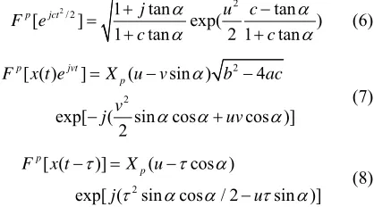
In Reference [10], some important characteristics are expressed as
2/ 2 1 tan 2 tan
[ ] exp(
1 tan 2 1 tan
p jct j u c
F e
c c )
(6)
2
2
[ ( ) ] ( sin ) 4
exp[ ( sin cos cos )] 2
p jvt
p
F x t e X u v b ac
v
j uv
(7)
2
[ ( )] ( cos )
exp[ ( sin cos / 2 sin )]
p
p
F x t X u
j u
(8)
2.2. Discrete FRFT Computation
173
x
x
x
[image:3.595.106.238.78.200.2]
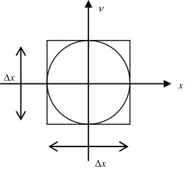
Figure 2. Normalized time-frequency support region.
different accuracies and different complexities. In this paper, we select the decomposition algorithm proposed in Reference [11]. This algorithm decomposes the putation of DFRFT to a convolution which can be com-puted by FFT, and the result is very close to the output of continuous FRFT. In this algorithm, the signal represen-tation in time domain and frequency domain should be approximately constrained with an interval of [T/ 2,
and a bandwidth of / 2]
T [F/ 2, / 2F ] respectively, viz. the time-bandwidth product of the signal is NTF, and according to the uncertainty principle, con-stantly. If the sampling rate is selected as
1
N /
s
T T N ,
the discrete representations of the signal in time domain and frequency domain will have the same length, which is called the dimensionless normalized process and the principle can be shown in Figure 2.
Therefore, Equation (1) can be expressed as
2cot 2 csc 2cot
( ) j u j ut j t ( )
X u A e e e x t d
t (9)where
1 cot 2 j A
For 0.5 p 1.5, signal has a bandwidth which is at most
2cot
( )
j t
e xt
2F and can be represented using
Shannon formula
2cot 2cot /(2 )2
( ) sin 2
2 2
N
j t j n F
n N
n n
e x t e x c F t
F F
(10) Substituting Equation (10) into Equation (9) and ex-changing the sequence of the integral and the summation, we have
2cot 2 csc /(2 ) 2cot /(2 )
( ) ( )
2 2
P
N
j u j un F j n F
n N
X u F x t
A n
e e e x
By quantizing the variable in the fractional Fourier domain, Equation (11) can be finally discredited as
u
2 2 2
( 2 )/(2 )
( )
2 2 2
N
P j m mn n
n N
A
n n
X m F x e F x
F F F
(12) where X( )m denotes the DFRFT of signal x t( ),
cot
, csc. This algorithm can be imple-mented by FFT, and has a computation complexity of
2
og N) ( lN
[11].
2.3. Two Special FRF Domain
WVD is an important non-stationary signal analysis tool, which has a very simple relationship with FRFT; viz. the WVD of FRFT is the coordinate rotation of the original signal’ WVD, while the shape of WVD keeps unchanged in the rotation. Therefore, a lot of the WVD-based signal processing methods can be substituted by FRFT. The relationship of the two time-frequency analysis tools can draw a conclusion that “time width ” and “fre-quency width(
(u) )
v
” will change with the difference of the rotation angle. Considering two extreme cases,
0,
u v
or v 0, u , from the above analysis, the former corresponds to the rotation an-gle cot1
cot
, LFM signal becomes an impact func-tion, which domain is called energy concentrated FRF one. The latter corresponds to the rotation
an-gle , LFM becomes a single
fre-quency signal, which domain is called demodulated FRF one and is the base of the proposed algorithm in this pa-per. By dint of the time-frequency rotation property of FRFT, the detection, extraction and parameter estimation of LFM signals can be easily achieved.
1
/ 2
2.4. The FRFT of Gaussian White Noise
Theorem 1: The FRFT of zero-mean Gaussian white noise is still Gaussian white noise.
Proof: let n t( )subject to the N(0,2) distribution, and N up( ) is its FRFT, the mean is
( )
p[ ( )]
p
[ ( )]
0p
E N u E F n t F E n t (13) Because the FRFT is the linear transform, does not change the distribution characteristics of Gaussian noise. Therefore, the noise is still a zero mean Gaussian noise.
2
F F
As for the second-order statistical properties of noise, the correlation of the white noise can be defined as:
( )
n t
(11)
( ) (* )
2 ( )The correlation of N up( ) is defined as:
*
* *
* *
2 *
2 *
( ) ( )
( ) ( , ) ( ) ( , )
( ) ( ) ( , ) ( , )
( ) ( , ) ( , )
( , ) ( , )
p p
p p
p p
p p
p p
E N u N u v
E n t K t u dt n K u v d
E n t n K t u K u v dtd
t K t u K u v dtd
K u K u v d
(15)
Submit Equation (2) to Equation (15), and obtain:
2 *
2
2 0.5(2 ) cot
2 2
( ) ( )
1 cot e e
2 1 cot
2 sin ( )
2
p p
j uv v j v
E N u N u v
j
d
j
v
csc
(16)Due to Equation (16), we can see that the FRFT does not change the time-domain white characteristics of noise, while noise energy does not be changed.
Assume the array noise is the zero-mean airspace one, viz. as for the array element k , the output noise is unrelated:
(kl)
( ) ( )*
( )
*( ) 0k l k l
E n t n t E n t E n t (17) The cross-correlation of the noise in FRF domain is
*
* *
( )[ ( )]
( ) ( ) ( , ) ( , ) 0
p p
k l
k l p p
E N u N u
E n t n K t u K u dtd
(18)The above equation shows, FRFT does not change the airspace white characteristics of noise. Therefore, we can draw a conclusion that FRFT does not change the statis-tical properties of Gaussian white noise, the theorem certification has completed.
Inference: as for the M antenna array element, if the
array output noise is zero mean and variance2, the
noise covariance matrix in FRF domain is:
( ) *( )
p
N p p
R E N u N u 2IM (19)
3. 1-D DOA Estimation Algorithm
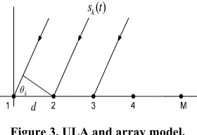
3.1. ULA Array Model
Let a ULA of M sensors receive LFM sources from
theDunknown directions{ , , , 1 2 D}, as illustrated by
d
( )
k s t
[image:4.595.354.494.78.174.2]k
[image:4.595.57.280.237.326.2]Figure 3. ULA and array model.
Figure 3. The observed signal at the output of the th sensor can be described as
i
1
( ) D [ ] ( )
i k ik
k
i
x t s t n
t (20) 1,2, , 1i M k1,2, ,D
where,
2
( ) exp[ ( / 2)]
k k k
s t j tt (21)
( 1) cos /
ik i d k c
(22)
k
, k are initial frequency and FM rate, s tk( ) is the
th source in reference sensor
k x1. is the additive
white Gauss noise with variance ( )
i
n t
2
, which is assumed to be statistically independent with signal sources. ik
is the th’s path delay, is light velocity and is sensor spacing.
k c d
From (20) and (21), we get the direction matrix is time-variant; however the traditional estimation method is merely suitable for time-invariant signal model. Therefore, the traditional method cannot be used to the direction finding of LFM signals directly.
3.2. 1-D Estimation Algorithm Description
In this section, the main work is how to make the direc-tion matrix time-invariant. The FRFT is actually a “Ro-tation” of signal in time-frequency plane. An LFM signal can be turned into an impulse in a proper fractional do-main, for the ULA model, signal s tk( )
' k
will present an impulse while the rotation angle cotk. There
will be the energy concentration, consequently a distinct peak will appear in that FRF domain, whereas the noise energy is distributed much more symmetrically in the entire time-frequency plane and will not be concentrated in any FRF domain [12].
Using (20) and (21), we get that path delay can not change the FM rates, so the impulse corresponding rota-tion angles of signal ( )s tk are same in every sensor.
Then Equation (20) is rotated with angle k' by the
FRFT from two sides:
'( )' '( )' '( )' '( )
k k k k
D
i ik il i
l k
W u Y u Y u V u
175
where, presents an impulse, and
are approximately considered as LFM signal and the white Gauss noise respectively.
'( )' k ik
Y u
) '( )' k D il l k
Y u
'( ' k i
V u
Therefore, a mask operation is applied to (23) accord-ing to the peak position , which is a narrowband filter with central frequency , and with a properly selected bandwidth , most energy of the signal
will be removed. This procedure can be re-garded as an open loop adaptive time-varying filter whose central frequency varies linearly following the peak position .
ik m ik m 2L '( )' k ik
Y u
ik m
Signal is performed the FFT (viz. FRFT of ). According to the rotation-addition property [10], the two procedures above are equivalence to one time rotation with angle
'( )' k ik
Y u
1
p
k viz.
3 / 2 cot
k k
;
tan
k k
(24) Using (6), (7) and (8), signal s tk( ) is rotated with angle
k
by the FRFT can be expressed as
2
2
( )
1 tan ( sin ) tan
exp[ ]
1 tan 2 1 tan
exp[ ( sin cos / 2 cos )]
k k
k k k k
k k k k
k k k k k
S u j u j u k 2 1 tan
exp[ ( sin cos / 2)]
1 tan
exp( cos ) exp( cos )
k
k k k
k k
k k k k
j
j
ju B ju
(25) where, 2 1 tan
exp[ ( sin cos / 2)]
1 tan
k
k k k
k k
j
B j
(26)
From (25) and (26), it can be seen that LFM signal s tk( ) has been transformed into the single frequency signal
in the FRF domain. ( )
k k
S u
Similarly, the FRFT of path delayed signal s tk( ) with rotation angle kcan be expressed as
2
2
[ ( )] exp( sin cos / 2) exp( cos ) exp[ ( cos sin )]
k
k k k
k k k k k
F s t B j
j ju
(27)
In practice, is too small viz. sin k kcos
2
exp(j sinkcosk / 2) 0 (28) Substituting (28) into (27), we get
2
2
[ ( )]
exp( cos ) exp( cos ) exp( cos ) ( )
k
k k
k k k
k k k
F s t
B j ju
j S u
k (29)
From the above analysis, Using (25) and (29), the ob-served signals described by (20) are performed the FRFT with rotation angle k from two sides
( ) ( ) ( )
k k k
ik ik ik
X u S u N u (30)
1, 2, , 1
i M
Equation (30) can be compactly represented by matrix form as follows
( ) ( ) ( )
k k k k
k k k k
X u A S u N u (31)
1
[ , , , , ]
k T
k k ik Mk
A a a a (32)
where, Tdenotes the transpose of matrix.
2
2
exp( cos )
2
exp( cos ( 1) cos )
ik ik k k
k k
a j
j i d
(33)
1 2
( ) [ ( ), ( ), , ( )]
k k k k
k k k Mk
X u X u X u X u
1 2
( ) [ ( ), ( ), , ( )]
k k k k
k k k Mk
N u N u N u N u (34)
From (32) and (33), the direction matrix k k
A is only relative to the direction information k, so the observed
signal model has been time-variant in the FRF domain. In the FRF domain, the covariance matrix of the ob-served signal can be defined as
2
[ ( ) ( )]
k k kH k k kH
XX k k k SS k
R E X u X u A R A I (35) where, H denotes the conjugate transpose of matrix.
k SS
R is the auto-correlation matrix of signal sources. The composite covariance matrix (35) has the same structure as the covariance matrix arising in the case of stationary signals. Therefore, the DOA can be estimated by per-forming eigendecomposition to k
XX
R . Using the signal
subspace k N
S and the noise subspace k N
E , the space spectrum function of the th source in the FRF domain can be given by [13]
k
( ) 1/ ( kH k kH k)
k k N N
P A E E Ak (36)
( )k
P is performed an 1-D search and kcan be obtain
by the maximal peak rotation angle. Similarly, all the Direction of LFM signals can be estimated in turn. This
k
algorithm is considered as FRFT based demodulation method.
To summarize, the proposed algorithm can be formu-lated as follows:
1) The observed signals at all sensors are rotated with a continuously variable angleby the FRFT; per-form a 2-D peak search in the( , )m plan to obtain
the maximal peak position and corresponding rotation angle
ik
m
'
k
respectively.
2) Mask operations are applied according to at every sensor, then the filtered
ik
m
2L points are
per-formed the FFT to obtain stationary signals conse-quently.
3) Get the covariance matrix of the stationary signals and perform eigendecomposition in the FRF do-main, construct the spectrum functionP( )k
ac-cording to (36).
4) Perform 1-D peak search toP( )k and obtain the
DOA of the kth LFM signal.
5) For multi-component LFM signals, all the direction can be estimated by repeating the above proce-dures.
4. 2-D DOA Estimation Algorithm Using UCA
4.1. Introduction
UCA has many advantages which the linear array cannot match. E.g. UCA can be implemented with all-direction- funding; its precision measurement does not change with the azimuth significantly and is fit for the system cor-recting. UCA is the main receiving antenna of base sta-tion system in the third generasta-tion mobile communica-tion system. Thus, the UCA based DOA estimacommunica-tion has been a research hotspot in array signal processing. Mathwes [14] proposed an UCA-RB-MUSIC method, which can be only suitable for the stationary signals; however, the actually existed signals are non-stationary ones which are represented by LFM. Tao ran [4] pro-posed an algorithm of LFM signal DOA estimation. However, the method does not apply to the UCA.
Due to the above analysis, we propose a novel DOA estimation algorithm based on FRFT using UCA, as for the multi-component LFM signals, using the characteris-tics of time-frequency rotation and demodulation of FRFT. Firstly, the observed signals are demodulated into a series of single frequency ones; secondly, operate the beam-space mapping to the single frequency signals in FRF domain, which UCA in array space is changed into the virtual ULA in mode space; finally, the DOA estima-tion can be realized by the tradiestima-tional spectral estimaestima-tion method. The proposed algorithm mines the time, fre-quency and spatial information maximally; compared
with other method, the complex time-frequency cluster and the parameter matching computation are avoided; meanwhile enhance the precision [15]. As for the multi-component LFM signals, there is no cross-term interference, the proposed algorithm is also applicable for the multi-path and Doppler frequency shift channels.
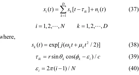
4.2. UCA Array Model
Assuming independent LFM signals and the pitch and azimuth angle is
D
1 1 2 2
{( , ),( , ), ,( , D D)} N
re-spectively, the array element number of UCA is and radius is , the center is the reference point of receiving antenna, as shown in Figure 4. Then the output of the
th sensor is: r
i
1
( ) D [ ] ( )
i k ik
k
i
x t s t n
t (37)1, 2, ,
i N k1, 2, ,D
where,
2
( ) exp[ ( / 2)]
k k k
s t j tt (38) sin cos( ) /
ik r k k i c
(39) 2 ( 1) /
i i N
(40) ( )
k
s t is the kth LFM source, and k and k are the
initial frequency and FM rate respectively, ik is the
path delay and is the light velocity. is the ad-ditive white Gaussian noise with zero mean and variance
c n ti( )
2
, which is independent with signals.
From the Equations (37) and (38), the direction matrix of observed signals is time-varying in UCA, while the traditional DOA estimation algorithm is only suitable for the time-invariant model, which cannot be used to deal with LFM signal directly.
4.3. 2-D Estimation Algorithm Description
From Equations (26) and (28), operate the FRFT to Equa-tion (37) with the rotaEqua-tion angle k from two sides:
( ) ( ) ( )
k k k
ik ik ik
X u S u N u (41)
DOA
X
Y Z
r
k
θ
k
[image:6.595.310.539.263.388.2]i
177
The matrix form of Equation (41) is:
( ) ( ) ( )
k k k k
k
X u A S u N u (42)
1
[ , , , , ]
k T
k ik Nk
A a a a (43)
where, T donates the transpose of matrix.
2
2
exp( cos )
exp( 2 sin cos( ) cos / )
ik ik k k
k k i k
a j
j r
(44)
From Equations (43) and (44), in appropriate FRF domain, direction matrix Ak is only related to angle information ,, viz. the observed signals have been transformed into unvaried smooth signal model. There-fore, the mode excitation method can be used to estimate the DOA of LFM signals.
The spatial beam former H r
F in FRF domain is de-fined as
H H
r
H
F Q CeR (45) where, H denotes the conjugated transpose of matrix.
M, , 1, ,0 1, ,Cediag j j j j jM
(46)( , , , , )
H H
M o M
R N Q Q Q (47)
Select the central Hilbert matrix,
0 '
1 [ ( ), , ( ), , ( )]
M M
Q v v v
M
(48)
0
( ) [ jM , , j , j , j , , jM ]
v e e e e e (49) '
2 /
t M
t [ M M, ] (50) where, the largest model number M kr, M'2M1. Wave number k2 / , is the initial frequency corresponding center wavelength of LFM signals. H
r F
can change the UCA in the array space into the virtual ULA in the mode space, and finally, the DOA estimation can be achieved by the eigendecomposition based search method.
Summarize the above and the main steps are as fol-lows:
1) The observed signals are continuously operated by FRFT; perform a 2-D peak search in the ( , ) m
plan to obtain the maximal peak position mik and
corresponding rotation angle k' of the k th
LFM signal respectively.
2) Select 2L points whose center is mik and
cal-culate the FFT (FRFT withp1), obtain the kth single frequency signal k( )
ik
X u .
3) Let k( )
ik
X u pass the beam switch H r F , viz.
( ) ( )
( ) ( )
k k
k k k
H
ik r ik
H H
r k r
Y u F X u
F A S u F N u
,
And calculate its covariance matrix [ k( ) k( )H]
Y ik ik
R E Y u Y u .
4) DefineRRe(RY), perform eigendecomposition to R and obtain the signal subspace S and
noise subspace G. Construct:
1 ( , )
( , ) ( , )
k k T T
ik k k ik k k
P
a GG a
,
where, ( , ) H ( , )
ik k k r k k
a F a
k
, perform 2-D spectrum search and obtain and k.
5) As for the multi-component LFM signal, repeat the above process and obtain all the DOA of signals respectively.
5. Performance Analysis and Simulation
5.1. FRFT Property Simulation
5.1.1. Simulation of FRFT and WVD
As we all know, WVD is also one of the most important and most widely used time-frequency analysis tool, which is bound to FRFT with the existence of close ties. The derivation process is relatively complex; however, there is a very simple relationship between FRFT and WVD, that is, FRFT of WVD is the coordinate’s rotation form of WVD of original signal [10].
In order to validate the relationship between the FRFT and WVD, experiments of compute simulations are given. We assume a wideband LFM signal s t( ) with a length of 1024, which is modeled as: initial frequency and FM rates are9MHz, 0.7MHz/s, sample
frequency is fs 50MHz. The WVD of s t( ) is shown in Figure 5 (a), s t( )
5
is performed the FRFT by the rota-tion angle 0.1 and get the transformed signal
. The WVD of the transformed signal
is shown in Figure 5(b). Compared the two figures, it can be found that the WVD of is just the rotation of the WVD of
0.15 ( )
S u S0.15( )u
0.15 ( )
S u
( )
[image:7.595.60.288.316.469.2]s t by angle 0.15 , meanwhile the
figure shape is invariable. So the FRFT is testified a kind of rotation arithmetic operators in the time-frequency plane.
5.1.2. Two Special FRF Domain Simulation
2
( ) exp[ ( 2)]
s t j t t , signal model is: 19MHz, 1 1400000MHz s/
. Sampling rate fs 50MHz, the
(a)
(b)
Figure 5. (a) The WVD of s( )t , (b) The WVD of S0.15π( )u .
(b)
Figure 6. (a) Energy concentration property of FRFT, (b) Demodulated property of FRFT.
concentration, as shown in Figure 6(a). The signal con-tinues to be rotated 2
ain,
in FRF domain, viz. in the demodulated FRF dom s t( ) shows the demodulated property, as shown in Figure 6(b).
5.1.3. Gaussian White Noise Simulation
Assume the complex Gaussian white noise is:
( ) (1,1024) (1,1024)
w n randn jrandn
continuous FRFT to it, the energy distrib
and perform ution of in different FRF domain is shown in Figure 7. We can see that the Gaussian white noise does not show energy concentration property in any FRF domain and can still be regarded as white noise. s theorem 1 is verified.
( )
w n
[image:8.595.72.270.76.485.2]Thu
Figure 7. Energy distribution in different FRF domain.
[image:8.595.322.522.76.272.2] [image:8.595.311.534.499.701.2]179
5.2. 1-D DOA Estimation Simulation
5.2.1. MSE and CRB Analysis
The FRFT is a 1-D linear transform [10]. In the FRF domain is approximately considered as the additive Gauss white noise. Therefore, the probability density of signal
( )
k k
N u
function k( )
k
X u represents normal
school and the corresponding likelihood function can be expressed as
2
2
1
[ ]
(2 ) ( / 2) 1
exp{ [ ] [ ]}
k
k k k k k k
k M M
H
k k k k k k
L X
X A S X A S
(51)
Using Reference [5], the CRB of the proposed method in the FRF domain can be represented as
1( )
RB
1
2 k k k k
k
H H H
2Re ( ) ( ) ( ) k ( )
H
k k k k k k k k
C
S d w I A A A A d w S k
(52) where, 2 is the noise variance and
I is unit matrix,
( ) k /
k k
d w dA dw.
Similarly, the MSE of the ed algorithm in the FRF domain can be represented as propos
1 ( )
VAR 2 1
1 2 1 1 1
11
2
[ ( )[ ( ) ]
( )] / {[ ] [ ( ) ] }
k k k k
k k k k k
H H H
MU k k k k k k
H
k XX XX k k X
d w I A A A A
d w R R A A R
where,
11 X
(53)
k XX
R is covariance matrix of the observed signals,
e MSE of the proposed method will be more and more closed to the CRB with the increasing of the sensor number and the SNR.
5.2.2. MSE and CRB Simulation
to d
u impinging from
11denotes the first row and first line element of matrix.
From (52) and (53), it can be obtain that th [ ]
In order validate the proposed metho , experiments of compute simulations are given. We ass me the ULA of
6
M D2 far field wideband
ar
LFM signals with a length of 1024, which is modeled as: initial frequency and FM rates e1200Hz,
1 900 Hz s/
; 2 200Hz , 2 300Hz s/ 0
2 70
respec-, and
angles tively.
of arri Sample fre
val are 1
quency is
0
30
s 900
f Hz
e FRF dom
, the mask snap-in. The input S
shots are 2L300 in th a NR
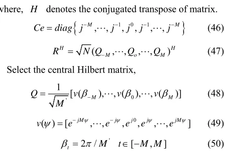
[image:9.595.322.524.61.268.2]varies fr 15dB to 29dB with an interval 2dB, at each level of the SNR, we run 100 Monte-Carlo experiments, MSE of the proposed method and original method are
Figure 8. MSE of proposed and original method.
Figure 9. MSE and CRB of proposed method.
shown in Figure 8. Obviously, the accuracy of our method has certain improvement comparing with the method proposed in the Reference [4].
[image:9.595.318.531.64.498.2]In same assumption, the input SNR various from –15dB to 6dB with an interval 3dB, 100 times Monte-Carlo simulations are performed at each level of the SNR, MSE of the first signal and CRB are shown in Figure 9. It can be seen, the MSE of proposed method is closed to the CRB even at the lower SNR.
5.3. 2-D DOA Estimation Simulation
5.3.1. 2-D Estimation RMSE Simulation 2
D two far-field LFM sources shoot the N20 0 50 ),0
1
UCA
( 3
om
the
with the angle information }. The signa
1 1
{( 60 ,
l model is:
0 0
1 0 , 1 70 )
[image:9.595.314.530.298.495.2]200Hz , 1 300Hz s/ ; 2 200Hz , 2
900Hz s/
. Sampling rate is fs 900Hz, number
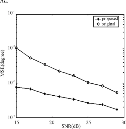
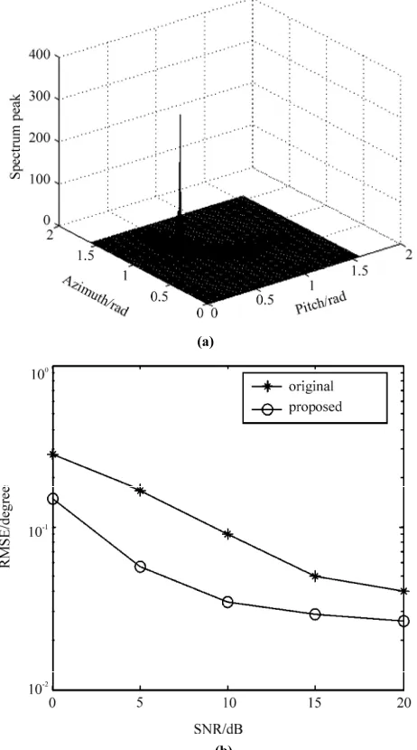
of snapshots is 1024, and the cover filter length is 2L300. The Figure 10(a) gives the 2-D DOA
tio
RMSE (root ean square error, RMSE) comparison curves of the be seen in igure 10(b). The accuracy of our method has certain
thm. estima-n of sigestima-nal oestima-ne iestima-n the 0dB SNR.
Change the input SNR range from 0dB to 20dB with the interval 5dB, firstly perform big step search to obtain the rough DOA estimation. Then run the high differen-tiation search with the 0.001rad step. Run 300 time Monter-Carlo experiment respectively, the
m
proposed algorithm and literature one can F
improvement compared to the original algori
(a)
(b)
Figure 10. (a) 2-D DOA estimation using UCA, (b) RMSE comparison curves using UCA.
5.3.2. 2-D Estimation Performances in Complex Channel and Simulation
In mobile communication system, the proposed algo-rithm is applied to the complex channel which the multi- path and Doppler shift is existed simultaneously. In the same simulation conditions, viz. the random signal source model is:
(54) where,
2
1
( ) E exp( ) exp[ ( ( ) ( ) / 2)]
k e e k e k e
e
s t M jf t j t t
1 1, 2 0.9
M M ,
1 2 2
f f
Doppler frequency shift is 0,
, multi-path delay is 10,21/ 900. When the SNR is 0dB, the simulation result of signal one
in most powerful path can be shown in Figure 11(a).
(a)
(b)
Figure 11. (a) 2-D DOA estimation in complex channel, (b
[image:10.595.58.289.270.685.2] [image:10.595.317.537.277.687.2]181
Change the input SNR range from –21dB to 0dB with the interval 3dB. Run 300 time Monter-Carlo experiment respectively, the RMSE comparison curves of signal one can be seen in Figure 11(b), which can show that the proposed algorithm is also effective in complex channel.
6. Conclusions
Analyzing the definition and characteristics of the FRFT, a novel DOA estimation algorithm has been presented the implementation of the method, mask operation is introduced to simply the filtering procedure with no ac-curacy degradation. Demodulation operation is us extend the application range of the traditional estimate method without performance loss. Compared with other methods, the veracity has certain improvement while th cross-terms and interp oided. The prop is also expanded to the timation using UCA,
addition, the pro-po
aking this method more reliable in theory and in prac-rich the principle and applicatio he optimization, the 2-D Cramer-R
2000.
. S. Zhou, “A novel method for the DOA
” IEEE Transactions on ASSP, Vol.
p. 2395– . In 37, No. 5, May 1989.
[6] V. Namias, “The fractional Fourier transform and its
ed to application in quantum mechanics [J],” IMA Journal of Applied Mathematics, No. 25, pp. 241–265, 1980. [7] L. B. Almeida, “Fractional Fourier transform and
time-frequency representations [J],” IEEE Transactions e
olation are av
2-D DOA es osed
on Signal Processing, Vol. 42, No. 11, pp. 3084–3091, 1994.
[8] Y. Q. Dong, R. Tao, S. Y. Zhou, et al., “SAR moving
target detection and imaging based on fractional Fourier which is suitable for the multi-path and Doppler
fre-quency shift complex environment. In
sed the method can be also applied to DOA estimation of LFM signals in colored noise or near-field environ-ment, which is not described in this paper.
The theoretical analyses about the error and CRB are also provided and verified by simulation results thus
fil
m
tice, meanwhile en e FRFT. As for t
n of ao
[10] R. Tao, L. Qi, and Y. Wang, “Principle and application of the fractional Fourier transform,” Tsinghua Publishing Company, Beijing, 2004.
[11] H. M. Ozaktas, O. Arikan, M. A. Kutay, et al., “Digital
th
Bound of the proposed algorithm is the further research direction.
7. Acknowledgements
The authors would like to thank the reviewers for their detailed comments on earlier versions of this paper.
8. References
[1] G. Wang and X. G. Xia, “Iterative algorithm for direction of arrival estimation with wideband chirp signals,” IEE Proceedings of Radar, Sonar, Navig, Vol. 147, No. 5, pp. 233–238, 2000.
[2] A. Belouchirani and M. G. Amin, “Time-frequency MU-SIC [J],” IEEE Signal Processing Letters, Vol. 6, No. 5, pp. 109–110, 1999.
[3] A. B. Gershman and M. G. Amin, “Wideband direction of multiple chirp signals using spatial time-frequency d tributions,” IEEE Signal Processing Letters, Vol. 7, pp. 152–155, June
4] R. Tao and Y [
estimation of wideband LFM sources based on FRFT,” Transactions of Beijing Institute of Technology, Vol. 25, No. 10, pp. 895–899, 2005.
[5] P. Stoica and A. Nehorai, “Music, maximum likelihood, and cramer-rao bound,
transform,” Acta Armamentarii (in Chinese), Vol. 20, No. 2, pp. 132–136, 1999.
[9] L. Qi, R. Tao, S. Y. Zhou, et al., “Adaptive time-varying
ter for linear FM signal in fractional Fourier domain,” Proceedings of the 6th ICSP, Posts and Telecommunica-tions Press, Beijing, pp. 1425–1428, 2002.
computation of the fractional Fourier transform,” IEEE Transactions on Signal Processing, Vol. 44, No. 9, pp. 2141–2150, 1996.
[12] L. Qi, R. Tao, S. Y. Zhou, et al., “Detection and
parame-ter estimation of multicomponent LFM signal based on the fraction Fourier transform [J],” Science in China (Se-ries E), Vol. 47, No. 2, pp. 184–198, 2004.
[13] X. D. Zhang, et al., Modern Signal Processing (Second editor), Tsinghua Publishing Company, Beijing, 2002. [14] C. P. Mathews, “Eigenstructure techniques for 2-D angle
estimation with uniform circular arrays,” IEEE Transac-tions on Signal Processing, Vol. 42, No. 9, p 2407, September 1994.