A Continuous Approach to Binary Quadratic Problems

ISSN Online: 2327-4379 ISSN Print: 2327-4352

DOI: 10.4236/jamp.2018.68147 Aug. 29, 2018 1720 Journal of Applied Mathematics and Physics

A Continuous Approach to Binary Quadratic

Problems

Zhi Liu, Zhensheng Yu, Yunlong Wang

College of Science, University of Shanghai for Science and Technology, Shanghai, China

Abstract

This paper presents a continuous method for solving binary quadratic pro-gramming problems. First, the original problem is converted into an equiva-lent continuous optimization problem by using NCP (Nonlinear Comple-mentarity Problem) function, which can be further carry on the smoothing processing by aggregate function. Therefore, the original combinatorial opti-mization problem could be transformed into a general differential nonlinear programming problem, which can be solved by mature optimization tech-nique. Through some numerical experiments, the applicability, robustness, and solution quality of the approach are proved, which could be applied to large scale problems.

Keywords

Binary Quadratic Program, Continuous Approach, NCP Function, Nonlinear Programming, Aggregate Function, Multiplier Penalty Function

1. Introduction

Binary quadratic programming (BQP) problem is a kind of typical combinatorial optimization problem, and has a variety of applications in computer aided de-sign, traffic management, cellular mobile communication frequency allocation, operations research and engineering. And many combinatorial optimization problems with constraints can be transformed into BQP problems form by cer-tain transformation, so these problems can be on behalf of kinds of important problems in combinatorial optimization. Hammer [1] pointed out that any in-teger programming problems where the objective function is quadratic or linear and the constraint condition is linear can be described as BQP problems. Glover

et al. [2] have successfully used this transformation method to transform the quadratic knapsack problem into BQP problem for solving. Considering the fea-How to cite this paper: Liu, Z., Yu, Z.S.

and Wang, Y.L. (2018) A Continuous Ap-proach to Binary Quadratic Problems. Jour-nal of Applied Mathematics and Physics, 6, 1720-1732.

https://doi.org/10.4236/jamp.2018.68147

Received: August 3, 2018 Accepted: August 26, 2018 Published: August 29, 2018

Copyright © 2018 by authors and Scientific Research Publishing Inc. This work is licensed under the Creative Commons Attribution International License (CC BY 4.0).

http://creativecommons.org/licenses/by/4.0/

DOI: 10.4236/jamp.2018.68147 1721 Journal of Applied Mathematics and Physics sibility of this transformation, BQP problem has more extensive practical appli-cation. Due to the wide application background of this problem and the difficul-ties caused by NP (Non-Deterministic Polynomial) hard properdifficul-ties, it is of great academic value to study effective algorithms for solving such problems.

Binary quadratic programming can be uniformly written in the following general

( )

{ }

T min

s.t. i i, i , 1,2, ,

f x x Qx

x l u i n

=

∈ =  (1)

where Q is a real symmetric n n× _{matrix, and the objective function can be} followed by another linear term, but it can be omitted because there is no substantial influence on the method introduced later. Of course, in the following discussion, we will mainly focus on the so-called 0 - 1 quadratic programming:

( )

{ }

T min

s.t. i 0,1 , 1,2, ,

f x x Qx

x i n

=

∈ =  (2)

However, the continuous method proposed later in this paper is also applicable to the general binary quadratic programming (1), which can be easily accomplished by simple variable transformation. It is well known that 0 - 1 programming problem will increase exponentially with the increase of the scale of the problem, and within limited computer resources and time the traditional solution method will be difficult to realize. Because of the wide application prospect and difficult characteristic of 0 - 1 programming, how to solve this kind of combinatorial optimization problem effectively has been the focus of many scholars. The classical methods for solving 0 - 1 programming problems are mainly divided into two types: accurate algorithms and random search algorithms. The accurate algorithms include implicit enumeration method, branch and bound algorithm, cutting plane algorithm, dynamic programming method, etc. Random search algorithms include genetic algorithm, simulated algorithm, artificial neural network algorithm, etc. [3] [4] [5] [6] [7]. But continuous method has become a new tendency of the 0 - 1 programming problem in recent years, whose advantage is to avoid inherent characteristics of the combinatorial optimization problem, and no longer limited to the size of the problem. This method is to transform the combinatorial optimization Aproblem into equivalent continuous optimization problem for solving, thus effectively avoid the so-called combination explosion problem, which can solve some large combinatorial optimization problems efficiently. While this approach is still in the exploratory stage with few research work in this area, but we think it is a noteworthy new research direction. Interested readers can see the literature [8]-[13].

DOI: 10.4236/jamp.2018.68147 1722 Journal of Applied Mathematics and Physics equivalent equation. Finally, the non-smooth equation is smoothed by using the aggregate function and we finally get a nonlinear smooth optimization problem.

2. Continuous Formulation of BQP

The simplest and most intuitive way to solve 0 - 1 planning problem is to adopt the round integration technology, that is, to consider 0 - 1 variable as a continuous variable, and to replace the variable constraint xi∈

{ }

0,1 , 1,2, ,i=  n in the original problem with the following interval constraint:

0≤ ≤xi 1 (3) Then a relaxation optimization problem is obtained, and the components of the relaxation solution are rounded to the nearest discrete value. Although this method is easy to implement, but the theory of this technology is not strict. It cannot guarantee that the optimal solution obtained is the global optimal solution, or even a feasible solution.

The other method is the penalty function method, which is easy to see that

{ }

0,1 , 1,2, ,

i

x∈ i= _ n _{is always equivalent to a complementarity condition:}

(

1

)

0, 1,2, ,

i i

x −x = i= _ n ₍₄₎

Therefore, the punishment function can be constructed as follows:

(

)

(

)

1

, n i 1 i

i

P α x α x x

=

=

∑

− ₍₅₎

where α >0 _{is a large enough penalty parameter. Adding this penalty function} to the object function can obtain an equivalent continuous optimization problem:

( )

T

(

)

min f x +

α

x 1−x (6)

Due to the strong concavity of

_α

_xT

(

_1−x

)

_{, the object function in (6) is} concave. The equivalence of (2) and (6) is based on the fact that the concavity function obtains the minimum value at a vertex, as well as _xT

(

_1−x

)

_{=0 has} included x=0 _and x=1 _{the sum is included. Although the vertex of the} feasible domain is not necessarily the vertex of the unit hypercube, if

α

_is sufficiently large, the global minimum can only be obtained while _xT

(

_1−x

)

_=0. However, the specific value of

α

_{cannot be determined. If the value is too} small, the penalty term will not play its role. If the value is too large, due to the strong concavity of the function, this penalty function method cannot effectively obtain the optimal solution of the original problem, so it is not an effective method. It is pointed out in literature [14], but only a new viewpoint is provided, and no more effective method is given to solve the original problem. Therefore, it is not ideal to solve the original problem directly with (6). Great-Ming Ng later constructed a logarithmic barrier term:

( )

(

)

1 ln ln 1

n

i i

i

x x x

=

 

DOI: 10.4236/jamp.2018.68147 1723 Journal of Applied Mathematics and Physics This barrier term can be used to replace the boxed constraint conditions 0≤ ≤xi 1, 1,2, ,i=  n as well as to avoid falling into the local minimum during the iteration, so as to find the global optimal solution for the original problem. At this point, the following unconstrained optimization problems can be obtained:

( )

T

(

)

(

)

1

min 1 n ln i ln 1 i

i

f x αx x µ x x

=

 

+ − −

∑

_ + − _{ (8)}

where α >0 _{is a penalty parameter and} µ >0 _{is a barrier parameter. In a} sense, (8) is an improvement on (6), but in essence they both replace

{ }

0,1 , 1,2, ,

i

x∈ i= _ n _{constraints with penalty terms or logarithmic barrier} terms.

For the BQP problem, another continuous method is proposed in this paper. Consider the following two sets of constraints:

(

)

0 1, 1,2, , ,

1 0, 1,2, , .

i

i i

x i n

x x i n

≤ ≤ =

− = =



 (9)

Obviously, these two sets of constraint conditions and binary constraint conditions are equivalent. In fact, these two constraints skillfully reform complementary constraints:

(

)

0,1 0, 1 0, 1,2, ,

i i i i

x ≥ − ≥x x −x = i= _ n ₍₁₀₎

The advantage of constructing constraint conditions in this way is that: the two constraint conditions of (9) work at the same time, and to each variable there is a unique complementary constraint condition

(

)

0,1 0, 1 0

i i i i

x ≥ − ≥x x −x =

And more importantly, complementary constraints (10) and the general constraint conditions are different: for general complementary constraints, each component is a function about x=

{

x x1, , ,2 xn

}

, and for (10), the value of

every F xi

( )

=xi

(

1−xi

)

only has relationship with the values of xi, nothing to

do with the other variables. Namely, each of the complementary constraint of (10) is independent of each other.

Through the above, the problem (2) can be equivalently transformed into the following mathematical programming problems with complementary constraints:

( )

(

)

T min

0,1 0, 1 0, 1,2, ,

i i i i

f x x Qx

x x x x i n

=

≥ − ≥ − = =  (11)

For the above complementary constraints, we can use NCP function [15] to replace them further. To better describe NCP functions, we first introduce the concept of them:

Definition (NCP function): If a function is set _φ:R2_{→R , and}

( )

a b, 0 a 0,b 0,ab 0

φ = ⇔ ≥ ≥ = _{, then the function of} φ is called an NCP function.

DOI: 10.4236/jamp.2018.68147 1724 Journal of Applied Mathematics and Physics of equation equations. Finally, we get the continuous optimization model as follows:

( )

(

)

T min

s.t. i,1 i 0, 1,2, ,

f x x Qx

x x i n

φ

=

− = =  (12)

Thus, the global optimal solution of (12) is the exact solution of problem (2).

3. Smoothing Method for BQP

According to the definition of NCP function given above, functions satisfying conditions can take various forms. Several commonly used NCP functions can be given:

( )

(

)

( )

{

}

( ) (

)

2 2

2

2 min ,

1

, min 0,

2

, 0

M

FB

a b

a b a b

a b ab a b

a b a b a a b b

φ φ

φ

φ =

= + − +

= − + +

= − − −

(13)

In the following section, we mainly choose the minimum value function to study.

It is easy to know min ,

{ }

a b = −max

{

− −a b,

}

_{, and for the non-differentiable} maximum function:

( )

{

( )

}

max max i , 1,2, ,

f x = f x i= _ n ₍₁₄₎

we often use aggregate function to carry out smooth approximation to it [16] [17]. The so-called aggregate function is a function in the following form:

( )

1

( )

1

ln expm i i

F xµ µ− µf x

=

 

= _ _ _



∑

 (15)

where the smooth parameter µ _{is large enough, and} f x ii

( )

, 1,2, ,=  n are continuous differentiable (i.e., smooth) real value function. The aggregate function has very good properties [18], which can be found from the following properties:

Lemma 3.1 The function F xµ

( )

which is defined by (15) satisfies the

following conditions:

1)

( )

( )

( )

1

max max ln

f x <F xµ ≤ f x +

µ

− m

2) _µlim_→∞F xµ

( )

= fmax

( )

x

Proof 1) F xµ

( )

can be equivalent to deformation

( )

( )

1

{

( )

( )

}

max ln 1exp max

m

i i

F xµ = f x +µ−

∑

= µf x − f x  , because

( )

max

( )

i

f x ≤ f x _{, so} 0 exp<

{

µ_f x_i

( )

− f_max

( )

x _

}

≤1_{, and there is at least one}

indicator that makes f xi

( )

= fmax

( )

x , so exist exp

{

µf xi

( )

− fmax

( )

x 

}

=1. So

we have

( )

( )

1 max

DOI: 10.4236/jamp.2018.68147 1725 Journal of Applied Mathematics and Physics Based on the above introduction, we can handle the minimum function as follows [19]:

( )

( )

(

)

(

)

(

)

(

)

1

, min , max , ,

ln exp exp

M a b a b a b F a b

a b

µ

φ

µ

−

µ

µ

= = − − − ≈ − − −

= − _ − + − _ (17)

where the smooth parameter µ is large enough, as shown by lemma 3.1, when µ → ∞_, −Fµ

(

− −a b,

)

and φM

( )

a b, are equivalent.

For ease of expression, let’s call:

(

)

{

}

(

)

1

(

)

(

(

)

)

,1 min ,1 , 1,2, ,

,1 ln exp exp 1 , 1,2, ,

M i i i i

i i i i

x x x x i n

x x x x i n

µ

φ

φ

µ

−

µ

µ

− = − =

 

− = _ − + − − _ =



 (18)

At this point, the problem (12) can be further transformed into an equivalent continuous and smooth nonlinear constraint optimization problem:

( )

(

)

T min

s.t. i,1 i 0, 1,2, ,

f x x Qx

x x i n

µ

φ

=

− = =  (19)

By this continuous method, the global optimal solution of the original problem (2) can be solved by solving the corresponding nonlinear constrained optimization problem (19). Many mature optimization algorithms have been developed for solving nonlinear equality constraint optimization problems. This paper mainly uses the multiplier penalty function method to solve the above problems (19). Multiplier method is an optimization algorithm independently proposed by Powell and Hestenes in 1969 to solve equality constraint optimization problems. Later, it was extended to solve inequality constraint optimization problems by Rockfellar in 1973. The basic idea is to start from the Lagrangian function of the original problem and add an appropriate penalty function, so as to transform the original problem into a series of unconstrained optimization subproblems.

For convenience’s sake, let’s first:

( )

(

(

)

(

)

(

)

)

(

)

(

(

) (

)

(

)

)

T

1 1 2 2

T

1 1 2 2

,1 , ,1 , , ,1

, ,1 , ,1 , , ,1

M M M n n

n n

x x x x x x x

x µ x x µ x x µ x x

φ φ φ

µ φ φ φ

Φ = − − −

Φ = − − −



 (20)

The Lagrange function of problem (19) is [20]:

( )

_,

( )

T

(

_,

)

L x

λ

= f x + Φ

λ

x

µ

₍₂₁₎

where

λ

=

(

λ λ

1, , ,2

λ

n

)

T is the Lagrangian multiplier vector, and

(

x*,

λ

*

)

is

set as KT pairs of problem (19), then it can be known from the optimality condition:

(

*_, *

)

_0,

(

*_, *

) (

*_,

)

₀

xL x

λ

λL x

λ

x

µ

∇ = ∇ = Φ = ₍₂₂₎

In addition, it is not difficult to find any x in the feasible domain is satisfied:

(

_{* *}

) ( )

_*

( )

( )

( )

_* T

(

)

( )

_*

, , ,

L x

λ

= f x ≤ f x = f x +

λ

Φ x

µ

=L x

λ

₍₂₃₎

DOI: 10.4236/jamp.2018.68147 1726 Journal of Applied Mathematics and Physics problem (19) can be equivalently transformed into:

( )

(

)

*

min ,

s.t. i,1 i 0, 1,2, ,

L x

x x i n

µ

λ

φ

− = =  (24)

Then the external penalty function method is considered to solve the problem (24). The augmented objective function is

(

)

(

)

(

)

2

( )

_T

(

)

(

)

2

, , , , , ,

2 2

L xµ L x x f x x x

α α

λ α = λ + Φ µ = +λ Φ µ + Φ µ ₍₂₅₎

In this way, we can fix λ λ= _{and find a minimum of} L xµ

(

, ,

λ α

)

, then change the value of λ _{appropriately to find a new value} x, until we get the

*

x and _λ* _{that we want. Specifically, when solving the minimum x}( )k _of

( )

(

)

min_{L x}, k ,

µ λ α in the k-th iteration of the unconstrained subproblem, the

necessary conditions for taking the extreme values are known:

( ) ( )

(

k _, k_,

)

( )

( )k

(

( )k _,

)

( )k

(

( )k _,

)

₀

xL xµ λ α f x x µ λ α x µ 

∇ = ∇ + ∇Φ _ + Φ _= (26)

And the KT-point of

(

_x*_,

_λ

*

)

_{the original problem satisfies:}

( )

*

(

*_,

)

* _0,

(

*_,

)

₀

f x x

µ λ

x

µ

∇ + ∇Φ = Φ = (27)

In order for

{ }

_x( )k _→x* _and

{ }

_λ( )k _→λ*_{, after comparing the above two}

expressions, the updating formula of the multiplier sequence

{ }

_λ( )k _is:

( ) ( ) ( )

( )

(

( ) ( )

)

1 _{,1 , 1,2, ,}

k

k k k k k

i i _µ xi xi i n

λ

+ ₌

λ

₊

α φ

_{− =}

 (28)

It can be seen from Equation (28) that the sufficient and necessary condition for

{ }

_λ( )k _{convergence is}

{

(

_x( )k_{,1 x}( )k

)

}

₀

µ

φ − → And then we proof that

( ) ( )

(

_xk ,1 _xk

)

0

µ

φ − = is also a necessary and sufficient condition for judging the KT-point

(

_x*_,

_λ

*

)

_.

Theorem 3.1 Let _x( )k _{be the minimum point of the unconstrained}

optimization problem:

( )

(

)

(

( )

)

₍

₎

2

min , , , ,

2

k k

L xµ L x x

α

λ α = λ + Φ µ ₍₂₉₎

then

(

_x( )k ,_λ( )k

)

_{being a KT-point to the (19) has a necessary and sufficient}

condition of

(

_x( )k,1 _x( )k

)

0

µ

φ − = .

Proof The necessity is obvious. The following proof is sufficient, since _x( )k _is

a minimum of (29) and

(

_x( )k ,1 _x( )k

)

0

µ

φ − = , therefore, for any feasible point:

( )

(

_, ( )k _,

)

(

( )k_, ( )k_,

)

( )

( )k

f x =L xµ λ α ≥L xµ λ α = f x (30)

that is, _x( )k _{is also a minimum of (19). On the other hand, it is noted that x}( )k

is also the stable point of (29), therefore

( ) ( )

(

k_, k_,

)

( )

( )k

(

( )k_,

)

( )k ₀

xL xµ λ α f x x µ λ

∇ = ∇ + ∇Φ = ₍₃₁₎

The above formula indicates that _λ( )k _{is the Lagrangian multiplier vector}

with respect to _x( )k _{, that is to say}

(

_x( )k _,λ( )k

)

_{is also the KT-point of (19).}

DOI: 10.4236/jamp.2018.68147 1727 Journal of Applied Mathematics and Physics multiplier method of equation constraint problem (19), the following lemmas are given by studying some properties of φµ

(

xi,1−xi

)

.

Lemma 3.2 For each i=1,2, , n, the following formula holds:

(

_,1

)

1_{ln 2}

(

_,1

)

(

_,1

)

M xi xi µ xi xi M xi xi

φ

_{− −}

µ

− _≤

φ

_{− ≤}

φ

_{− (32)}

Proof According to the properties of aggregate function:

(

)

(

)

(

)

1

max i, 1 i i,1 i max i, 1 i ln 2

f − − +x x ≤F xµ −x ≤ f − − +x x +

µ

− (33)

thus

(

)

1

(

)

(

)

max i, 1 i ln 2 i,1 i max i, 1 i

f x x

µ

−

φ

µ x x f x x

− − − + − ≤ − ≤ − − − + . That is to

say, _{min ,1}

{

}

1_{ln 2}

(

_,1

)

_{min ,1}

{

}

i i i i i i

x −x −

µ

− ≤

φ

µ x −x ≤ x −x . Therefore,

(

_,1

)

1_{ln 2}

(

_,1

)

(

_,1

)

M xi xi µ xi xi M xi xi

φ

_{− −}

µ

− _≤

φ

_{− ≤}

φ

_{− .}

Lemma 3.3 For any µ >0_{, there is}

(

)

(

)

( )

(

)

1 1

,1 ,1 ln 2

, ln 2

M xi xi xi xi

x x n

µ

φ φ µ

µ µ

−

−

− − − ≤

Φ − Φ ≤ (34)

Proof Easy to obtain by lemma 3.2 that:

(

)

(

)

1

0≤

φ

M xi,1−xi −

φ

µ xi,1−xi ≤

µ

− ln 2, so

(

_,1

)

(

_,1

)

1_{ln 2, 1,2, , .}

M xi xi µ xi xi i n

φ

_{− −}

φ

_{− ≤}

µ

− ₌

 (35)

From the above equation we know:

( )

(

)

(

)

(

)

(

)

1 2 2 1 1 2 ₂ 1 1

0 , ,1 ,1

ln 2 ln 2

n

M i i i i

i

x x x x x x

n n

µ

µ φ φ

µ µ

=

− −

 _{ } 

≤ Φ − Φ = _ − − − _ 

    ≤_{ } =  

∑

(36)

Lemma 3.4 For each i=1,2, ,_ n_, φµ

(

xi,1−xi

)

is strictly convex on the

interval

(

−∞ +∞,

)

_{; When µ ≥10}2_, 2

(

_,1

)

i i

x x

µ

φ

− _{is convex on the interval}

(

−∞,0.4737

) (

_ 0.5263,+∞

)

_.

Proof According to the definition of φµ

(

xi,1−xi

)

, it can be seen that:

(

)

{

(

)

(

)

}

(

)

{

(

)

(

)

}

1

2

2 1

,1 ln exp 1

,1 ln exp 1

i i i i

i i i i

x x x x

x x x x

µ µ

φ µ µ µ

φ µ µ µ

− −

 

− = − + −_ − _

 

− = − + −_ − _ (37)

let

(

(1 )

)

(1 )

(

(1 )

)

1 e xi e xi e xi , 2 e xi e xi e xi

r ₌ −µ −µ ₊ −µ − r ₌ −µ − −µ ₊ −µ − _{. We could get,}

(

)

(

)

(

)

(

) (

)

(

)

1 2 2 2

1 2 1 2

,1 4 0, 1,2, , ;

,1 8 4 ,1 .

i i

i i i i

x x r r i n

x x r r r r x x

µ

µ µ

φ µ

φ µ µ φ

′′ − = > =

′′ _{ }

− = _ − + − _



(38)

So φµ

(

xi,1−xi

)

is strictly convex on the interval

(

−∞ +∞,

)

; for

φ

µ2

(

xi,1−xi

)

,

when _{µ ≥10}2 _{all the x∉}

(

_{0.4737,0.5263}

)

_satisfy

(

2

(

_,1

)

)

₀

i i

x x

µ

φ

− ′′> _{, so when}

2 10

µ ≥ , 2

(

_,1

)

i i

x x

µ

φ

− is convex on the interval

(

−∞,0.4737

) (

_ 0.5263,+∞

)

_. Lemma 3.5 For any µ >0 _and α >0 _{that are large enough, as long as the}

region where x satisfies the following equation:

(

) (

2

)

(

)

2 1 4 1 2 i,1 i > 0

r r−

µ

r r +

φ

µ x −x , the augmented Lagrange function

(

, ,

)

DOI: 10.4236/jamp.2018.68147 1728 Journal of Applied Mathematics and Physics Proof Let _{l x}

( )

_,

_λ

_{=x Qx}T _{+ Φ}

_λ

T

(

_x,

_µ

)

_{then the hesse matrix of L x}

₍

_{, ,}

₎

µ λ α

is

(

)

( )

(

)

2 _{, ,} 2 _{, ,}

xxL xµ

λ α

xxl l p

α

B x p

∇ = ∇ + ₍₃₉₎

where

(

)

(

(

)

)

2

(

) (

)

, i,1 i i,1 i i,1 i , 1,2, ,

B x p =Diag_φµ′ x −x +φµ x −x φµ′′ x −x _ i=  n (40) and

(

)

(

)

(

) (

)

(

) (

)

(

)

2 2 2 1 1 2

,1 ,1 ,1

8 4 ,1

i i i i i i

i i

x x x x x x

r r r r x x

µ µ µ

µ

φ φ φ

µ µ φ

′ − + − ′′ −

 

= _ − + − _ (41)

So we just have to satisfy

(

r r2− 1

) (

2 4

µ

r r1 2

)

+

φ

µ

(

xi,1−xi

)

> 0, the matrix

(

,

)

B x p is positive, therefore for sufficiently large α >0_, L xµ

₍

, ,λ α

₎

is convex in the region that satisfies the above conditions. When _{µ >10}3 _the interval is 2

(

_,1

)

i i

x x

µ

φ

− is convex on the interval

(

−∞,0.4962

) (

_ 0.5038,+∞

)

_; when _{µ >10}4 _{the interval is}

(

_{−∞,0.4995}

) (

_{ 0.5005,+∞}

)

_.

4. Algorithm

According to lemma 3.5, we can use the augmented Lagrange penalty function to solve the problem (19). For a strictly monotonic increasing sequence

{ }

_µ

k

and

{ }

_α

k _{, the solution of unconstrained optimization min}

(

_, ( )k _, ( )k

)

n

x R∈ L xµ λ α is

{ }

_xk _{, the corresponding Lagrange multiplier is}

{ }

_λ

k _{, and is modified}

according to (28) in the iteration.

Based on the previous analysis, the basic algorithm for solving the problem (19) is as follows [19]:

Algorithm 1

Step 1 Given parameters

_µ

( )0 _{>0, α}( )0 _>0,

1 0

ε > , ε >2 0 and σ >1 1,

2 1

σ > _{. Select a starting point x}( )s,0_,λ( )0 _{and set t}( )0 _{= Φ}

(

_x( )s,0_,µ( )0

)

_{, k = 0;}

Step 2 Using BFGS algorithm solve the unconstrained minimization problem

( ) ( )

(

)

min , k , k

n

x R∈ L xµ λ α with the starting point ( )s k,

x , and denote by _x( )k _its

optimal solution;

Step 3 If

(

( ) ( )

)

( )

( )

( )

( ),

1 2

, ,

k k k s k

x µ ε f x f x ε

= Φ ≤ − ≤ _{, set x}*_=x( )k _{go to}

Step 6; else go to Step 4;

Step 4 If _{= Φ}

(

_x( )k,_µ( )k

)

_≤0,1_t( )k _{go to Step 5; else update the parameter}

( )1 ( )

1

k k

α

+ ₌

σ α

, ( )1 ( ) 2

k k

µ

+ ₌

σ µ

set k k= +1_{, and go to Step 1;}

Step 5 Set _t( )k _{= Φ}

(

_x( )k,_µ( )k

)

_{, x}(s k, 1+)_=x( )k

, modify _λ(k+1)

according to Equation (28), set k k= +1_{, and go to Step 1;}

Step 6 Finish.

The optimal solution sequence _x( )k _{required by the above algorithm makes}

( ) ( )

(

_xk ,_µk

)

DOI: 10.4236/jamp.2018.68147 1729 Journal of Applied Mathematics and Physics Then we introduce the BFGS algorithm mentioned in step 2. It is the most popular and effective quasi-newton methods at present. It was proposed by Broyden, Fletcher, Goldfarb, and Shanno independently in 1970, so it is called BFGS algorithm. We know that the basic idea of quasi-newton method is to replace the Hesse matrix _G( )l _{= ∇}2_{f x}

( )

( )l _{with one of its approximate matrixs}

( )l

B in the steps of basic Newton method, and the following relational expression is required:

( ) ( )l1 l ( )l

B s+ ₌y

(42) where displacement _s( )l _=x( )s l, _−x(s l, 1−)

, gradient difference _y( )l _=g( )l _−g( )l−1 , (42) is usually referred to as quasi-newton equation or quasi-newton condition.

Algorithm 2 (BFGS)

Step 1 Given parameters δ ∈

( )

0,1 _, σ ∈

(

0,0.5

)

_{select a starting point x}( )s l,

and positive matrices _B( )0 _{( usually set as}

_{( )}

0

G x or the unit matrix In),and

set l=0_{, f x}

( )

_{L x}

(

, ( )k , ( )k

)

µ λ α

= _;

Step 2 Calculate _g( )l _{= ∇f x}

( )

( )s l, _{, if g}( )l _{≤ε go to Step 6, output x}( )s l, _as

approximate minimum point; else go to Step 3;

Step 3 Solve the linear equations _{B d}( )l _{= −g}( )l _{and get the solution d}( )l _;

Step 4 Suppose _m( )l _{is the minimum non-negative solution that satisfies the}

following inequality: ( )

( )

_{s l, m} ( )_l

( )

( )_{s l, m}

( )

( )_l T ( )_l

f x +δ d ≤ f x +σδ g d

set _δ( )l _=δm( )l _{, x}(s l, 1+)_=x( )s l, _+α( ) ( )l_dl

; Step 5 Set _s( )l _=x( )s l, _−x(s l, 1−) _y( )l _=g( )l _−g( )l−1

,by the correction formula:

( )

( )

( )

( ) ( )

( ) ( ) ( )

( )

( ) ( )

( )

( )

( ) ( )

( )

( )

( )

( )

( )

( ) ( )

( )

( ) T

T T

1

T

T T

0

0

l l l

l _{l l l l l l}

l l l

l l l l l

B y s

B _{B s s B y y}

B y s

s B s y s

+

 _≤

  = 

 − + >

 

(43)

identify the _B( )l+1 _{, set l l= +1 and go to Step 1;} Step 6 Finish.

5. Number Experiments

About BQP questions, the current relatively popular in the question bank is J. E. Beasleys OR-library

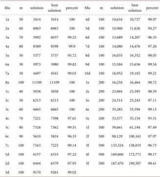
(http://people.brunel.ac.uk/~%20mastjjb/jeb/orlib/bqpinfo.html), in this paper, we has carried on the numerical experiment on parts of question bank BQP questions, and the calculation results of our continuous algorithm are compared with those of the best solution of known, as shown in Table 1.

[image:11.595.209.537.88.451.2]

DOI: 10.4236/jamp.2018.68147 1730 Journal of Applied Mathematics and Physics

Table 1. Comparison of numerical results.

Mu m solution _{solution percent} best Mu m solution _{solution percent} best

1a 50 3414 3414 100 4d 100 10,616 10,727 98.97 2a 60 6063 6063 100 5d 100 10,960 11,626 94.27 3a 70 5992 6037 99.25 6d 100 13,689 14,207 96.35 4a 80 8589 8598 99.9 7d 100 14,080 14,476 97.26 5a 50 5377 5737 93.72 8d 100 16,033 16,352 98.05 6a 30 3973 3980 99.82 9d 100 15,584 15,656 99.54 7a 30 4497 4541 99.03 10d 100 18,952 19,102 99.21 8a 100 11109 11109 100 1e 200 16,254 16,464 98.72 1c 40 5058 5058 100 2e 200 23,064 23,395 98.59 2c 50 6213 6213 100 3e 200 24,514 25,243 97.11 3c 60 6665 6665 100 4e 200 35,283 35,594 99.13 4c 70 7221 7398 97.61 5e 200 33,577 35,154 95.51 5c 80 7326 7362 99.51 1f 500 59,661 61,194 97.49 6c 90 5610 5824 96.33 2f 500 98,129 100,161 97.97 7c 100 7163 7225 99.14 3f 500 133,524 138,035 96.73 1d 100 6157 6333 97.22 4f 500 169,606 172,771 98.17 2d 100 6444 6579 97.95 5f 500 187,476 190,507 98.41 3d 100 9170 9261 99.02

It’s not hard to see from the Table 1 that in the process of solving these problems, the optimal solution obtained by our algorithm is basically close to the best known solution. Through the comparison in the table above, it can be seen that the proposed continuous algorithm is basically close to the known best solution for solving the general unconstrained 0 - 1 quadratic programming problem.

6. Conclusion

DOI: 10.4236/jamp.2018.68147 1731 Journal of Applied Mathematics and Physics leave it as a future research topic.

Conflicts of Interest

The authors declare no conflicts of interest regarding the publication of this pa-per.

References

[1] Hammer, P. and Rudeanu, S. (1968) Boolean Methods in Operations Research. El-sevier B.V., New York. https://doi.org/10.1007/978-3-642-85823-9

[2] Glover, F., Kochenberger, G., Alidaee, B. and Amini, M.M. (1999) Tabu with Search Critical Event Memory: An Enhance Application for Binary Quadratic Programs. Kluwer Academic Publisher, Boston.

[3] Goffin, J.L. (1997) Solving Nonlinear Multicommodity Flow Problems by the Ana-lytic Center Cutting Plane Method. Mathematical Programming, 76, 131-154. https://doi.org/10.1007/BF02614381

[4] Christoph, H. and Rendl, F. (1998) Solving Quadratic (0,1)-Problems by Semidefi-nite Programs and Cutting Planes. Mathematical Programming, 82, 291-315. https://doi.org/10.1007/BF01580072

[5] Wolkowicz, H. and Anjos, M.F. (2002) Semidefinite Programming for Discrete Op-timization and Matrix Completion Problem. Discrete Applied Mathematics, 123, 513-577. https://doi.org/10.1016/S0166-218X(01)00352-3

[6] Beasley, J.E. (1998) Heuristic Algorithms for the Unconstrained Binary Quadratic. Management School of Imperial College of U.K., London, 1-36.

[7] Glover, F. (2002) One-Pass Heuristics for Large-Scale Unconstrained Binary Qua-dratic Problems. European Journal of Operational Research, 137, 272-287. https://doi.org/10.1016/S0377-2217(01)00209-0

[8] Warners, J.P. (1997) Potential Reduction Algorithms for Structured Combinatorial Optimization Problems. Operations Research Letters, 21, 55-64.

https://doi.org/10.1016/S0167-6377(97)00031-X

[9] Audet, C. (1997) Links between Linear Bilevel and Mixed 0 - 1 Programming Prob-lems. Journal of Optimization Theory and Applications, 93, 273-300.

https://doi.org/10.1023/A:1022645805569

[10] Kiwiel, K.C. (2000) Bregman Proximal Relaxation of Large-Scale 0 - 1 Problems. Computational Optimization and Applications, 15, 33-44.

https://doi.org/10.1023/A:1008770914218

[11] Pardalos, P.M. (2000) Recent Developments and Trends in Global Optimization. Journal of Computational and Applied Mathematics, 124, 209-228.

https://doi.org/10.1016/S0377-0427(00)00425-8

[12] Pardalos, P.M. (1996) Continuous Approaches to Discrete Optimization Problems. Nonlinear Optimization and Applications. Plenum Publishing, New York, 313-328. https://doi.org/10.1007/978-1-4899-0289-4_22

[13] Ng, K.M. (2002) A Continuation Approach for Solving Nonlinear Optimization

Problems with Discrete Variables. Stanford University, Stanford.

[14] Horst, R., Pardalos, P.M. and Thoai, N.V. (1995) Introduction to Global Optimiza-tion. Kluwer Academic Publisher, Boston.

DOI: 10.4236/jamp.2018.68147 1732 Journal of Applied Mathematics and Physics

https://doi.org/10.1137/0131009

[16] Li, X. (1991) An Aggregate Constrained Method for Nonlinear Programming. The Operations Research Society, 42, 1003-1010.https://doi.org/10.1057/jors.1991.190 [17] Li, X. (1992) An Entropy-Based Aggregate Method for Minimax Optimization.

En-gineering Optimization, 18, 277-285. https://doi.org/10.1080/03052159208941026 [18] Li, Y. and Li, X. (2009) Continuous Approaches to 0 - 1 Programming Problem with

Applications. PhD Thesis, Dalian University of Technology, Dalian.

[19] Tao, T. and Li, X. (2006) Continuous Approaches to Discrete Optimum Design. PhD Thesis, Dalian University of Technology, Dalian.