doi:10.4236/ijcns.2011.49066 Published Online September 2011 (http://www.SciRP.org/journal/ijcns)
Parallel Minimax Searching Algorithm for Extremum of
Unimodal Unbounded Function
Boris S. Verkhovsky
Department of Computer Science, New Jersey Institute of Technology, Newark, USA E-mail: verb73@gmail.com
Received June 27, 2011; revised August 1, 2011; accepted August 25, 2011
Abstract
In this paper we consider a parallel algorithm that detects the maximizer of unimodal function f x( ) comput-able at every point on unbounded interval (0, ) . The algorithm consists of two modes: scanning and detecting. Search diagrams are introduced as a way to describe parallel searching algorithms on unbounded intervals. Dynamic programming equations, combined with a series of liner programming problems, describe relations between results for every pair of successive evaluations of function f in parallel. Properties of optimal search strategies are derived from these equations. The worst-case complexity analysis shows that, if the maximizer
is located on a priori unknown interval (n1, ]n, then it can be detected after parallel evaluations of
/ 2 1(
p
( ) 2log 1) 1
p
c n n
( )
f x , where p is the number of processors.
Keywords:Adversarial Minimax Analysis,Design Parameters,Dynamic Programming, Function Evaluation, Optimal Algorithm, Parallel Algorithm, SystemDesign, Statistical Experiments, Time
Complexity, Unbounded Search, Unimodal Function
1. Introduction and Problem Statement
Design of modern systems like planes, submarines, cars, aircraft carriers, drugs, space crafts, communication net- works etc. is an expensive and time consuming process. In many cases the designers must run and repeat expen-sive experiments, while each run is a lasting process. The goals of these experiments can be either to maximize performance parameters (speed, carried load, degree of survivability, healing effect, reliability etc.) or to mini-mize fuel consumption, undesirable side effects in drugs, system’s cost etc.
Performance parameters that are to be maximized (or minimized) are functions of other design parameters (wing span in aircrafts, aerodynamic characteristics of cars, planes, helicopters, raising cars, antennas or hy-drodynamic profiles of submarines, ships etc.). At the best, these functions are computable if CAD is applicable. Otherwise, multitude of wind tunnel experiments is re-quired for aero- or hydrodynamic evaluations. Analo-gously, numerous statistical experiments on animals and later on different groups of people are necessary if a new drug is a subject of design. Such experiments may last
months or even years. For instance, in the USA devel-opment of a new drug takes in average ten-twelve years. In view of all factors listed above, it is natural to mini-mize the number of experiments in attempts to design a system with the best parameters. In most of the cases, we can estimate an upper bound on the design parameter under consideration; yet this is not always the case espe-cially if the cost of experiments is increasing or even can be fatal in design of new drugs.
The unbounded search problem, as described in [1], is a search for a key in a sorted unbounded sequence. The goal of the optimal unbounded search is to find this key for a minimal number of comparisons in the worst case. The authors describe an infinite series of sequential algo-rithms (i.e., using a single processor), where each algo-rithm is more accurate, than the previous algoalgo-rithm. In [2] the unbounded search problem is interpreted as the fol-lowing two-player game. Player A chooses an arbitrary positive integer . Player may ask whether the in-teger
n B
x is less than . The “cost” of the searching algorithm is the number of guesses that must use in order to determine . The goal of the player is to use a minimal number of these guesses in the worst case.
n
B
ue o
n [4].
This number is a function . The author of that pa-per provides lower and uppa-per bounds on the val f
( )
c n . More results on nearly-optimal algorithms are provided in [3], and then these results are generalized for a transfinite case i
( ) c n
As pointed out in [5], the problem formulated in [2] is equivalent to the search for a maximizer of an unimodal function f x( ) , where . The goal of the search is to minimize the number of required evaluations of a function
(0, x )
( )
f x (probes, for short) in the worst case, if the maximizer is located on a priori unspecified inter-val , and where is a positive integer number. In [5], the authors consider the unbounded discrete uni-modal sequential search for a maximizer. Employing an elaborate apparatus of Kraft’s inequality, [5], inverse Fibonacci Ackermann’s function and, finally, a repeated diagonalization, they construct a series of algorithms that eventually approach lower bounds on the function .
(n1, ]n n
( ) c n
The general theory of optimal algorithms is provided in [6,7]. The problems where f is a unimodal function, defined on a finite interval, are analyzed by many authors, and the optimal algorithms are provided and analyzed in [8-12]. Optimal parallel algorithms, searching for a maxi-mum of a unimodal function on a finite interval, are dis-cussed in [13-15]. The case where f is a bimodal function is discussed and analyzed in [16-18]. The case where additional information is available is studied in [19,20]. The optimal search algorithm for the maximum of a unimodal function on a finite interval is generalized for a case of multi-extremal function in [21-23]. In all these papers, the optimal algorithms are based on the mere fact that a maximizer (minimizer) is located on a priori known finite interval (called the interval of uncertainty). The algorithms employ a procedure that shortens the interval of uncertainty after every probe. Complexities of related problems are functions of the size of interval K. Search algorithms for two-dimensional and multidimensional unimodal functions are considered respectively in [24,25].
K
K
In this paper we consider a parallel algorithm finding a maximizer (or a minimizer) of a function f defined on an unbounded interval I of Rand computable at every point xI
, )
. Without loss of generality, we assume that . It is easy to see that an algorithm, that detects a maximizer, cannot employ the same or analogous strategies as in the finite case, since the interval of un-certainty is infinite.
(0 I
Definition1.1. A unimodal function has the following properties: 1) there exists a positive number s, such that
1 ( 2) ( )
( )
f x f x f s for all 0x1x2s and
1 2
( ) ( ) ( )
f s f x f x for all sx1x2 ; 2) f x( )
is not constant on any subinterval of I. The point s is called a maximizer of function f x( ). It is not required
that f be a smooth or even a continuous function. The goal of this paper is to describe and analyze an algorithm that 1) detects an interval of length t (t-interval, for short) within which a maximizer of f is located; 2) uses a minimal number of parallel probes (p-probes, for short) in the worst case for the t-detection.
Definition 1.2. An algorithm is called balanced if it requires an equal number of probes for both stages (scanning and detection).
Definition1.3. The algorithm that is described in this paper is minimax (optimal) in the following sense. Let F be a set of all unimodal functions f F defined on I;
t be a set of all possible strategies t
S s detecting a
t-interval that contains a maximizer s of function f; and let be the number of p-probes that are re-quired for detection of the maximizer on t-interval using strategy t
( , )st N f
s . Then a minimax strategy st
detects the maximizer for a minimal number of p-probes in the worst case of the unbounded function f, [17].
The Definition 1.3 implies that
t min max
, tst St f F
N s N f s
(1.1)Remark1.1. Although s is a priori unknown to the algorithm designer, it is assumed in this paper that its value is fixed. Otherwise, the algorithm designer will not be able to provide any algorithm for t-detection of s. In-deed, the adversary can generate a function f that is in-creasing on any finite subinterval (0, )v I.
2. Choice of Next Evaluation Point
2.1. Sequential Search: Single-Processor Case
Proposition 2.1. Let us consider two arbitrary points, L and R, that satisfy inequalities 0 L R . If
( ) ( )
f L f R , then maximizer s is greater than L; if then maximizer s is smaller than R; if ( )
( ) ( )
f L f R
( )
f L f R , then s is greater than L and smaller than R, i.e., s( , )L R , [10,26].
Proof follows immediately from unimodality of the function f.
If , then a maximizer s is detected on a finite interval, i.e.,
( ) ( )
f L f R
(0, )
s R . Therefore for t-detection of the maximizer s we can employ Kiefer’s algorithm for sequential search [10,26] or the algorithm [25] for paral-lel search.
Suppose that f is evaluated at two points qi:L and :
j
q R, where 0 L R and let ( )f L f R( ). Two strategies are possible in this case: to evaluate f ei-ther at a point M( , )L R or at a point M R; {there is no reason to evaluate f at , since the Proposition 2.1 guarantees that if
q
( )
L
( )
on interval ( ,L R).
Therefore, s is either on finite interval (R,R) or on infinite interval . Keeping in mind that we consider the worst case complexity, it is reasonable to evaluate f at a point
R s
M R that is on the infinite inter-val
R,
.2.2. Multiprocessor Case
Let us consider the same function f x( ) as in the single processor case. Let us simultaneously evaluate it at points M1,,Mp, where p is the number of available
processors.
Consider four scenarios:
A: All or a part of the points M1,,Mp are inside
interval ( , )L R ;
1
B: All points M , ,Mp , ,
1
are outside interval , i.e., every point
( , )L R p
M M
[ , ]
is larger than R; C: s R R
[ , ]
; D: s R R .
2.3. Possible Outputs in the Worst Case
For both AC and AD scenarios f x( ) and can be selected in such a way that for all , for which
i
1 i p ( , )
M L M , the inequality f M( i) f( )R holds.
Hence, taking into account that we are dealing with the worst case, all evaluations must be done outside interval
if
( , )L R f L( ) f( )
q q R .
3. Optimal Unbounded Search Algorithm as
a Two-Player Game with Referee
3.1. Sequential Search: (p = 1)
Let us consider two players A and B and a referee. Their game consists of two stages.
At the beginning, player A selects a value s0 and informs the referee about it. Player B selects a value t > 0and informs player A and the referee about his choice.
At the first stage, B sequentially selects positive and distinct points 1, 2,,qi. The referee terminates the
first stage if there are points qj and qk such that j
sq and sqk.
The second stage beginsfrom state ( , ,u v w1 1 1) where
:
1 j1
u q ; v1:qj; w1:qj1.
At the second stage, B selects points and A selects in-tervals. Let the game be in state (u v wj, j, j) of the sec-ond stage. This stage terminatesif wjuj t.
Other-wise B selects a point xj vj, such that ujxjwj.
Then A eliminates the leftmost or the rightmost subin-terval, [16]. The goal of player B is to minimize the
number of points required to terminate the game. The goal of player A is to maximize the number of these points. The adversarial approach for interpretation of the optimal search algorithms is also considered in [2,27].
Remark3.1. It is easy to see that B is an algorithm designer and A is a user that selects function f and re-quired accuracy t.
3.2. Multiple-Processor Search: (p≥ 2)
An optimal parallel search algorithm with p processors has an analogous interpretation. In this case, at the first phase of the game, player B on his move selects p dis-tinct positive points. The referee terminates the first phase if there are at least two points to the right from s. At the beginning of the second phase, the player A se-lects any two adjacent subintervals and eliminates all other subintervals. In general, at the second phase, B selects points and A selects intervals. More specifically, player B on his move selects p distinct points on the in-terval and player A on her move selects any two adjacent subintervals and eliminates all other subintervals. The goal of the game is the same as in the single-processor case. It is obvious that on the first stage of the game player B must select all points in an increasing order from one p-probe to another.
Remark 3.2. At first, we will describe the optimal unbounded searching algorithm with one processing element, (PE, for short). Subsequently, we will describe and discuss the parallel minimax unbounded search with p PEs. As it will be demonstrated, the case where p is an even integer is simpler than the case where p is odd.
4. Structure of Unbounded Sequential
Search
Consider a finite interval K, i.e., its length K . In the case, if it is known a priori that sK, then we can t-detect maximizer s for at most
log K t
1o K t
probes, where
1 5
2 , [16,17]. (4.1)
However, the situation is more complicated if f is de-fined on unbounded interval In this case we divide entire interval I into an infinite set of finite subin-tervals of uncertainty 1 1
(0, ).
I
0, ] : (
I q ; I2: ( , q q1 2]; ; 1
: ( , ]
k k k
I q q ; where
1 k k
) : (
k
f f qk k
Definition 4.1. A search algorithm is in the scanning mode while for all function f satisfies inequalities .
, i.e., f is a result of the k-th probe.
1 2 k
q q q f
1 2 k
In the scanning mode we probe intervals until this mode terminates.
f f
1, 2, , k,
I I I
Definition 4.2. We say that a search algorithm is in l-th state 1 of the scanning mode if l-th
in-terval of uncertainty l l 1 l]
{ , }
l l l
p r r
( ,
I q q is to be eliminated and ql1 is the next evaluation point. Here
1: 1
l l
r q ql Il ; rl ql 1ql 1
f f
l
Remark 4.1. If l l1, then the search switches
into the detecting mode with initial state 1 , [16].
However, if l l1, then the search moves to the next 1
l state of the scanning mode. As a result, the interval
of uncertainty l1
I .
{rl, }rl f f
p
I is eliminated (since sIl1) and
the interval Il2 is the next to be examined. Since at
any state the search can switch into the detecting mode, the dilemma is whether to select interval Il2 as small
as possible (in preparation for this switch) or, if the search continues to stay in the scanning mode, to select
2 l
I as large as possible. The dilemma indicates that there must be an optimal cho e of ic Il2.
In the detecting mode, we can use an optimal strategy, [10,16,26], which locates s on t-interval. To design a minimax search algorithm, we must select all
1 2 k 1 in such a way, that the total number
of required probes on both modes is minimal in the worst case.
q q q
Definition 4.3. We say that a set of points is a detecting triplet if
( ,q q qi j, k)
i j
f f fk, where qiqjqk. (4.3) If is a detecting triplet and f is a unimodal function, then maximizer s satisfies inequality k
( ,q q qi j, k)
i
q s q, [17].
Definition4.4. In the following consideration,
means the minimal total number of required probes for both modes in order to detect maximizer s in the worst case if
( , )
U b c
( , ]
s b c .
In the following discussion, we assume that t = 1, unless it is specified otherwise.
Proposition 4.1. If f is an unimodal function and , but this is a priori unknown, then for all s is detectable after probes in the worst case, i.e.,
1
( m 1, m s F F
3
m
1]
2(m2)
m1 1, m 1
2
2U F F m (4.4) where probes are used in the scanning mode and
probes in the detecting mode. Here 1
m
3
m Fm is m-th
Fibonacci number: F1F21; FmFm2Fm1 for
m > 2.
Proof {by induction}: We will demonstrate that in the
scanning modethe optimal evaluation points
1, 2, , 1, o o o o
k
q q q qk must satisfy these properties: 1 : 1, o
q
1: o o k k k
q q F , for all k2, i.e.,
k
2 1
:
o
k i k i
q F F
2
. (4.5)Remark 4.3. First, we demonstrate how to find an ap-proximation a of s that satisfies inequality s a t, i.e.,
a t s a t. Then we will show how to adjust the algorithm, if s (n 1, ]n
( 2,F
.
1). Let s F3 42](0,1]. Consider 1q1
2 2
q . Then 1 2. Hence, Proposition 4.1 implies
that
f f
2
, ) (0
s q . Thus, aq2 2 implies that a(0,1];
therefore s a 1 t )
. It is easy to verify that, if (0,1
s and 0, then, in the worst case, two probes are not sufficient for detection of s on t-interval. Indeed, the adversary can select such s and f that satisfy the following inequalities: 1q1 s q2 and f1 f2.
Hence, in that case, s is not t-detectable on inter-val after two probes.
(0,1]
2) Let now s(Fm2,Fm12) and . Then s
can be t-detected for
mk
1
s(Fm2,Fm 2)2m1
probes. If , then kprobes were used in the scanning mode and mk
3 k probes in the detecting mode.
3) Let s(Fk11,Fk21]
1, 2, ,
i k
, but it is a priori un-known. Let for all 1,k2
: 1
i i
q F
the probes are taken in the points 2 .
In this case the following inequalities hold
1 2 k k 1 k 2
f f f f f .
Since fk fk1 fk2, then 1 2 is a
de-tecting triplet, and, as a result, the search is in the detect-ing state { 1, 2 . Then from [8,10,26], using the
optimal search algorithm, we can detect s with accuracy t = 1 for additional k evaluations of f. Hence the minimal total number of required probes for both modes is equal
(q qk, k ,qk )
}
k k
F F
1 2
( 2,Fk 2) 2
t k
U F k1. Q.E.T.
5. Optimal Balanced Sequential Search
5.1. The Algorithm
Assign a required accuracy t; {the scanning mode of the algorithm begins};
:
L t; R: 2 t; while f L( ) f R( ) do begin
:
temp L; L:R; R: R tempt; (5.1) {(5.1) generates a sequence of probing states { ,F F1 2},,
1
{Fk ,Fk}}; end;
{the maximizer s is detected: s(temp R, ); the algo-rithm is in the detecting state
{the following steps describe the optimal detecting algo-rithm-see [16]};
assign
: ;
A temp B:R; R: A B L; (5.2) repeat
if f L( ) f R( ) then
: ; : 2 ; :: ; , ;
temp L L R B B R
R temp s A R
;
;
2}
(5.3)
else
: ; : 2 ; :: ; , ;
temp R R L A A L
L temp s L B
(5.4) {(5.3) and/or (5.4) generate a sequence of detecting states {Fk1,Fk},,{ ,F F1 };
until (BA) 2t;
assign a: ( AB) 2; {a is the approximation of the maximizer: s a t}; stop.
The algorithm described above is called V-algorithm. 5.2. Optimality of Sequential Search
Proposition 5.1. The number of required probes for t-detection of a maximizer described in Proposition3.1 is minimal in the worst case.
Proof. The algorithm consists of the scanning and de-tecting modes. In the scanning mode (SM) the search is sequentially in the probing states p p1, 2,,pm where
1: 1, 2 , , m: m, m 1
p F F p F F
. (5.5) On the other hand, in the detecting mode (DM) the algorithm is in the detecting states , ,1
1
{F Fm, m}
2
{ ,F F}
{ ,
. It is known that all detecting states 1 ,
, 1 2
{F Fm, m } }
F F are optimal (there are no other strategies that can t-detect s for a smaller number of probes). At the same time the entire SM is a mirror image of the DM. Indeed, from the beginning to the end of the SM the search goes from scanning state { ,F F1 2} to scanning
state 1 , while in the DM the search goes from
detecting state { , 1 to detecting state { ,1 2
{F Fm, m }
}
m m
F F F F}.
Thus, both modes (scanning and detecting) are optimal; therefore, the entire algorithm is optimal.
6. Complexity of Minimax Sequential Search
Let us compare the optimal search algorithms for two cases:
1) Maximizer , but this is a priori un-known; here b is a positive integer;
( , m 1] s b F
2) It is known a priori that s(0,Fm)
( , . Let
be the minimal total number of required probes for t-detection of s in the worst case if
( , ) B b c
) s b c .
From Proposition 4.1, if and , then
1 1
m
bF m2
m1 1, m 1
2
2U F F m
. (6.1) However, if b0, then the following inequality holds:
0, m 1
2
2U F m
. (6.2) From [11] it follows that, if m4, then(0, m) 2
B F m , otherwise
0, m
0.B F (6.3) (6.1) and (6.3) imply that for all m4
0, m 1
2
0, m
2
2U F B F m
. (6.4) In general, if s( , ]a b (Fm11,Fm1], but this is apriori unknown, then
, 2 log
5 1
log
U a b b o b b (6.5)
where is defined in (4.1).
Equality (6.5) follows from the fact that
m m
5m
F , [13,14]. (6.6) where
1 5
2 1 , therefore limm0 if. m
Thus,
m 5
1
mF o . (6.7) If Fm1 P Fm1, then
m1 1,
2
2U F P m
. (6.8) The complexities (6.1) and (6.5) can be further re-duced if any prior information is available, [6,17], or if a searching algorithm is based on a randomized approach, [19,30].Proposition 6.1. Let be the minimal number in the worst case of the required probes to detect s on a pri-ori unknown interval
( ) c n
1,
s n n . If
1 2
m
F nFm1, (6.9)
then
2
2c n m
(6.10) Proof. First of all, the relations (6.1), (6.2), (6.5) and (6.8) are based in the previously made assumption that t := 1. From this assumption it follows that maximizer is detectable on an interval of length two, . In order to find the complexity of the algorithm if {a 1 s a 1}
1,
Case 1: If
Fm11
t n 1 and n
Fm1
t; (6.11)then (6.10) is implied by (6.5) if t :=1/2. Case 2: If
Fm1
t n
Fm1
t and
Fm11
t n 1, (6.12)
i.e., the case where
Fm11 t is in the middle of theinterval
n1,n
m.
It occurs if In this case the left half of the interval
mod 30.
n1,n
is out of interval
Fm11 ,
t
Fm1
t, i.e.,
n1,n1 /2
Fm11 ,
t Fm1
t
and, as a result, fewer probes are required for t-detection of s. However, in the worst case, the maximizer may be on the right half of interval n1,n
, hencefor both cases. For illustration see Ta-ble 6.1 below.
( ) 2( c n m2)
Thus, (6.8) implies that
2 log
2 5
1
4.c n n o n (6.13)
7. Estimated Interval of Uncertainty
In many applications, an upper bound value Q on maxi-mizer s can be estimated from a feasibility study. Let
5
T Q d Q. Here d 451.082.
Proposition 7.1. If sT , then V-algorithm re-quires fewer probes than Kiefer’s algorithm, [14]; if
T s T , then Kiefer’s algorithm and V-algorithm require the same number of probes; if , then Kiefer’s algorithm requires fewer probes than V -algo-rithm.
T s Q
Proof. Let and . Then in the
worst case
: m
T F 1
m
2 2
: m
Q F
1 1
2 2
0, 1 1, 1
0, 2 2
m m
m
U F U F F
B F m
. (7.1)
It is easy to check that the proof follows from (6.7) and from the fact that
2
2m 2 m 5 1
[image:6.595.58.285.677.718.2]F F o m . (7.2) Preliminary results on analysis of the optimal algo-rithm searching for the maximum of a multimodal func-tion on the infinite interval are provided in [28].
Table 6.1. Total number of probes as function of n.
4 n 6 494 n 798 60, 697 n 98, 208
10
c n c n 30 c n 50
8. Parallel Search: Basic Properties
If several processors are available, then, as it is indicated in [29], the algorithm can be executed in a parallel mode. [13,15] are the earliest papers on a parallel search for a maximum of a unimodal function of one variable on a finite interval, that are known to the author of this paper. Although the optimal search strategies in both papers are in essence identical, the formulation of the problem is different. The proof of optimality of the search is more detailed in [15]. [2] provides an idea of a parallel algo-rithm searching for a maximum of a unimodal function on a unbounded interval. This idea is based on an appli-cation of the Kraft’s inequality formalism, is provided in [2]. The authors indicate that the approach they used to construct an infinite series of near-optimal algorithms for the unbounded search with a single processor can be ex-panded for a multiprocessor case. However, no details are provided.
The search algorithm described in this paper is based on the following properties.
Proposition 8.1: Let us consider p arbitrary points
1, , p
q q that satisfy inequalities
1
0q qp . (8.1) If
1 2 p1 p
f f f f , (8.2) then maximizer s is greater than qp1; if
1 2 p1 p
f f f f , (8.3) then s is smaller than q2; if
1 j1 j j1 p,
f f f f f (8.4) then s is greater than qj1 and does not exceed qj1,
i.e.,
j1, j1s q q . (8.5) Proof follows immediately from unimodality of func-tion f.
9. Search on Finite Interval: Principle of
Optimality
Definition 9.1. Imp( , )u v
{ , }.u v
is a minimal in the worst case interval of uncertainty containing maximizer s that can be detected after m p-probes if the search starts from the detecting state
9.1. Properties of Imp
u v,1)
, lp
pm ,
I u v l; )
(Effectiveness of p-probes);
I u v
2)
1, 1 2 2 pm
l
,
p
5) mp
,
mp
I u v(Monot
I u v
if u1u2; v1v2; (9.2) I cu cv cI u v, for every c0; (9.5)
3)
onicity of uncertainty); (Homogeneity).
pm ,
m
, pI u v I v u ; (Symmetricity); (9.3)
9.2. Properties of
( , )
p m
I
u v
if p = 24) Imp
u v, Imq
,
Efficiency of paralu v if pq; (9.4)
( lelization); Proposition 9.1: Let uv. Then
(9.6)
(9.6) is a functional equation of dynamic programming; it implies the following property. Proofs of this and the
follow-
1 3
1 2
2 2
1 1 1 3 1 3 1 3
, 2
2 2
1 2 1 1 2 1 1 2 2
min max , max , , , max , ;
, min
min max , max , , , max , .
m m
y u y v m
m m
y y u
I u y y y I y u y v y
I u v
I y y u y y I u y y y v
ing Propositions 9.2-9.5 are provided in the Appendix. Proposition 9.2: Let uv; then
2 1 2
2 1
, if ; 2
,
, ; 0 if .
m m
m
u v
I v u v
I u v
I u z z z u u v
(9.7)
.3.Odd Number of Processors
roposition 9.3: If ; and then
9
P p2r1 uv,
2 1
1
r 1
2 1
2 1 1
, , 1 ;
,
, 1 , 1 ;
m r
m r
m
I r k vku ku r k v k k r k v u k r k
I u v
I r k v ku k u r k v r k k r k v u k
(9.8)
here for )
2
w 1 k r/
er branch of
2 (r k 1)vkuku (r k v (9.8) and for 0 k r/
in the upp
wer branch of (rk v) ku(k1)u (r k v) in the lo
(9.8).
9.4. Even Number of Processors
roposition 9.4: If
P p2r and uv, then for all
1 k r 2 the f g dynam programming
:
ollowin ic equation holds
2 1 2
2 1
1 , 1 1 , 1 1
( , )
1 , , 1 , 0 1 .
r m r
m r
m
;
I r k v ku k u r k v r k r k v u k r k
I u v
I u v r z z ku r k v z u v k
(9.9)
.5. Defining Rules of Optimal Detecting States
efinition9.2. If there exists a pair of positive numbers
and
9 2 1
2 1
1
, ,
r r
m m m m m m m
I c d I d c rd , (9.11) which means that
D
c and d such that c>d and for all non-negative numbers u and v
u v
1: ;
m m
c d dm1:cm rdm;
p is even, then
(9.12) Proposition 9.6. if
c d
p( , ) p( , ),
m m
I u v I c d (9.10) then is an op
imal detecting st
two propositions can be proved by in-du
2 2
1
, 1 ,d ,
r r
m m
I c d I c d r d
{ , }c d finitio
timal detecting state. De n 9.3. Let { ,c dk k} be the opt
ate starting from whi n be located after k addi-tional p-probes.
The following
ch s ca
ction:
Proposition 9.5. if p is odd, then
m m m m m m
which means that
1: ; 1: 1
m m m m m m
d d z c c d r d 1. (9.13)
Remark9.1. dmconst in (9.13).
1) and 2) im (9.12) and (9
op states ;
0 0
: 1; : ; : ; : 2 .
t d z c t z r p (9.14) Proposition (1) and (2) imply the defining rules optimal detecting states : if p is odd, t
if p is even, then for all
.
(9.16)
Both these rules for p odd and even can be generalized as: assign
for hen for all { ,c dk k}
1
1 1
1: ; : ;
k k k k
c r c c (9.15) k k d d 0 k
: 1c r c
1 1 1
1 1
: ;
1 1
:
k
k k k k
k
k k
d z
d d
r c rd t r z
: p 1 mod 2;
(9.17) then
1 1
1 2 k k ;
p c d
1 1
:
: mod 2 .
k
k k k
c
d p c d (9.18)
The following two examples and Table 9.1 {with t = 1;
0 0
1 2; 1 2; 1 2
z c d } (9.19) show how steps k ar
for v f processors
optimal search e changing arious number o
and
k
c d
.
Example9.1. Let p = 3; then r: p 22;
1: 1 2 1 2 2;
c r d1: 1 2 ;
1 1
:r c d 2 2 1 2 5;
2
3: 2 2 2 5 2
c r c d
Example9.2: Let p = 4; then for
c d2:c12
14; :c 5; ;
d3 2
all k1 dk: 1 2 ; and
1: 3 0 0 0 3 1 2;
c c d d
22: 3 1 3 ;
c c d1 d1 1 2
33: 3 2 2 2 3 1 2;
c c d d
10. Search on Infinite Interval wi Even
Number of Processors {
p
= 2
r
}
bes
th
10.1. Scanning Mode
Let us select the first p pro q11,q21,,qp1.
and q q
If maximizer s
0,qp1,1t
1 2,1 1
i i on a fi te inte
for ected rval -probe.
general
he ) th detecting state. It e are required for
alternating all 2 i p, then s will be de ni after the very first p
In , if s
q1,k,qp1,k, then s will be detectedon a finite interval after k p-probes. 10.2. Detecting Mode
Suppose the search is in t eans that at most k
(k1 -+ 1 p-prob s. p-pr m
t-detection of the maximizer obes will divide the larger interval into p + 1 sub-intervals
, , , , , ,
k k k k k k
d c d c c d . In the k-th detecting state, the search will be either in {d ck, k} state or in the { ,c dk k} state. Both of these states are equivalent, i.e., they re-er of p-probes for the t-detection and the symmetrical ch probes. Schematical can be described in the following diagram:
1 k c
quire the same numb
oice of ly it
dk1,ck1
c d c d ck; k, k, k, k,,d c dk, k, k
d ck, k
(10.1) Here a semico
1 k d
lon separates the “leftover” interval of the prev
, , , , , ,
k k k k k k
d c d c c d
pe It
detecting states descri
in
ious state from , where t
p =
the new sub-i he pair
nique. 6 and let the search
ntervals )
I be (d ck, k
ated r times.
is important to notice for further application that the bed above are not u ndeed, let us consider the search with
is
re-the detecting state { ,8x x}, where x is an integer vari-able, and 1 x 7. Then for any x, the maximizer s is t-detectable after one p-probe only: divide the left inter-val into x equal subintervals using x1 probes and divide the right interval into 8x equal intervals using 8 x 1 probes. Let x = 5. Applying the schematic de-scription (10.1) of search we have
{5, 3}[1,1,1,1,1;1,1,1]{1,1} x1, then
[1;1,1,1,1,1,1,1]{1,1}. In general, for any even p we consider a detecting state {1, k
. If
onto 1)k
r
{1, 7}
divide the right interval nating lengths equal
2(r1) 1}
ubintervals with alter-. Let us p s
1
1
2( and one. Then from the diagram (10.1) one can see tha
t
1
1 11, 1 1
1; 2 1 1,1, 2 1 1,1,
k
k k k
r
r r
r 1
1
1
1, 2( 1) 1 {1, 1} 1;1,1, ,
k
p
1, 2 1 ,1 1,1
r
r
,1, 2 1
1 .
} is the can be
Therefore, the
optimal detecting state starting f t-detected after k p-pr
detecting state s. k
[image:8.595.309.537.581.719.2]{1, 2(r1) 1 rom which s obe
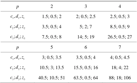
Table 9.1. Search intervals as functions of number of proc-essors p.
p 2 3 4
1, 1, 1
c d z 1.5; 0.5; 2 2; 0.5; 2.5 2.5; 0.5; 3
2; 2; 2
c d z 3.5; 0.5; 4 5; 2; 7 8.5; 0.5; 9
26.5; 0.5; 27
p
3; 3; 3
c d z 7.5; 0.5; 8 14; 5; 19
5 6 7
1, 1, 1
c d z 3; 0.5; 3.5 3.5; 0.5; 4 4; 0.5; 4.5
2; 2; 2
c d z 10.5; 3; 13. 5; 18; 4; 22
4
5 15.
6
0.5; 16
3; 3; 3
11. Inter
o
m
on
k
ort), i.e., PE(i) and PE(i + 1) are connected with MEM(i)
. (1 Then for large m(p) and m(1) holds that
ed probes in parallel and sequential modes are respectiv
-Pr cessor Co municati
Networ
1) All PEs are connected with
2) Two adjacent PEs share a memory unit (MEM, for a linear bus;
sh
and can read from it concurrently.
12. Speed-up and Efficiency of
Parallelization
Let bm p( ) 1 n bm p( ) and bm(1) 1 n bm(1) 2.1)
log
1 log
1m p u
p m u . (12.2) On the other hand, the numbers of requirely equal
2
1p
c n m p and c n1
2m
1 1. (12.3)Let’s define the speed-up of parallelization as
1
p p
s n c n c n . (12.4) Then (12.2) and (12.3) imply that
log
log 1p
u u p
s n .
If efficiency of parallelization is define
(12.5)
d as
:
p p
e n s n p, ( th
12.6) en
1
log 1
p p
e n c n pc n
p u
Since for the large number p of processors logu p
. (12.7)
2 1u p p ;
therefore for a large n
(see (A.15) and Table A.1 in Appendix) (12.8)
log 2 1
log p
log
p
1 5 2
s n p ; (12.9)
and finally
log
p
e n p p. (12.10)
13. Acknowledgements
Willard Miranker and J. Watson Research Ce nd Henryk Wozniakowski of Columbia University for
] J. L. Bentley and A. C.-C. Yao, “An Almost Optimal
Information Pro-
Vol. 5, No. 1, 1976, pp. 82-87.
I express my appreciation to
Shmuel Winograd of Thomas nter a
their comments and discussions. I also thank my former students Swetha Medicherla and Aleksey Koval for
sug-gestions that improved the style of this paper.
14. References
[1
Algorithm for Unbounded Searching,”
cessing Letters,
doi:10.1016/0020-0190(76)90071-5
[2] R. Beigel, “Unbounded Searching Algorithm,” SIAM Journal of Computing, Vol. 19, No. 3, 1990, pp. 522-537.
doi:10.1137/0219035
[3] E. M. Reingold and X. Shen, “More Nearly-Optimal Al-gorithms for Unbounded Searching, Part I, the Finite Case,” SIAM Journal of Computing, Vol. 20, No. 1, 1991, pp. 156-183. doi:10.1137/0220010
[4] E. M. Reingold and X. Shen, “More Nearly-Optimal Al-gorithms for Unbounded Searching, Part II, the Transfi-nite Case,” SIAM Journal of Computing, Vol. 20, No. 1, 1991, pp. 184-208. doi:10.1137/0220011
[5] A. S. Goldstein and E. M. Reingold, “A Fibonacci-Kraft Inequality and Discrete Unimodal Search,” SIAM Journal of Computing, Vol. 22, No. 4, 1993, pp. 751-777.
doi:10.1137/0222049
[6] A. S. Nemirovsky and D. B. Yudin, “Problems Complex-ity and Method Efficiency in Optimization,” W terscience, New York,
iley-In-1983.
er, “Minimax Optimization
, 1976, pp. [7] J. F. Traub and H. Wozniakowski, “A General Theory of
Optimal Algorithms,” Academic Press, San Diego, 1980. [8] J. H. Beamer and D. J. Wild
of Unimodal Function by Variable Block Search,” Man-agement Science, Vol. 16, 1970, pp. 629-641.
[9] D. Chasan and S. Gal, “On the Optimality of the Expo-nential Function for Some Minimax Problems,” SIAM Journal of Applied Mathematics, Vol. 30, No. 2
324-348. doi:10.1137/0130032
[10] J. C. Kiefer, “Sequential Minimax Search for a Maxi-mum,” Proceedings of American Mathematical Society, Vol. 4, No. 3, 1953, pp. 502-506.
doi:10.1090/S0002-9939-1953-0055639-3
[11] L. T. Oliver and D. J. Wilde, “Symmetric Sequential Minimax Search for a Maximum,
Vol. 2, No. 3, 1964, pp. 169-175.
” Fibonacci Quarterly,
ement Science, Vol. 12, No. 9, 1966, pp. [12] C. Witzgall, “Fibonacci Search with Arbitrary First
Evaluation,” Fibonacci Quaterly, Vol. 10, No. 2, 1972, pp. 113-134.
[13] M. Avriel and D. J. Wilde, “Optimal Search for a Maxi-mum with Sequences of Simultaneous Function Evalua-tions,” Manag
722-731. doi:10.1287/mnsc.12.9.722
[14] S. Gal and W. L. Miranker, “Optimal Sequential and Parallel Search for Finding a Root,” Journal of Combi-natorial Theory, Series A, Vol. 23, No. 1, 1977, pp. 1-14.
doi:10.1016/0097-3165(77)90074-7
No. 2, 1989, pp. 238-250.
[16] B. Verkhovsky, “Optimal Search Algorithm for Extrema of a Discrete Periodic Bimodal Function,” Journal of Complexity, Vol. 5,
doi:10.1016/0885-064X(89)90006-X
[17] B. Veroy (Verkhovsky), “Optimal Algorithm for Search of Extrema of a Bimodal Function,” Journal o
ity, Vol. 2, No. 4, 1986, pp. 323-332.
f
Complex-doi:10.1016/0885-064X(86)90010-5
[18] B. Veroy, “Optimal Search Algorithm for a Minimum of a Discrete Periodic Bimodal Func
Processing Letters, Vol. 29, No. 5, 19
tion,” Information
88, pp. 233-239.
doi:10.1016/0020-0190(88)90115-9
[19] S. Gal, “Sequential Minimax Search for a Maximum When Prior Information Is Available,” SIAM Journal Applied Mathematics, Vol. 21, No. 4,
of
1971, pp. 590-595.
doi:10.1137/0121063
[20] Yu. I. Neymark and R. T. Strongin, “Informative Ap-proach to a Problem of Search for an Extremum of a Function,” Technicheskaya Kibernetika, Vol. 1, 1966, pp
ubert, “A Sequential Method Seeking the Glob
a Global
Extre-. Hoffman and PExtre-. Wolfe, “Minimizing a Unimodal
eneralization of Fibonacci Search to
proxima-. 7-26.
[21] R. Horst and P. M. Pardalos, “Handbook of Global Opti-mization,” Kluwer Academic Publishers, Norwell, 1994.
[22] B. O. Sh al
Maximum of a Function,” SIAM Journal of Numerical Analysis,Vol. 3, No. 1, 1972, pp. 43-51.
[23] L. N. Timonov, “Search Algorithm for
mum,” Technicheskaya Kibernetika, Vol. 3, 1977, pp. 53- 60.
[24] A. J
Function of Two Integer Variables,” Mathematical pro-gramming, II. Mathematical Programming Studies, Vol. 25, 1985, pp. 76-87.
[25] A. I. Kuzovkin, “A G
the Multidimensional Case,” Èkonomka i Matematiches-kie Metody, Vol. 21, No. 4, 1968, pp. 931-940.
[26] J. C. Kiefer, “Optimal Sequential Search and Ap
tion Methods under Minimum Regularity Assumptions,”
SIAM Journal of Applied Mathematics, Vol. 5, 1957, pp. 105-136. doi:10.1137/0105009
[27] S. Gal, “A Discrete Search Game,” SIAM Journal of Ap-plied Mathematics, Vol. 27, No. 4, 1974, pp. 641-648.
doi:10.1137/0127054
[28] B. Verkhovsky, “Optimal Algorithm for Search of a
g Maximum of n-Modal Function on Infinite Interval,” In: D. Du and P. M. Pardalos, Eds., Minimax and Applica-tions, Academic Publisher, Kluwer, 1997, pp. 245-261. [29] B. Verkhovsky, “Parallel Minimax Unbounded Searchin
Appendix
A1. Complexity Analysis
A1.1. Basic Parameters
k
a interval added before k-th p-probe is computed;
k
g smaller interval on the k-th scanning state of the search;
k larger interval on the k-th scanning state of the
search; h
k interval of uncertainty eliminated from the search
after the k-th p-probe; w
k total interval added before the k-th p-probe is
per-formed; t
k total interval eliminated from the search as a result
of k p-probes. b
A1.2. Basic Relations: {oddp}
2
2 2 1
;
: ;
k k k k
k k k
k k k
a p h p g rh r g
r g h g
a h h
k
(A.1)
k and bk satisfy the following recursive relations for
all w
3 : k
1
; : ;
k k k k k k k
w a h g w h h (A.2)
1 1
:
k k
t h h r;
;
1kz. (A.3)
1 ; : 1.
k k k k k k
b b w b t h (A.4)
A1.3. Basic Relations: {evenp}
1 1
: ; : 1 ; : 2
: 1 ;
k
k k
k k
g z h r z w r
w r r z
(A.5)
1
1 1
: k k 1i
k i i i
b
w
r r z r (A.6) Let us consider for all k1 sequences hk, , vk kwith the following defining rules:
1 2: ;
k k k k k k
h v z h r h h
; (A.7) where1: 0; 0: 1; 1: 1; 0: 1 and 0 1
v v z . (A.8) (A.7) implies that
1 2
1 2: ; :
k k k k k k
v r v v r
.2
(A.9) It is easy to demonstrate by induction that for all
k
1 k .
k rv (A.10) Therefore
2 .
k k k
h v rv z (A.11)
If p = 1, then vk Fk, where all Fk are the
Fibo-nacci numbers.
Thus, all can be computed using the following formula:
k
v
;
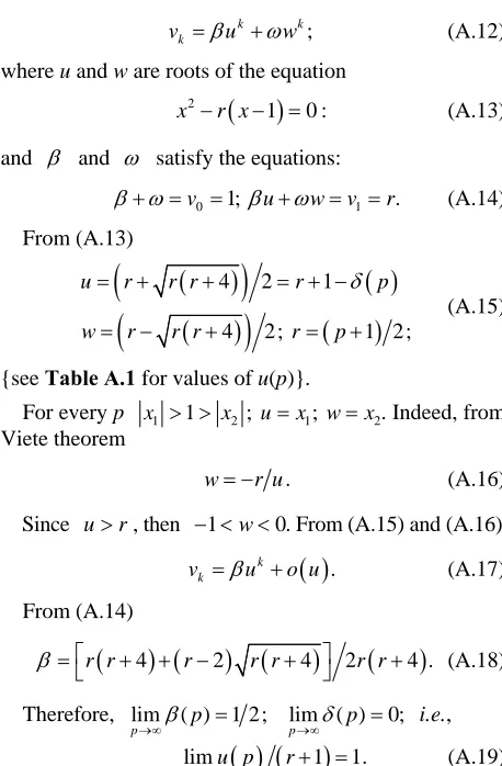
k k
v u wk (A.12) where u and w are roots of the equation
2
1 0
x r x : (A.13) and and satisfy the equations:
0 1; .
v u w v1 r
(A.14) From (A.13)
4 2 1
4 2; 1 2
u r r r r p
w r r r r p
;
(A.15)
{see Table A.1 for values of u(p)}.
For every p x1 1 x2 ; ux1; wx2. Indeed, from
Viete theorem
.
w r u (A.16) Since ur, then 1 w 0. From (A.15) and (A.16)
.k k
v u o u (A.17) From (A.14)
4
2
4
2
r r r r r r r
4 . (A.18)
Therefore, lim ( ) 1 2;
p p lim ( )p p 0; i.e.,
lim 1 1.
pu p r (A.19)
The latter limit in (A.19) means that for a large num-ber of processors u p
p3 2
.Examples A1: Table A.1 shows relationship between odd p and u(p).
A2. Maximal Intervals Analyzed after m
Parallel Probes
Proposition A.1: If s
vm11,vm1
, then m p-probes are required in the worst case to detect the maximizer on a final interval. [image:11.595.308.537.125.474.2]Proof is implied by (A.14) and (A.17). Proposition A.2: If p is odd, then
Table A.1. u(p) as function of odd number of processors p.
p p = 1 p = 5 p = 9