Modeling of Wave Propagation in General Dispersive Materials
with Efficient ADE-WLP-FDTD Method
Jun Quan1 and Wei-Jun Chen2, *
Abstract—Within the framework of the finite-difference time-domain (FDTD) and the weighted Laguerre polynomials (WLPs), we derive an effective update equation of the electromagnetic in the dispersive media by introducing the factorization-splitting (FS) schemes and auxiliary differential equation (ADE). As two examples, we employ a 2-D parallel plate waveguide loaded with two dispersive medium columns and a thin grapheme sheet to calculate the plane wave propagation by using the FS-ADE-WLP-FDTD method. Compared with the ADE-FDTD and the FS-ADE-WLP-FDTD methods, the results from our proposed method show its accuracy and efficiency for dispersive media simulation.
1. INTRODUCTION
The finite-difference time-domain (FDTD) method has been widely used for electromagnetic modeling due to its easy implementation [1]. However, because of Courant-Friedrich-Levy (CFL) stability constraint, the conventional FDTD is not very suitable for electromagnetic problems which involve fine grid division. To eliminate the limitation, some techniques, e.g., alternating-direction implicit (ADI) [2– 4] and locally one-dimensional (LOD) [5–7] methods, were proposed. Although these techniques can get more accurate simulation results and higher computational efficiency than the conventional FDTD, a large time step inevitably results in a large numerical dispersion error. Also, an unconditionally stable FDTD method using Laguerre polynomials has been proposed [8]. This marching-on-in-order scheme shows better efficiency than the conventional FDTD method when analyzing multi-scale structure.
Based on auxiliary differential equation (ADE), an unconditionally stable WLP-FDTD was proposed to simulate electromagnetic wave propagation in general dispersive materials [9]. The method introduces an ADE technique which establishes the relationship between the electric displacement vector and electric field intensity with a differential equation rather than a convolution integral. However, it leads to a huge sparse matrix equation, which is very challenging to solve. To solve the huge sparse matrix equation, an efficient algorithm is regularly used to implement the WLP-FDTD method [10], in which the huge sparse matrix equation is solved into a sub-steps procedure with a factorized-splitting scheme.
In this paper, a hybrid algorithm, known as factorization-splitting ADE-WLP- FDTD, is presented to improve its simulation performance. Based on the FS and ADE technique, our proposed algorithm only solves two tri-diagonal matrices and computes one explicit equation in 2-D problem. In comparison with the conventional implementation, less CPU runtime is spent. The accuracy and efficiency of the proposed method is verified by simulating electromagnetic wave propagation in a variety of dispersive media.
Received 19 November 2015, Accepted 11 January 2016, Scheduled 27 January 2016
* Corresponding author: Wei-Jun Chen (chenw [email protected]).
1 School of Physics Science and Technology, Lingnan Normal University, Zhanjiang 524048, China. 2School of Information Science
2. MATHEMATICAL FORMULATION
With lossless and dispersive media, the Maxwell’s equations read
∂D(r, t)
∂t = ∇ ×H(r, t)−J(r, t) (1) ∂H(r, t)
∂t = −
1
μ0∇ ×
E(r, t) (2)
where μ0 is the magnetic permeability of free space. The electric displacement vector D is related to
the electric field intensity E through the relative dielectric constantεr of the local tissue by
D(ω) =ε0εr(ω)E(ω) (3)
whereε0 is the electric permittivity in free space. In the frequency domain, εr can be written as [9, 11]
εr(ω) =ε∞
1 +
Nd
n
an
bn+jωcn−dnω2
(4)
where ε∞ is the infinite dielectric constant, ω the angular frequency, and an,bn,cn and dn are known
constants determined by the properties of the electric fieldsE(ω). Substituting Eq. (4) into Eq. (3), we get
D(ω) =ε0ε∞
E(ω) +
Nd
n
Sn(ω)
(5)
with
Sn(ω) = an
bn+jωcn−dnω2
E(ω) (6)
In terms of the transition relationshipjω→∂/∂t, Eqs. (5) and (6) can be casted into
D(r, t) =ε0ε∞
E(r, t) +
Nd
n=1
Sn(r, t)
(7)
bnSn(r, t) +cn∂
Sn(r, t)
∂t +dn
∂2Sn(r, t)
∂t2 =anE(r, t) (8)
Substituting Eq. (7) into Eq. (1) results in
∂E(r, t)
∂t +
Nd
n=1
∂Sn(r, t)
∂t =
1
ε0ε∞∇ ×
H(r, t)− 1
ε0ε∞
J(r, t) (9)
Using the weighted Laguerre basis functionsϕq(st), the field components can be expanded as [8]
{E,H,S(r, t)}=
∞
q=0
{Eq,Hq,Sq(r)}ϕq(st) (10)
wheres,q are time-scale factor and the order of Laguerre functions, respectively. For an arbitrary field componentU(r,t), for example, E,H,S(r,t), etc., the first and second derivatives of U(r,t) obey the following equations [8, 12], respectively,
∂U(r, t)
∂t = s ∞
q=0 ⎡
⎣0.5Uq(r) +
q−1
k=0,q>0
Uk(r)
⎤
⎦ϕq(st) (11)
∂2U(r, t)
∂t2 = s 2
∞
q=0 ⎡ ⎣Uq(r)
4 +
q−1
k=0,q>0
(q−k)Uk(r)
⎤
Inserting Eqs. (10)–(12) into Eqs. (2), (8) and (9), multiplying both sides by ϕp(st), and integrating
over st∈[0,∞), we have
Eq(r) +
Nd
n=1
Sqn(r) = 2
sε0ε∞∇ ×
Hq(r)− 2
sε0ε∞
Jq(r)−2
q−1
k=0,q>0
Ek(r)−2
Nd
n=1
q−1
k=0,q>0
Skn(r) (13)
Sqn(r) = 1
An
⎧ ⎨
⎩anEq(r)− q−1
k=0,q>0
cns+dns2(q−k)
Skn(r)
⎫ ⎬
⎭ (14)
Hq(r) = − 2
sμ0∇ ×
Eq(r)−2
q−1
k=0,q>0
Hk(r) (15)
where Jq(r) = Tf
0 J(r, t)ϕp(st)d(st), An = bn+ 0.5scn + 0.25s 2d
n, and Tf is a finite time interval.
Substituting Eq. (14) into Eq. (13), we may then write, instead of Eq. (13),
1 + Nd n=1 an An
Eq(r) = −2
q−1
k=0,q>0
Ek(r) +
Nd
n=1
san
An −
2
q−1
k=0,q>0
Skn(r)
+ 2
sε0ε∞∇ ×
Hq(r)− 2
sε0ε∞
Jq(r) + s
2d
An Nd
n=1
q−1
k=0,q>0
(q−k)Skn(r) (16)
Hence, Eqs. (15) and (16) can be written as a matrix equation form [8]. After obtaining the auxiliary differential variableS from Eq. (14), the electric fields are obtained by solving the matrix equation.
For the sake of simplicity, in the following sections we will employ a 2-D TEz case and single pole dispersive media (Nd= 1) to describe the procedures for deriving the FS-ADE-WLP-FDTD algorithm,
then thez-component of Hq(r) in (15) reads
Hzq(r) =
α,β α=β
σbDαEβq(r) +VHq−1(r) (17)
where b= 2/(μ0s), VHq−1(r) =−2 q−1
k=0,q>0Hzk(r). Dα =∂/∂α (α, β =x,y), is the first-order partial
differential operator, and α=x,σ =−1,α =y,σ = 1. The α-components ofEq(r) and Sq1(r) in Eqs. (14) and (16) are given by
Eαq(r) = AαDβHzq(r) +JEαq (r) +V q−1
Eα (r) +V q−1
Sα (r) (18)
S1qα(r) = 1/A1α
a1αEαq(r)−
q−1
k=0,q>0
c1αs+d1αs2(q−k)
S1kα(r)
(19)
whereAα, JEαq ,Vq−
1
Eα and Vq−
1
Sα are given by
Aα = A1α/[0.5ε0εα,∞s(a1α+A1α)] (20)
JEαq = −A1αJαq(r)/[0.5ε0εα,∞s(a1α+A1α)] (21)
withJαq describing the incident electric current excitation source along α axes.
VEαq−1(r) = −2A1α/(a1α+A1α) q−1
k=0,q>0
Eαk(r) (22)
VSαq−1(r) = (c1αs−2A1α)/(a1α+A1α) q−1
k=0,q>0
S1kα(r) +d1αs2
(a1α+A1α) q−1
k=0,q>0
(q−k)S1kα(r) (23)
Similar to the derivational procedure in [10], Eqs. (17)–(19) can be written as a matrix form
WqE = DHWqH +JqE +VqE−1+VqS−1 (24)
where WEq = [Exq Eyq]T,WqH = [Hzq], JqE = [JExq JEyq ]T,DH = [AxDy−AyDx]T,DE = [bDy −bDx],
VqE−1 =
VExq−1 VEyq−1 T
, VqS−1 =
VSxq−1 VSyq−1 T
. Combining Eqs. (24) and (25) leads to
WqE WqH
=
0 DH DE 0
WEq WHq
+
JqE 0
+
VqE−1 VqH−1
+
VSq−1 0
(26)
Let WqEH = WqE WHqT, JqEH = JqE 0, VqEH−1 =
VqE−1 VHq−1
and VqSH−1 =
VqS−1 0
T
, then Eq. (26) becomes
(I−A−B)WqEH=VEHq−1+VqSH−1+JqEH (27) with
A =
0 DHa DEa 0
=
0 0 0
0 0 −AyDx
0 −bDx 0
B =
0 DHb DEb 0
=
0 0
AxDy
0 0 0
bDy 0 0
Adding a perturbation termAB(WqEH−VqEH−1) to Eq. (27), we can obtain the factorized form
(I−A) (I−B)WqEH =ABVqEH−1+VqEH−1+VqSH−1+JqEH (28) Equation (28) can be computed into two sub-steps as following,
(I−A)W∗EHq = (I+B)VEHq−1+VqSH−1+JqEH (29) (I−B)WqEH = WEH∗q −BVqEH−1 (30)
where W∗EHq = WE∗q W∗HqT = E∗xq E∗yq H∗zqT. Using Eqs. (29) and (30) to solve Eq. (28) with some manipulations, we get
(I−DHaDEa)W∗Eq = (DHa+DHb)VHq−1+ (I+DHaDEb)VEq−1+VqS−1+JqE (31) (I−DHbDEb)WEq = (I+DHbDEa)WE∗q (32) WqH = DEbWqE+DEaW∗Eq+VHq−1 (33) Expanding Eqs. (31)–(33) leads to
Ex∗q = AxDyVHq−1+VExq−1+VSxq−1+JExq (34)
Eyq = Ey∗q (35)
(I−bAyD2x)Ey∗q = −AyDxVHq−1+VEyq−1−bAyDxDyVExq−1+VSyq−1+JEyq (36)
(I−bAxD2y)Exq = Ex∗q−bAxDyDxEy∗q (37)
Hzq = bDyExq−bDxEy∗q+Vq−
1
H (38)
whereD2α (α=x,y) is the second-order partial differential operator. Substituting Eqs. (34) and (35)
into Eqs. (36)–(38), we have
(I−bAyD2x)Eyq = −AyDxVHq−1+VEyq−1−bAyDxDyVExq−1+VSyq−1+JEyq (39)
(I−bAxD2y)Exq = AxDyVHq−1+Vq−
1
Ex +Vq−
1
Sx +JExq −bAxDyDxEyq (40)
Hzq = bDyExq−bDxEyq+Vq−
1
H (41)
the following form:
1 + bAy|i,j Δ¯x|i,j
1 Δx|i,j
+ 1 Δx|i−1,j
Eyq|i,j −ΔbAy|i+1,j
x|i,j Δ¯x|i,jE q
y|i+1,j −Δ bAy|i−1,j
x|i−1,jΔ¯x|i,jE q y|i−1,j
= Ay|i,j Δ¯x|i,j
VHq−1|i,j −VHq−1|i−1,j
+JEyq |i,j +VEyq−1|i,j +VSyq−1|i,j
− Ay|i,j b
Δy|i,j Δ¯x|i,j
VExq−1|i,j+1 −VExq−1|i,j −VExq−1|i−1,j+1 +VExq−1|i−1,j
(42)
1 + bAx|i,j Δ¯y|i,j
1 Δy|i,j−1
+ 1 Δy|i,j
Exq|i,j −ΔbAx|i,j+1
y|i,j Δ¯y|i,jE q
x|i,j+1 − bAx|i,j−1
Δy|i,j−1Δ¯y|i,jE q x|i,j−1
= −Ax|i,j Δ¯y|i,j
VHk|i,j −VHk|i,j−1
+VExq−1|i,j +JExq |i,j +VSxk |i,j
− Ax|i,j b
Δx|i,j Δ¯y|i,j E q
y|i+1,j −Eyq|i,j −Eyq|i,+1j−1 +Eyq|i,j−1 !
(43)
Hzq|i,j = Δ b
y|i,j
(Exq|i,j+1 −Exq|i,j)− Δb
x|i,j E q
y|i+1,j −Eyq|i,j
! −2
q−1
k=0,q>0
Hzk|i,j (44)
Comparing Eqs. (39) and (40) with [10], one can find that some parameters determined by dispersive media, Aα,α=x,y for example, are included.
3. NUMERICAL RESULTS
In order to validate the effectiveness of the FS-ADE-WLP-FDTD method, as the first example, we employ the wave transmission in a 2-D parallel plate waveguide with two dispersive medium columns, as depicted in Fig. 1. The staircase approximation is introduced to model dispersive medium columns. To improve the simulation precision, a fine grid division with cell size of 0.3 mm×0.3 mm is applied to the staircase region. The graded mesh is applied to rest computational regions, and the maximal cell is 10 mm×10 mm [9]. For simplicity, Mur’s 1st-order absorbing boundary conditions are used to truncate the computational area [8].
The first dispersive medium column is Debye model, in which the relative complex permittivity is given by
εr(ω) =ε∞+ε1 +s−jωτε∞ (45)
whereεs= 4.301, ε∞= 4.096 andτ = 2.294×10⁻⁹. The second dispersive medium column is Lorentz
model, in which the relative complex permittivity is given by
εr(ω) =ε∞+ (εs−ε∞) G1ω
2 1 ω2
1+ 2jδ1ω−ω2
(46)
x
y
ABC ABC
Jx 30 mm
100 mm
200 mm 1000 mm
100
m
m
P1 P2
where εs = 3, ε∞ = 1.5, ω1 = 2×10⁹rad/s, G1 = 0.4 and δ1 = 0.1ω1. A sinusoidally modulated
Gaussian pulse is used as a x-incident electric current profile
Jx(t) = exp
−
t−Tc
Td
2
sin 2πfc(t−Tc) (47)
where Td = 1/(2fc), Tc = 3Td and fc = 1 GHz. And we choose the time duration Tf = 11.71 ns, time
scaling factor s= 1.1902×10¹⁰ and order-marching step numberNL= 142.
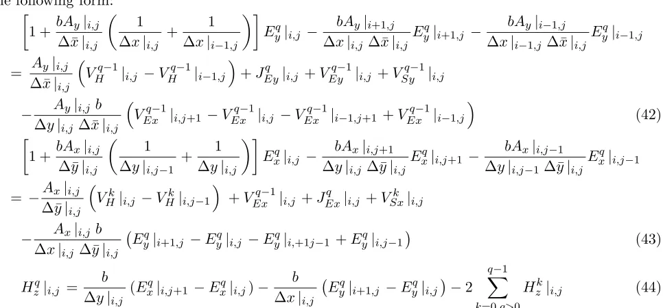
Figure 2 shows the calculated results given by the FS-ADE-WLP-FDTD, ADE-WLP-FDTD and ADE-FDTD. From their profiles, one can find that the FS-ADE-WLP-FDTD is accurate.
Table 1 shows the required computational resource and computing time for the numerical simulations. Compared with the ADE-WLP-FDTD and the ADE-FDTD, the FS-ADE-WLP-FDTD shows much improvement in computation efficiency. All calculations have been performed on an AMD Phenom II ×6 2.80 GHz machine with 8 GB RAM.
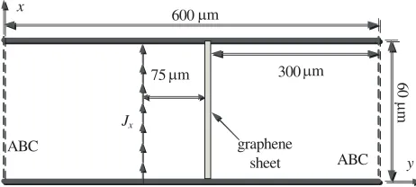
In the second example, the transmission coefficient of wave propagation in graphene sheets is calculated, as shown in Fig. 3. Here, we also choose x-polarization as the electric current excitation, andTc = 3Td,fc = 5000 GHz, the time durationTf = 1.5×10⁻¹²s, time scaling factors= 3.7699×10¹⁴
and order-marching step numberN = 150. Due to the structure with a thin layer in the computational domain, a fine grid division with the cell size of 1 nm×1500 nm is applied to the graphene layer. The graded mesh is applied to the rest computational regions, and the maximal cell is 1500 nm×1500 nm. In this example, the dispersive model of grapheme can be written as
εr(ω) =
1 + σ0/ε0
jω−τ ω2
(48)
with
σ0 = e 2τ k
BT
π2Δ
μc
kBT
+ 2 ln
e−kBTµc + 1
0 2 4 6 8 10 12
-1.0 -0.5 0.0 0.5
1.0 ADE-FDTD
ADE-WLP-FDTD FS-ADE-WLP-FDTD
Amplitude (a.u.)
0 2 4 6 8 10 12
-1.0 -0.5 0.0 0.5 1.0
Time (ns)
ADE-FDTD ADE-WLP-FDTD FS-ADE-WLP-FDTD
Time (ns)
Amplitude (a.u.)
(a) (b)
Figure 2. Transient electric fields of the x component (a) at P1 and (b)P2.
Table 1. Comparison of the computational efforts for the 2-D waveguide.
Method Δt(ps) Meshing size
y x
ABC
75 600
60
µ
m
graphene sheet
300
ABC
Jx
µm
µm
µm
Figure 3. Diagram of computational domain for WLP-FDTD analysis of graphene sheet.
0 2000 4000 6000 8000 10000
-8 -6 -4 -2 0
Theoretical ADE-FDTD ADE-WLP-FDTD FS-ADE-WLP-FDTD
Tr
ansmission coef
fi
cient (
d
B)
Frequency(GHz)
Figure 4. Transmission coefficient calcu-lated with the FS-ADE-WLP-FDTD, ADE-FDTDADE-WLP-FDTD and the theoretical so-lution.
where Δ, e, = h/2π, kB, T, τ and μc are the thickness of graphene sheets, electron charge,
reduced Plank’s constant, Boltzmann constant, temperature, scattering time and chemical potential, respectively [13]. Fig. 4 plots the numerical results of FS-WLP-FDTD, WLP-FDTD, ADE-FDTD and theory by setting Δ = 10 nm, μc = 0.5 eV, T = 300 K and τ = 0.5×10⁻¹²s. Compared
with the theoretical solution, the accuracy of the FS-ADE-WLP-FDTD method is verified.
Table 2 shows the comparison of the computing times among the three numerical methods. In Table 2, the FS-ADE-WLP-FDTD method also shows much more improvement in computation efficiency than the ADE-WLP-FDTD and ADE-FDTD methods.
Table 2. Comparison of the computational efforts for the graphene sheet.
Method Δt(fs) Meshing size Marching-on steps
Memory
(MB) CPU time(s) ADE-FDTD 1.67×10⁻³ 462×40 9×10⁵ 29 1722
ADE-WLP-FDTD 2.5 462×40 150 52 52
FS-ADE-WLP-FDTD 2.5 462×40 150 50 10
4. CONCLUSION
An ADE-WLP-FDTD method based on factorization splitting technique for general dispersive media is presented in this paper. Compared with the ADE-FDTD and ADE-WLP-FDTD, the FS-ADE-WLP-FDTD method can reduce the calculation burden. Two examples verify the accuracy and efficiency of the FS-ADE-WLP-FDTD method.
ACKNOWLEDGMENT
REFERENCES
1. Taflove, A. and S. C. Hagness,Computational Electrodynamics: The Finite-difference Time-domain Method, 2nd Edition, Artech House, Boston, MA, 2005.
2. Namiki, T., “A new FDTD algorithm based on alternating-direction implicit method,”IEEE Trans. Microw. Theory Tech. Vol. 7, No. 10, 2003–2007, Oct. 1999.
3. Kantartzis, N. V., T. T. Zygiridis, and T. D. Tsiboukis, “An unconditionally stable higher order ADI-FDTD technique for the dispersionless analysis of generalized 3-D EMC structures,” IEEE Trans. Magn., Vol. 40, No. 3, 1436–1439, Mar. 2004.
4. Kantartzis, N. V., D. L. Sounas, C. S. Antonopoulos, and T. D. Tsiboukis, “A wideband ADI-FDTD algorithm for the design of double negative metamaterial-based waveguides and antenna substrates,”IEEE Trans. Magn., Vol. 43, No. 4, 1329–1332, Apr. 2007.
5. Shibayama, J., M. Muraki, J. Yamauchi, and H. Nakano, “Efficient implicit FDTD algorithm based on locally one-dimensional scheme,”Electron. Lett., Vol. 41, No. 19, 1046–1047, Sep. 2005.
6. Rana, M. and A. Mohan, “Segmented-LOD-FDTD for electromagnetic propagation inside large complex tunnels,”IEEE Trans. Magn., Vol. 48, No. 2, 223–226, Feb. 2012.
7. Kantartzis, N. V., T. Ohtani, and Y. Kanai, “Accuracy-adjustable nonstandard LOD-FDTD schemes for the design of carbon nanotube interconnects and nanocomposite EMC shields,”IEEE Trans. Magn., Vol. 49, No. 5, 1821–1824, May 2013.
8. Chung, Y. S., T. K. Sarkar, B. H. Jung, and M. Salazar-Palma, “An unconditionally stable scheme for the finite-difference time-domain method,”IEEE Trans. Microw. Theory Tech., Vol. 51, No. 3, 697–704, Mar. 2003.
9. Chen, W.-J., W. Shao, and B.-Z. Wang, “ADE-Laguerre-FDTD method for wave propagation in general dispersive materials,”IEEE Microw. Wireless Compon. Lett., Vol. 23, No. 5, 228–230, May 2013.
10. Chen, Z., Y. T. Duan, Y. R. Zhang, and Y. Yi, “A new efficient algorithm for the unconditionally stable 2-D WLP-FDTD method,” IEEE Trans. Antennas Propag., Vol. 61, No. 7, 3712–3720, Jul. 2013.
11. Gandhi, O. P., B. Q. Gao, and J. Y. Chen, “A frequency-dependent finite-difference time-domain formulation for general dispersive media,” IEEE Trans. Microw. Theory Tech., Vol. 55, No. 4, 703–708, Apr. 2007.
12. Ha, M. and M. Swaminathan, “A Laguerre-FDTD formulation for frequency-dependent dispersive materials,” IEEE Microw. Wireless Compon. Lett., Vol. 21, No. 5, 225–227, May 2011.