Risk Measures and Capital Allocation

(1)

ABSTRACT

WANG, CHUN-JU. Risk Measures and Capital Allocation. (Under the direction of Peter Bloomfield.)

(2)

c

(3)

Risk Measures and Capital Allocation

by Chun-Ju Wang

A dissertation submitted to the Graduate Faculty of North Carolina State University

in partial fulfillment of the requirements for the Degree of

Doctor of Philosophy

Statistics

Raleigh, North Carolina 2010

APPROVED BY:

Sastry G. Pantula David A. Dickey

Min Kang Peter Bloomfield

(4)

DEDICATION

(5)

BIOGRAPHY

(6)

ACKNOWLEDGEMENTS

My profound appreciation goes to my adviser, Dr. Peter Bloomfield, who has been guiding my research with a lot of brilliant ideas, remarkable advice, and generous help. He has been always encouraging me with his gentle, kind, patient, and optimistic attitude not only for my research but also for my life. I am sincerely grateful that he would help me with going over the detail of my thesis even word by word so that I have been learning much writing skills from him. He has been very nice and definitely professional to work with so that I have been so lucky and very thankful to have him as my adviser.

I would like to thank Dr. Sastry G. Pantula, Dr. David A. Dickey, and Dr. Min Kang for serving as committee members of mine. Their insightful suggestions and comments have been making my work more complete, and I have learned a lot from their excellent lectures as well. I am thankful to Dr. Consuelo Arellano for giving me an opportunity of working with her on the project for Department of Plant Pathology at North Carolina State University. I would also like to thank Dr. Pam Arroway, Ms. Alison McCoy, and Mr. Adrian Blue for their hard work of assisting students in our department. My thanks also go to Dr. Huimei Liu, who advised my master thesis, Dr. Kang C. Jea, and Dr. Nan-Ping Yang, who are both from Fu Jen Catholic University, for their great advice and support on my career. I would like to thank Ms. Hsui-Chuan Wang, who is my High School English Teacher, because her excellent teaching inspired my passion for learning the second language, English.

(7)

TABLE OF CONTENTS

List of Tables . . . .viii

List of Figures . . . x

Chapter 1 Introduction . . . 1

1.1 General Introduction and Motivation . . . 1

1.2 Overview of Risk Measures and Capital Allocation . . . 2

1.2.1 Risk Measures . . . 2

1.2.2 Capital Allocation . . . 10

1.2.3 Summary of Contributions . . . 15

1.3 Overview of Thesis . . . 15

Chapter 2 Bias Adjustment Using Bootstrap Techniques for Estimating ES . 16 2.1 Introduction . . . 16

2.2 Bootstrap Techniques . . . 18

2.2.1 The Ordinary Bootstrap . . . 19

2.2.2 The Exact Bootstrap ofL-statistics . . . 21

2.2.3 Blockwise Bootstrap for Dependent Data . . . 22

2.3 Bias Adjustment for Simple ES Estimates . . . 23

2.3.1 For HS Estimates . . . 24

2.3.2 For GPD Estimates . . . 28

2.3.3 For MLE From Elliptical Distributions . . . 31

2.4 Bias Adjustment for Conditional ES Estimates of Time Series . . . 39

2.4.1 Conditional ES of ARMA Processes . . . 40

2.4.2 Conditional ES of GARCH Processes . . . 41

2.4.3 Conditional ES of ARMA-GARCH Processes . . . 46

2.5 Summary of Contributions . . . 47

Chapter 3 Evaluation of the Performance of Risk Models . . . 49

3.1 Model-based Criteria . . . 49

3.1.1 Existent Large Sample Properties of HS Estimates for ES . . . 50

3.1.2 Relative Accuracy Measures . . . 52

3.1.3 Simulation Study . . . 52

3.2 Data-based Criteria (Backtesting) . . . 75

(8)

3.2.2 Tests of Independence . . . 77

3.2.3 Joint Tests of Coverage and Independence . . . 82

3.2.4 The Bootstrap Test of Zero-mean Behaviour . . . 84

3.2.5 Simulation Study of Backtesting . . . 85

Chapter 4 Multivariate Framework for Estimating ES and ESC . . . 96

4.1 Introduction . . . 96

4.2 Methods Without a Volatility Filter . . . 96

4.2.1 Multivariate Version of Historical Simulation . . . 96

4.2.2 Multivariate Elliptical Distributions . . . 97

4.3 Conditional ES and ESC for MGARCH Processes . . . 99

4.3.1 Conditional ES and ESC for MGARCH-Gaussian Process . . . 100

4.3.2 Conditional ES and ESC for MGARCH-tProcesses . . . 101

4.3.3 Estimation Strategies . . . 102

4.4 Backtesting of ESC . . . 103

Chapter 5 Empirical Study . . . .104

5.1 Backtesting VaR and ES . . . 114

5.1.1 The Bootstrap Test of Zero-mean Behaviour . . . 114

5.1.2 Joint Tests of Coverage and Independence . . . 114

5.1.3 Test of Independence . . . 115

5.1.4 The Unconditional Coverage Test . . . 115

5.2 Backtesting ESC . . . 116

5.3 Conclusions . . . 116

Chapter 6 Conclusion and Future Topics . . . .117

6.1 Conclusion . . . 117

6.2 Future Topics . . . 118

6.2.1 Sequential Estimation of ESC for Higher Dimensional MGARCH . . . 118

6.2.2 Improvement of GPD Method With Optimal Threshold . . . 118

6.2.3 Other Estimation Methods for GARCH Models . . . 118

References. . . .119

Appendices . . . .124

(9)

Appendix B Proof of Proposition 1.10 . . . 127

B.1 To show (B.1) holds if either (B.2) or (B.3) is true . . . 127

B.2 To show either (B.2) or (B.3) is true, if (B.1) holds . . . 129

Appendix C Proof of Theorem 2.18 . . . 131

Appendix D Proof of Theorem 4.2 . . . 132

Appendix E Proof of Proposition 4.3 . . . 134

Appendix F Proof of Theorem 4.5 . . . 136

Appendix G Proof of Proposition 3.2 . . . 139

(10)

LIST OF TABLES

Table 3.1 Relative MSE of Original ES Estimates (Sample Size = 50) in % . . . 55 Table 3.2 Relative Accuracy Measures of Simple ES Estimates (Sample Size = 50) . 56 Table 3.3 Relative Accuracy Measures of ES Estimates for GARCH-N (Sample Size

= 50) . . . 57 Table 3.4 Relative Accuracy Measures of ES Estimates for EWMA (Sample Size =

50) . . . 58 Table 3.5 Relative Accuracy Measures of ES Estimates for GARCH-t (Sample Size

= 50) . . . 59 Table 3.6 Relative MSE of Original ES Estimates (Sample Size = 250) . . . 60 Table 3.7 Relative Accuracy Measures of Simple ES Estimates (Sample Size = 250) . 61 Table 3.8 Relative Accuracy Measures of ES Estimates for GARCH-N (Sample Size

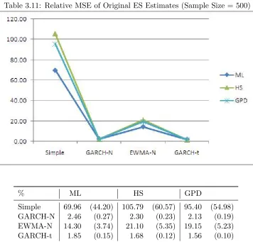
= 250) . . . 64 Table 3.11 Relative MSE of Original ES Estimates (Sample Size = 500) . . . 65 Table 3.12 Relative Accuracy Measures of Simple ES Estimates (Sample Size = 500) . 66 Table 3.13 Relative Accuracy Measures of ES Estimates for GARCH-N (Sample Size

= 500) . . . 69 Table 3.16 Relative MSE of Original ES Estimates (Sample Size = 1000) . . . 70 Table 3.17 Relative Accuracy Measures of Simple ES Estimates (Sample Size = 1000) 71 Table 3.18 Relative Accuracy Measures of ES Estimates for GARCH-N (Sample Size

= 1000) . . . 72 Table 3.19 Relative Accuracy Measures of ES Estimates for EWMA (Sample Size=1000) 73 Table 3.20 Relative Accuracy Measures of ES Estimates for GARCH-t (Sample Size

= 1000) . . . 74 Table 3.21 Contingency Table for Pearson’sχ2 Test of Independence . . . 79 Table 3.22 Sizes and Powers for Tests of Unconditional Coverage (Pseudo Estimate

(11)

Table 3.23 Sizes and Powers for Tests of Unconditional Coverage (GM Estimate of VaR) . . . 88 Table 3.24 Sizes for Tests of Independence (Pseudo Estimate of VaR) . . . 90 Table 3.25 Powers for Tests of Independence (GM Estimate of VaR) . . . 91 Table 3.26 Sizes and Powers for Joint Tests of Coverage and Independence (Pseudo

Estimate of VaR) . . . 93 Table 3.27 Powers for Joint Tests of Coverage and Independence (GM Estimate of VaR) 94

(12)

LIST OF FIGURES

Figure 2.1 Real World vs. Bootstrap World . . . 18

Figure 3.1 Sizes and Powers for Tests of Unconditional Coverage (Pseudo Estimate of VaR) . . . 87

Figure 3.2 Sizes and Powers for Tests of Unconditional Coverage (GM Estimate of VaR) . . . 88

Figure 3.3 Sizes for Tests of Independence (Pseudo Estimate of VaR) . . . 90

Figure 3.4 Powers for Tests of Independence (GM Estimate of VaR) . . . 91

Figure 3.5 Sizes and Powers for Joint Tests of Coverage and Independence (Pseudo Estimate of VaR) . . . 93

Figure 3.6 Powers for Joint Tests of Coverage and Independence (GM Estimate of VaR) . . . 94

Figure 5.1 Structure of The Empirical Study . . . 105

Figure 5.2 Plot of Daily Values . . . 107

Figure 5.3 Plot of Daily Losses . . . 108

Figure 5.4 Plot of Russell 1000 Index and the Predicted ES . . . 109

Figure 5.5 Plot of Russell 2000 Index and the Predicted ES . . . 110

Figure 5.6 Plot of Aggregate Index and the Predicted ES . . . 111

Figure 5.7 Plot of Russell 1000 Index and the Predicted ESC . . . 112

(13)

Chapter 1

Introduction

1.1 General Introduction and Motivation

The development of financial risk management has been of active interest to regulators, re-searchers, specialists associated with the field, and financial institutions themselves. Much of it originates from the need to quantify, control, and report the risks that a financial institution faces, in the sense of the essential level of uncertainty about the future, comprised of market, credit, liquidity, operational, and systemic risks. The essence is that the amount of capital a financial institution needs should be determined as a buffer to absorb unexpected losses from those risks that could otherwise lead the financial institution to insolvency. Such capital is then called risk capital, and the determination of it has become prominent, since a financial institution is required to hold appropriate risk capital for keeping the possibility of insolvency acceptably low; meanwhile it must still be competitive in the capital market. At the inter-national level, regulators such as the Interinter-national Association of Insurance Supervisors and the Basel Committee on Banking Supervision (BCBS), to name but two, make many efforts to develop a set of rules for the world’s accounting, banking, or insurance systems in order to provide a safer trading environment.

(14)

nature of the application and the amount of information available, the problem becomes how to estimate the measure of risk and the allocated capital based on the specified risk measure. In order to choose a more suitable estimator, evaluation of the performance of estimates calculated by different methods is investigated as well. For comprehensive reviews of risk measurement, please refer to McNeil et al. (2005) and Dowd (2005b). The former, by McNeil et al. (2005), provides core concepts, techniques and tools of quantitative modeling issues for financial risk management. It also covers the issue of capital allocation. The latter, Dowd (2005b), addresses how to measure the market risk, including estimation of VaR and ES.

This research will first review risk measures and risk capital allocation, along with the im-portant property of coherency, and the relationships between different coherent risk measures. Secondly, relative accuracy measures will be used as model-based criteria to study whether or not bias adjustment by various bootstrap techniques could improve estimates of the ex-pected shortfall (ES) as a risk measure. Thirdly, tests for backtesting ES will be investigated as data-based criteria of evaluating ES estimates. Fourthly, based on multivariate framework, estimation of (conditional) ES and ES risk contributions (ESC), as a principle of capital allo-cation, will be studied. Finally, an empirical study of estimating ES and ESC with backtesting will be carried out for historical data from Russell Indices.

1.2 Overview of Risk Measures and Capital Allocation

1.2.1 Risk Measures

Interest has been increasing in the subject of how to describe the many and various risks a financial institution faces or a portfolio is exposed to. The measurement of risk gives us a quantitative tool to tell how risky the business of a financial institution (or a portfolio) is. A risk measure, quantitative measurement of risk, is a number which is designed to evaluate the magnitude of risk and capture the primary properties of the risk.

Coherent Risk Measures

Proposed risk measures are judged by whether they satisfy specific desirable properties of risk measures, collected as the axioms of coherence, a concept developed by Artzner et al. (1999). Definition 1.1. (Axioms of Coherent Risk Measure; Artzner et al. (1999)). Suppose that G is the set of all real-valued measurable functions on the sample space Ωof outcomes. A risk measure ρ:G →_R∪ {+∞}is said to be coherent if it satisfies the following four axioms:

1. Subadditivity: For allX ∈ G, Y ∈ G,

(15)

2. Monotonicity: For allX ∈ G andY ∈ G such that X≤Y, ρ(X)≥ρ(Y)

3. Positive Homogeneity: For any number λ≥0 andX ∈ G, ρ(λX) =λρ(X)

4. Translation Invariance: For any constant k∈_R, ρ(X+kr) =ρ(X)−k

where r is the price of a riskless instrument at the end of the holding period with price 1 today.

Subadditivity is necessary to incorporate the property that diversification of portfolios has a positive impact, which means that combining two portfolios does not create extra risk. Mono-tonicity says that if a portfolio Y is always worth more than X, then Y should not be riskier than X. Positive homogeneity is a limit case of subadditivity, meaning what happens when no diversification occurs. It also has the interpretation that the risk measure is independent of scale changes (e.g. currency changes) in the unit in which the risk is measured. However, it is debatable, since the risk in the position may become unacceptable in case r is large enough, although it is innocuous for moderate values of r. Translation invariance is a natural require-ment and also known asRisk-free condition. It represents that adding a sure amount of money decreases the measurement of risk by the same amount. Notice that no probability measure on Ω has been involved.

Note that no probability spaces are involved in the axioms of coherent risk measures (Def-inition 1.1). (Artzner et al., 1999) not only introduced the def(Def-inition of coherent risk measure but also generalized the computation of SPAN margin system (SPAN, 1995), developed by the Chicago Merchantile Exchange, to scenario-based risk measures defined below. It provided a general way to construct a coherent risk measure by using a family of probability measures and quantifying risks as the worst-case expected loss.

The definition of scenario-based risk measures (SBRM) is given as follows.

Definition 1.2. (Scenario-based Risk Measures). The scenario-based risk measure defined by a non-empty set P of probability measures or generalized scenarios on the space Ω for a random variable X is the function ρ_P on G, the set of all real-valued functions on Ω, defined by

ρ_P(X) = sup

P∈P

(16)

Initially there is no particular probability measure on Ω. Artzner et al. (1999) discussed the relationship between coherence and scenario-based risk measures, along with the following two propositions.

Proposition 1.3. (Artzner et al. (1999)). Given the non-empty set P of probability mea-sures, or generalized scenarios, on the set Ω of states of the world, the risk measure ρ_P of Definition 1.2 is a coherent risk measure. It satisfies the relevant axioms if and only if the union of the supports of the probabilities P ∈ P is equal to the set Ω.

Proposition 1.4. (Artzner et al. (1999)). A risk measure ρ is coherent if and only if there exists a family P of probability measures on the set of states of nature, such that

ρ_P(X) = sup

P∈P

EP(−X).

Proofs of Propositions 1.3 and 1.4 are provided in Artzner et al. (1999) as well.

Furthermore, Delbaen (2002) extended Definition 1.1 to coherent risk measures on general probability spaces by characterising closed convex sets of probability measures which satisfy the property that every random variable is integrable for at least one probability measure in this set. Please refer to his context for more reference and details.

Value at Risk

The notion of Value-at-Risk or VaR was introduced by Morgan (1995) as a risk management tool, and made a major breakthrough in the evolution of modern risk measures. VaR has been extensively applied to determine the required risk capital which a financial institution should hold to cover its worst case loss. VaR has been employed by regulatory bodies such as the Basel Committee on Bank Supervision (BCBS) which published the 1996 Amendment

(BCBS, 1996, Amendment to the capital accord to incorporate market risks). VaR is extended straightforwardly frompossible maximum lossaspossible maximum loss which is not exceeded within a given confidence level over a given holding period (McNeil et al., 2005). Suppose that

Xdenotes the profit and loss (P&L) of either the business of the underlying financial institution or the specified portfolio, which takes the risk. In other words, X is the change in the value of the business of the underlying financial institution or of the specified portfolio between the date of calculation and a future date. Given the probability distribution ofX, the VaR at the confidence level α is the smallest number x such that the probability that the loss will exceed

(17)

Definition 1.5. (Value at Risk; McNeil et al. (2005)). VaR at the confidence level α is defined as

VaRα(X) = inf{x∈R:P(−X > x)≤1−α}.

See McNeil et al. (2005) or Acerbi and Tasche (2002) for more discussion. This definition of VaR presumes that X(ω) ∈ _R for all ω ∈ Ω where Ω is the sample space of outcomes. Furthermore,

VaRα(X) =qα(−X)

(Tasche, 2002b) where qα(Y) denotes the lower α-th quantile of Y1. In the case where X is continuous with a strictly positive density function, the cumulative distribution function (cdf) of X is a continuous and strictly monotonic distribution function and VaR(X) is the unique solution for x of the equation

P(−X≤x) =α.

Alternatively, VaR can be interpreted as the minimum loss incurred in the (1−α)% worst cases of the P&L. In practice, the time horizon used is usually the one day or ten days period and the value for levelα is quite high and close to 1, typically 95% or 99%. Despite the widespread use of VaR as a standard risk measure among practitioners in the financial market, it has many deficiencies and inconsistencies when applied in real life applications. Particularly, it is heavily criticized for failing to satisfy the subadditivity axiom of coherent risk measures defined in Definition 1.1 and therefore fails to encourage diversification, while clearly satisfying the other three axioms: monotonicity, positive homogeneity, and translation invariance (Artzner et al., 1999, l.c.). Comprehensive discussions on VaR can be found in Jorion (2001) and Holton (2003).

Expected Shortfall

An alternative to VaR is expected shortfall, of which definition is given in 1.6. Discussion on VaR and Tail VaR as risk measures can be found in Overbeck (2000). The most popular and widely-accepted risk measure, expected shortfall, has attracted a lot of attention in current development of risk measures. Under proper conditions, it is also known as tail value at risk, Tail VaR (Artzner et al. (1999)) or CTE, conditional tail expectation (Wirch and Hardy (1999)). Differences between most definitions of expected shortfall were discussed in Tasche (2002a) and Tasche (2002b). The expected shortfall is preferred as a standard risk measure presently, since it satisfies the axioms of coherence proposed by Artzner et al. (1999). Expected shortfall can be generally represented as an average of excess losses or mean shortfall and formally defined at the confidence level α in Definition 1.6.

1_q

(18)

Definition 1.6. (Expected Shortfall; Tasche (2002b)). Suppose that (Ω,A, P) is a prob-ability space and a fixed confidence level α ∈ (0,1) close to 1. Define X− as max(0,−X). Consider a real random variable (r.v.) X on (Ω,A, P) with E(X−) < ∞ and the indicator functionIA2. Then

ESα(X) =−(1−α)−1{E[X·I_{−_X_≥_VaR_α₍_X₎_}] + VaRα(X)·(α−P[−X <VaRα(X)])} (1.2) is called Expected Shortfall (ES). The most popular way to define ES (Tasche, 2002b; McNeil et al., 2005)is that

ESα(X) =

1 1−α

Z 1

α

VaRu(X)du, (1.3)

which is equivalent to (1.2).

Equation (1.2) was first introduced in Acerbi et al.. The representation of ES in (1.3) was first established by Wirch and Hardy (1999) for X ≥ 0 and given by Bertsimas et al. (2000) for continuous distributions. The representation in (1.3) is easy to be described as theaverage of the 100(1−α)% worst losses of X. It follows that ESα(X) ≥ VaRα. The proof of the

equivalence of (1.2) and (1.3) can be found in Acerbi and Tasche (2002, Proposition 3.2). The proof of coherency of ES can be found in Acerbi and Tasche (2002). Besides, there are two alternative ways to show the coherency of ES and the detail will be summarized in Section 1.2.1 later. One of them takes advantage of the connection between ES and spectral risk measures, which will be introduced in the next section. The other way takes advantage of the connection between ES and scenario-based risk measures, described in Proposition 1.7 below.

Proposition 1.7. Suppose that given a model with distribution P and the probability space

(Ω,A, P). Consider the family Q of those measures which are boundedly stressed versions of P, in the form of

Q=

Q: dQ

dP ≤k

, (1.4)

for some constant k >1. Afterwards, by taking k= 1/(1−α), the scenario-based risk measure ρ_Q(X) = sup_Q_∈_QEQ(−X) turns out to be

1 1−α

Z 1

α

VaRu(X)du,

which is exactly the ES with respect to P at confidence level α.

2_I

A=

(19)

The discussion and proof of Proposition 1.7 can be found in Delbaen (2002). Proposition 1.7 indicates that for ES as a risk measure, there exists a family of probability measures on the set of states of nature so that ES is coherent by Proposition 1.4. Hence this gives an alternative way to show coherency of ES.

The following introduces conditional tail expectation (CTE) or namely tail conditional ex-pectation (TCE), which is closely related to ES but does not coincide in general. CTE has received extensive attention due to its identity to ES under suitable conditions such as the continuity of the distribution functionFX(x).

Definition 1.8. (Conditional Tail Expectation (CTE)). The conditional tail expectation for a real random variableX at confidence level α is given by

CTEα(X) = E[−X|X≤ −VaRα(X)]. (1.5)

Generally CTE may not be coherent due to violation of subadditivity, as mentioned by Acerbi and Tasche (2002, Example 5.4) and stated by Delbaen (2002, Theorem 6.10).

The relationship between ES and CTE is synthesized as follows. Manifestly ES is continuous inαin (1.3) while it is not in (1.2). This is a distinguishing feature of ES which CTE and VaR do not possess.

Proposition 1.9. Generally, CTEα(X)≤ESα(X).

Proposition 1.10. CTEα(X) = ESα(X) if and only if one of the following conditions holds. 1. Pr[X≤ −VaRα(X)] = 1−α.

2. Pr[X <−VaRα(X)] = 0.

Although similar statements and proofs of Proposition 1.9 and 1.10 can be found in Acerbi and Tasche (2002, Corollary 5.2 and 5.3, respectively), herein more precise and direct proofs of them are provided in Appendix A and Appendix B, respectively. It is observed from the proofs that a first sufficient condition for CTE and ES to coincide is the continuity of the distribution of X.

(20)

Kim (2007) derived the CTE formula for exponential family. Furthermore, Jalal and Rockinger (2006) investigated the consequences for VaR and ES of using a GARCH filter on various mis-specified process. McNeil et al. (2005) provides comprehensive formulas of conditional ES for both univariate and multivariate GARCH models. Furman and Landsman (2008) derived analytical CTE formulas for multivariate Poisson distributions, which are not continuous, and hence take notice of that its CTE does not equal to its ES.

Spectral Risk Measures

Employing ES as the basic building block, Acerbi (2002) proposed spectral risk measures by generating a new class of risk measures based on ES. It turns out that spectral risk measures take explicit account of a user’s degree of subjective risk aversion which neither VaR nor ES does. Please refer to Acerbi (2002) for more details therein. An additional preliminary is needed before introducing it. Let a norm spaceL1([0,1]) be a space, where every element is represented by a class of functions which differ at most on a subset of [0,1] of zero measure. The norm in this space is defined by

||φ||= Z 1

0

|φ(p)|dp.

The Spectral Risk Measure (SRM) is defined in Definition 1.11.

Definition 1.11. (Risk Aversion Function and Spectral Risk Measure; Acerbi (2002)). The class of Spectral Risk Measure Mφ of a r.v. X, generated by an admissible risk spectrum φ∈ L1([0,1]), is given by all measures of the type:

Mφ(X) = Z 1

0

VaRp(X)φ(p)dp, (1.6)

where φ: [0,1]→ _R is then called the Risk Aversion Function of Mφ, satisfying the following conditions.

• Non-negativity

φ(p)≥0 for allp∈[0,1] • Normalization

||φ||= Z 1

0

|φ(p)|dp= Z 1

0

φ(p)dp= 1

• Monotonicity (non-increasingness)

(21)

i.e.

φ(1)(p)≤0

provided that the first derivative of φexists.

Theφfunction is nothing but a weight function in (1.6) which averages the possible outcomes of the random variable X. Besides, different representative functions φ1, φ2 (||φ1−φ2|| = 0) of the same element φ∈ L1([0,1]) will actually define the same measure Mφ. Furthermore, as stated in Theorem 1.12 belowMφdefined above is coherent if and only if its risk spectrumφis

admissible, which means it satisfies all the conditions therein.

Theorem 1.12. (Acerbi (2002)[Theorem 4.1]) A spectral risk measure is a coherent risk measure if and only if the risk spectrum, which generates it, is admissible.3

TheMonotonicity (non-increasingness)property provides an intuitive insight of the concept of coherence. As a matter of fact, the necessary and sufficient condition for a SRM to be coherent, which states that its risk spectrum φ should be admissible, gives a reasonable rule:

a risk measure is coherent if it assigns larger weights to worse cases. For example, the risk spectra for VaR and ES can be written in the form of

δ(p−α) and

1

1−αI{α≤p≤1},

respectively, where δ(x) is the Dirac Delta function defined by

Z b

a

f(x)δ(x−c)dx=f(c), ∀c∈(a, b).

As a result, it is easy to see that VaR is not coherent, since its risk spectrum is not admissible. Similarly, ES is coherent, since its risk spectrum is admissible.

By the above proposition, for a spectral risk measureMφ(X) with admissible risk spectrum, there exists a family P of probability measures on the set of states of nature, such that

Mφ(X) =ρ_P(X),

where ρ_P(X) is the scenario-based risk measure defined by P. However, it remains an open question of how to characterize the existing familyP of probability measures forMφ(X). Since

ES is a special case of scenario-based risk measures and of spectral risk measures, the next

(22)

tion will discuss more on coherency and ES by exploiting the connection between ES, scenario-based risk measures and spectral risk measures, and the fact that scenario-scenario-based risk measures and spectral risk measures are all coherent.

Supplementary

It has been shown that ES satisfies all properties defined in Definition 1.1 and hence is coherent. By incorporating previous results in the foregoing sections, it is also easy to show the coherency of ES in two alternative ways as follows.

1. Proposition 1.7 indicates that for ES as a risk measurere, there exists a family P of probability measures on the set of states of nature and hence ES is a scenario-based risk measure defined by P. Thus ES is coherent by Proposition 1.4.

2. We know that ES is a spectral risk measure generated by the admissible risk spectrum

φ(p) = ₁₋1_αI{α≤p≤1}. Therefore, ES is coherent by Theorem 1.12.

1.2.2 Capital Allocation

The capital allocation problem is that once the total risk capital for a multi-unit financial insti-tution (or a combination of different portfolios) is computed based on a specific risk measure, the risk capital must be allocated back to each business unit (or portfolio) in a consistent way which should recognize the benefit of diversification. Different allocation methods are avail-able; however, only some of them satisfy the nice properties which have economical meanings, while others do not. Those desirable properties were proposed as axioms of coherent alloca-tion(Denault, 2001) and fair allocation(Kim, 2007) (adapted from Valdez and Chernih (2003) which extended Wang’s4 idea to the elliptical distribution class for capital allocation problem), respectively. They will be discussed in the next section.

Axioms of Allocation Principles

Consider an investor who can invest in a fixed set ofdindividual investment possibilities with P&L denoted by the random variablesX1, X2, . . . , Xd. LetC =ρ(S) andCi denote the overall risk capital determined by a particular risk measure, and the allocation ofCto thei-th portfolio, respectively. The P&L of the actual portfolio is of courseS =Pd

i=1Xi. An allocation principle

is a function that maps allocation problems associated with a specified risk measure into a unique allocation. Next section will cover axioms of coherent allocation principle and those of fair allocation principle.

4

(23)

Definition 1.13. (Axioms of Coherent Allocation; Denault (2001)). An allocation principle is coherent if it satisfies the following axioms:

1. Full allocation: The allocated risk capitals add up to the total risk capital.

ρ(S) =

d

X

i=1

Ci (1.7)

2. No undercut: For any subset M of {1,2, . . . , d},

X

k∈M

Ck≤ X

k∈M

ρ(Xk) (1.8)

3. Symmetry: If by joining any subset M of {1,2, . . . , d}\{i, j}, portfolios i and j have identical contribution to the risk capital, then Ci=Cj.

4. Riskless allocation: If the dth portfolio is a riskless instrument, then

Cd=ρ(αr) =−α

where r is the price, at the end of the holding period, of a reference riskless instrument whose price is 1 at the beginning of the period.

Full allocation means that the overall risk capital is fully allocated back to the individual portfolio positions. No undercut addresses the diversification effect as a reward. That is, an investor holding the portfolio could benefit from the diversification of combination of portfolios. Symmetry ensures that the allocation of a portfolio depends only on its contribution to risk and nothing else. Riskless allocation means that when all other things are equal, a portfolio that increases its cash position results in decrease of its allocated capital by the same amount. Definition 1.14. (Axioms of Fair Allocation). An allocation principle is fair if it satisfies the following axioms:

1. Full allocation: The allocated risk capitals add up to the total risk capital.

ρ(X) =

d

X

i=1

Ci (1.9)

2. No undercut: For any subset M of {1,2, . . . , d},

X

k∈M

Ck≤ X

k∈M

(24)

3. Symmetry: If by joining any subset M of {1,2, . . . , d}\{i, j}, portfolios i and j have identical contribution to the risk capital, then Ci=Cj.

4. Consistency: For any subset M of {1,2, . . . , d} with |M| = m, let X∗ = P

i∈MXi and Xd−m = (Xj1, . . . , Xjm)

0 _{for all} _j

k ∈ {1,2, . . . , d}\M, where k = 1, . . . , d− m. Then the new hierarchical structure of thedindividual portfolios becomesX∗,X0_d₋_m as a combination of individual d−m+ 1 portfolios. Let C₁∗ denote the allocated capital of the portfolio X∗ as an individual one, computed on X∗,X0_d₋_m. Afterward

X

i∈M

Ci =C1∗. (1.11)

Obviously, the definition of fair allocation adopts the first three axioms of coherent allocation but replaces the last one, riskless allocation, by consistency. Consistency ensures that the allocation of an individual portfolio cannot depend on the level at which allocation is calculated. For instance, consider a company consisting of multiple units of business at the top level and sub-units of business at lower level. According to the consistency axiom, the capital allocation for a unit of business at the top level must be identical whether the allocation of its sub-units has been directly computed to the company or indirectly first to the top level and later aggregated for the company. In sum, the allocated capital for one unit of business should be independent of the hierarchical structure of the company.

Euler Capital Allocation Principle

Consider the random variablesX1, X2, . . . , Xdon a common probability space (Ω,A, P) as the

P&L for d individual investment possibilities. Let C = ρ(S) and Ci denote the total risk

capital determined by a specified risk measure, and the allocation of C to the i-th portfolio, respectively. Furthermore, consider a set U ⊂_Rd\ {(0, . . . ,0)} of portfolio weights and define

S(u) =Pd

i=1uiXi foru= (u1, . . . , ud)∈U. The total P&L of the actual portfolio is of course S(I) =Pd

i=1Xi. Letρdenote some risk measure defined on a setMwhich contains the random

variables {S(u) :u∈U}. Then introduce the associated risk-measure function fρ:U →_R

fρ(u) =ρ(S(u)). (1.12)

Thusfρ(u) is the required total risk capital for a positionuin the set of investment possibilities. Definition 1.15. Let fρ be a risk-measure function on some set U ⊂ Rd\ {(0, . . . ,0)} such that (1, . . . ,1) ∈ U. A mapping πfρ : U → R

(25)

associated with fρ, if

d

X

i=1

uiπi=fρ(u), (1.13)

where πi represents the i-th element of πfρ(u).

This definition interprets that the i-th element ofπfρ(u) gives the amount of capital to one

unit of Xi, when the overall position has P&L S(u). The amount of capital allocated to the

positionuiXi isuiπi and the equality (1.13) is simply the full allocation property.

Definition 1.16. (Positive Homogeneity). A function f :U ⊂Rd → R is called homoge-neous of degree kif for any γ >0 and u∈U with γu∈U the following equation holds:

f(γu) =γkf(u)

where k is a positive integer.

Note that positive homogeneity in McNeil et al. (2005) is in fact positive homogeneity of degree 1. If the risk measure ρ is homogeneous of degree k, then the risk-measure function fρ

coresponding by (1.12) to ρ is homogeneous of degree k. In the case of continuously differen-tiablility, homogeneous functions can be characterized by Euler’s theorem as follows.

Theorem 1.17. (Euler’s theorem). Let U ⊂ _Rd _{be an open set and} _f _: _U _→

R be a continuously differentiable function. Thenf is homogeneous of degreekif and only if it satisfies

kf(u) =

d

X

i=1

ui∂f ∂ui(u).

Therefore, by Euler’s theorem, the risk-measure function fρ(u) satisfies

fρ(u) = d

X

i=1

ui ∂fρ(u)

∂ui

(u) (1.14)

if and only if it is homogeneous of degree 1. Hence comparison of (1.13) and (1.14) gives Euler capital allocation principle defined in Definition 1.18.

Definition 1.18. (Euler capital allocation principle). Suppose that a risk-measure func-tion fρ is positive homogeneous of degree 1 on some set U ⊂ Rd \ {(0, . . . ,0)} such that

(1, . . . ,1) ∈ U. Assume that f is continuously differentiable; then the per-unit Euler capital allocation principle associated with fρ is the mapping

πfρ:U →R

d_, _πf

ρ(u) =

∂fρ ∂u1

(u),∂fρ ∂u2

(u), . . . ,∂fρ ∂ud

(u)

(26)

The Euler capital allocation principle is also called allocation by the gradientsand satisfies the full allocation property, which means that the overall risk capitalfρ(u) is fully allocated back to the individual portfolio positions. Tasche (2007, 2008) showed that the risk contributions to some risk measure ρ with continuously differentiable fρ are uniquely determined by Euler

capital allocation withu= (1, . . . ,1) if and only iffρis positive homogeneous of degree 1. Then those risk contributions, uniquely determined by the Euler capital allocation with u= (1, . . . , 1), are called Euler contributions. A comprehensive description of the Euler capital allocation principle and more reference of it can be found in Tasche (2007, 2008). The Euler allocation principle was also justified by other authors by different approaches. Denault (2001) derived the Euler allocation principle by game theory and it was regarded asAumann-Shapley per-unit allocationfor homogeneous risk measures of degree one. That is, the Aumann-Shapley per-unit allocation is equivalent to the Euler capital allocation. Additionally, it is shown as a coherent allocation of risk capital as well in his paper.

In the continuous case, by employing the risk-measure function

ρESα(u) = (1−α)

−1 Z 1

α

ρVaRp(u)dp

where ρVaRp(u) = VaRp(u), the Euler risk contributions corresponding to the risk measure ES

is called expected shortfall contributions (ESC) and given by

ESCα(Xk) =−E[Xk|S ≤ −VaRα(S)], k= 1, . . . , n. (1.16)

(27)

1.2.3 Summary of Contributions • Comprehensive literature review

• Direct and clear statements in Proposition 1.9 and 1.10 and their proofs

1.3 Overview of Thesis

All studies hereafter are started from the losses as the data, which is merely the negative value of the P&L, for convenience. In other words, suppose that a random sampleS = (S1, . . . , Sn)0

of potential total losses such that Si = Pm

j=1Xi,j, i = 1,2, . . . , n. The formulas of expected shortfall and its contributions are then given by

ESα(S) =

1 1−α

Z 1

α

VaRu(S)du (1.17)

and

ESCα(Xk) = E[Xk|S ≥VaRα(S)]; k= 1, . . . , m, (1.18)

(28)

Chapter 2

Bias Adjustment Using Bootstrap

Techniques for Estimating ES

2.1 Introduction

Dowd (2005a) and Hardy (2006) suggested creating confidence intervals for ES by the non-parametric bootstrap, and Baysal and Staum (2007) implemented it. Cotter and Dowd (2007) applied the non-parametric bootstrap to estimate financial risk measures, including ES, for future positions. Scaillet (2004) applied kernel density estimators to estimate ES and ESC along with the asymptotic properties of the kernel estimators of ES. The notion was extended to estimate conditional ES in Scaillet (2005) and Cai and Wang (2006) where conditional VaR was estimated as well. However, Chen (2008) revealed that the extra kernel smoothing (Scaillet (2004)) does not improve the HS estimate of ES, while it does in VaR case.

There are two major concerns in the recent history of ES estimation. One is heavy-tailed distributions and the other is changing volatility models. Extreme value theory(EVT) is widely applied in estimating heavy-tailed distributions, and hence for VaR and ES. Generalized au-toregressive conditional heteroscedastic (GARCH) and exponentially weighted moving average

(29)

an empirical application of ten East Asian MSCI1 Country Indices, and that the conditional extreme value theory models tend to be better than other models with normality assumption, while they are not trivially different from the filtered historical simulation model (conditional HS). Jalal and Rockinger (2006) investigated the consequences for VaR and ES of using a GARCH filter on various mis-specified processes.

Accurate estimation of the ES and its variability becomes the top priority. Although the empirical ES will converge to the true one as the sample size increases, it is systematically bi-ased and can be improved by statistical methods. For example, Kim (2007) used the bootstrap techniques to adjust the empirical estimates of VaR and CTE for bias and to estimate its vari-ance; meanwhile, an alternative technique, non-parametric delta method employing influence function, was also provided in this material to explore the variability of the estimated risk mea-sures. The issue of bias becomes a more serious statistical problem, especially when the sample size is quite small, although the bias tends to zero as the sample size gets larger. However, blindly adjusting an estimate for bias can be dangerous in practice due to high variability in the estimated bias. Bias adjustment may be accompanied by larger increase on the standard error, which in turn causes a larger mean square error. Thus there is a practical guideline in (Efron and Tibshirani, 1993, section 10.6) stated as follows. In case the estimated bias is small compared to the estimated standard error, it is safer to use the unadjusted estimate rather than its bias-adjusted estimate. Otherwise, if the estimated bias is large compared to the es-timated standard error, then it may be better to use the bias-adjusted estimate rather than the original estimate. There arises another concern that the estimated bias should have the same sign (negative or positive) as the true bias has, in order to adjust the bias in the right direction. Therefore, the bias adjustment procedure will work well generally if the following two conditions are both satisfied: (1) The ratio of the estimated bias to the estimated standard error is large. (2) The true bias and its estimate are either both negative or both positive.2

Section 2.2 will introduce the most common resampling methods, bootstrap techniques, and describe how to apply them to improve estimates by adjusting for bias. Then Section 2.3 will discuss how to apply bias adjustment for improving ES estimates for i.i.d. models. Finally, Section 2.4 will introduce the application of bias adjustment for ES estimates of several common types of time series models. The last section will summarize the contributions of this chapter.

1

A stock market index of 1500 ’world’ stocks. It is maintained by MSCI Inc., formerly Morgan Stanley Capital International and is often used as a common benchmark for ’world’ or ’global’ stock funds.

2

(30)

Real World Unknown Probability Model P −→ Observed Data

x= (x1, . . . , xn) ↓

T(x) Statistics of interest =⇒ Bootstrap World Estimated Probability Model b P −→ Bootstrap Sample

x∗= (x∗₁, . . . , x∗_n) ↓

T(x∗) Bootstrap Replication Figure 2.1: Real World vs. Bootstrap World

2.2 Bootstrap Techniques

The bootstrap is particularly useful for non-parametric statistical inference since it was orig-inally proposed to estimate or approximate the sampling distribution of a statistic and its characteristics. The essential idea is to use available data at hand to estimate or approximate some accuracy measures of a statistic (estimator) of interest, such as the bias, the variance, and the mean square error. The block-wise bootstrap (Carlstein, 1986; Shi, 1986) is designed to capture the dependence structure of the data in the resampling process under no specific model assumption made on the data and hence are less model-dependent than other residual-based modifications of bootstrap. It can work well for general stationary process with short-range dependence. Standard textbooks are available as reference for comprehensive methodology such as Davison and Hinkley (1997), Efron and Tibshirani (1993), and Shao and Tu (1995).

(31)

2.2.1 The Ordinary Bootstrap

The fundamental procedure of the ordinary bootstrap (OB) can be briefly illustrated as follows. Suppose that the random sample X = (X1, . . . , Xn)0 of size n is i.i.d. 3 from an unknown distribution with cumulative distribution functionF which is estimated by Fnb . The empirical distribution functionFb_n is a simple non-parametric estimator ofF and defined by

b

Fn(x) =

1

n n

X

i=1

I{Xi≤x}

whereI{A} is the indicator function of the setA. Lett(F) be the true parameter of interest and suppose that it can be estimated by the statistic T =t(Fb_n), the plug-in estimate. A pseudo sample of the same size as the original one is generated from the e.d.f. Fb_n by resampling with replacement from data (X = (X1, . . . , Xn)) and the generated sample, denoted byX∗, is called

a bootstrap sample. Note that the capital letters indicate that it is a random sample as well, but from the e.d.f., indicated by superscript∗. The statistic of interest computed from this bootstrap sample is then expressed by T∗ = T(X∗). The different bootstrap samples X∗₁, . . . ,X∗_B are generated by repeating the above resampling simulationBtimes. For each sample, the statistic of interest T_k∗ is generated from the k-th bootstrap sample, giving T_k∗ =T(X∗_k), k= 1, . . . , B. Eventually the bootstrap estimate of the expected value of a statisticT is given by

E(T|Fb_n) =E∗(T∗)≈ 1

B B

X

b=1

T_b∗. (2.1)

Here the conditionFnb in the first term states that the expectation is taken with respect to the e.d.f. while the true value t(F) can be written by E(T|F). Let standard bootstrap estimator

T∗_B denote B−1P

T_b∗.

Algorithm 2.1 below is an explicit description of the bootstrap procedure, provided by Efron and Tibshirani (1993).

Algorithm 2.1. (The bootstrap algorithm for estimating bias and standard error of

T).

1. Generate B independent bootstrap samples X∗₁,X∗₂, . . . ,X∗_B, each consisting of n data values drawn with replacement from X.

2. Compute the statistic of interest corresponding to each bootstrap sample: T_b∗ = T(X∗_b), b= 1, . . . , B

(32)

3. • Estimate the bias by the sample bias of the B replications

d

biasOB_B =T∗_B−t(Fb_n) (2.2) • Estimate the standard error by the sample standard deviation of the B replications

b

seOB_B ={

B

X

b=1

[T_b∗−T∗_B]2/(B−1)}1/2. (2.3)

In other words, the unknown bias E(T|F)−t(F) is approximated by its bootstrap estimate (2.2) under B resampling along with the bootstrap estimate of the standard error forT given in (2.3). Sometimes it is possible to calculate E(T|Fb_n) analytically without actually performing the resampling simulation. The bootstrap estimate will be close to the true estimated one as the resampling sizeB increases; that is, the bootstrap estimate converges to the true estimated one as B → ∞. The difference between them is called the resampling (simulation) error. If this is achieved, then the remaining uncertainty is only ascribed to the original statistical error. The limit ofbiasd

OB

B and seb

OB

B are then the ideal bootstrap estimate of biasF(T) and seF(T) as B goes to infinity. Ultimately the bias-adjusted estimate is yielded by

t(Fb_n)−biasd

OB

B = 2·t(Fnb )−T ∗

B. (2.4)

Furthermore, ifT =t(Fb_n), then (2.4) can be rewritten as

t(Fb_n)−biasd

OB

B = 2T −T

∗

B. (2.5)

Before applying bias adjustment by bootstrap techniques, one thing to note is that the bootstrap estimate of bias defined by

E(T|Fnb )−t(Fnb ) can be replaced by

T∗_B−T

only when T is theplug-in estimate of θ,t(Fnb ). Otherwise, the true bias will not be approx-imated correctly by T∗_B −T. It is a misconduct of bias adjustment by using T∗_B−T as the bootstrap estimate of bias, because it fails to detect the bias if T is not the plug-in estimate

t(Fb). That is, the bias-adjusted estimate 2·t(Fb_n)−T ∗

B can not be substituted by 2T −T

∗

B if T 6=t(Fb_n). This can be demonstrated further in Example 2.2.

(33)

Suppose that a random sample is given from the distribution functionF with meanµF and that the statistic of interestT is used to estimate the parameter θ=t(F), which can be written as a function of the distribution F. Furthermore, suppose that T is not exactly the plug-in estimate t(Fb) for θ, where Fb is the empirical estimate of F. For instance, if T is a linear function of

t(Fb_n) given by

T =a·t(Fb_n) +b=a·x_n+b

for some constants a 6= 0 and b 6= 0 then obviously, T 6= t(Fb_n). Now here is the point as

follows. The true bias defined by E(T|F)−t(F) can be approximated by the bootstrap estimate

E(T|Fb_n)−t(Fb_n) rather than T ∗

B−T. It is clear that the latter quantity T∗_B−T = (a·x∗_n,B+b)−(a·xn+b)

=a·[x∗_n,B−xn]

will fail to approximate the true bias, because it tends to be zero especially asB is getting large. In other words, it is not able to approximate the true bias by the estimate T∗_B−T in the case of T 6=t(Fb_n), and even ends up with nothing asB increases. Therefore, the bias-adjusted estimate 2·t(Fb_n)−T

∗

B can not be substituted by 2T−T

∗

B if T 6=t(Fb_n). 2.2.2 The Exact Bootstrap of L-statistics

In practice, it is not always possible that the replicating sizeB of bootstrap samples gets large enough to completely eliminate the resampling error. Hutson and Ernst (2000) established the formulas for the exact bootstrap (EB) mean and variance of the L-statistic which is a linear function of order statistics with constant coefficients. It gives the direct calculation of bootstrap estimates without resampling process. Then the bootstrap is exact in the sense that the resampling error is entirely removed from the process or equivalently in the sense of bootstrapping with infinitely many bootstrap samples.

The formal definition of theL-statistic is given in Definition 2.3 and the applicable formulas are given in Theorem 2.4.

Definition 2.3. L-statistics. LetX1:n≤X2:n ≤. . .≤Xn:n denote the order statistics of an independent and identically distributed sample of size n from a continuous distribution F with support over the entire real line. An L-statistic (or L-estimator) is defined as

Tn= n

X

i=1

ciXi:n,

(34)

Theorem 2.4. (Exact bootstrap of L-statistic; Hutson and Ernst (2000)) The exact bootstrap (EB) of the L-statistic, E(X(r)|F),1≤r ≤n is given by

E(Xr:n|Fb_n) =

n

X

j=1

ωj(r)X(j),

where ωj(r)=r n_r

[B(_nj;r, n−r+ 1)−B(j−_n1;r, n−r+ 1)],andB(x;a, b) =Rx 0 t

a−1₍₁₋_t₎b−1_dt

is the incomplete beta function.

For convenience, the weight for each element of the ordered sample X:n, is rewritten in

terms of matrix by w with elements wi,j = ωi(j); i = 1, . . . , n and j = 1, . . . , n. Then using Theorem 2.4, anyL-statistic can be written as T =c0X:n wherecis a column vector of size n.

Hence the sample EB of anL-statistic T is obtained as

E(T|Fb_n) = E(c0X_:_n|Fb_n) =c0E(X_:_n|Fb_n) =c0w0X_:_n. (2.6) Then the EB bias estimate is expressed by

d

biasEB = E(T|Fb_n)−t(Fb_n) =c0w0X_:_n−c0X_:_n. (2.7) It follows that the bias-adjusted estimate becomes

t(Fnb )−biasd

EB

=c0X:n−(c0w0X:n−c0X:n) =c0(2I −w0)X:n. (2.8) 2.2.3 Blockwise Bootstrap for Dependent Data

Blindly applying the bootstrap for dependent data may lead to incorrect results such as inconsis-tency, since some properties that the bootstrap possesses for i.i.d. case may collapse for non-i.i.d case. To obtain the correct result and retain the properties that the bootstrap possesses, the resampling process should be modified for dependent data.

The block-wise bootstrap (BB) is proposed by modifying the resampling process for depen-dent data, but no specific model assumption is made on the data. The block-wise bootstrap, first proposed by Carlstein (1986) and Shi (1986), is to treat blocks of consecutive observations, instead of single observations, as the primary units of the data. Without loss of generality, suppose that n = kh for two integers k and h such that k → ∞ and h → ∞ as n → ∞. The data are grouped into a set ofknon-overlapping blocks with hobservations in each block: {X₍_j−1)h+1, X(j−1)h+2, . . . , Xjh}, j = 1, . . . , k. With the block-wise bootstrap, the idea is to

(35)

2.3 Bias Adjustment for Simple ES Estimates

Consider a random sampleX = (X1, . . . , Xn)0 of potential total losses. Recall that the formula of expected shortfall is given by

ESα(X) =

1 1−α

Z 1

α

VaRu(X)du=

1 1−α

Z 1

α

qu(X)du,

wherequ(X) = inf{x∈R:P(X ≤x)≥u}= VaRu(X) is theu-th quantile (VaR at confidence

levelu) ofX.

If the above formula can be derived in terms of the parameters of a particular model, then the estimation of ES can be easily implemented as long as the estimation of parameters is carried out first. Hence ES would be well-estimated if the model assumption is correct. Therefore, the basic strategy of estimating ES for a specific model is briefly summarized as follows.

• Step 1: Derive ES as a function of model parameters from the above formula. That is,

ESα=h(θ;α)

whereθ is the parameter vector of the assumed model.

• Step 2: Estimate the model parameters by fitting the assumed model to sample data. • Step 3: Estimate ES by computing the function, h atbθ. That is,

ESα=h(bθ;α).

Suppose that ESc_α first estimates ES at levelα by common methods above. Then it is easy to implement bias adjustment for ESc_α using variants of bootstrap techniques, since they vary only with the resampling process but keep the same basic idea of adjusting ESc_α for bias. The central idea of bias adjustment for improving ESc_α is given by

c

ESnew_α =ESc_α−bias(cd ES_α) (2.9) where ESc

new

α denotes the bias-adjusted estimate and bias(d ESc_α) represents the bootstrapping estimate of the true bias ofESc_α.

The following two sections will introduce, in turn, historical simulation and GPD methods to obtain a simple estimate of ES,ESc_α, and then for each of them, describe how to implement bias adjustment through (2.9) to get various bias-adjusted estimatesESc

new

α by bootstrap techniques

(36)

2.3.1 For HS Estimates

Historical simulation (HS) is a non-parametric approach which uses historical data for esti-mation by simulating from the empirical distribution of data. It is conceptually simple and easy to implement and quite extensively used. The empirical distribution is a building block in historical simulation. Suppose that the distribution function F(x) (also called the cumulative distribution function (cdf) or probability distribution function), describes the probability that a variate X takes on a value less than or equal to a numberx. Statistically, it is defined by

F(x) = Pr(X ≤x).

The empirical distribution function (e.d.f.) Fnb (x) is a simple estimate of the true distribution functionF(x) and is defined as

b

Fn(x) =

1

n n

X

k=1

I{xk≤x}, x∈R

wherex1, , . . . , xnare outcomes of random variables X1, . . . , Xn whose cumulative distribution function (c.d.f.) is F(x). Intuitively,Fb_n(x) and F(x) are very closely related. In fact, it has been justified in the following theorem.

Theorem 2.5. (Glivenko-Cantelli Theorem). Assume that X1, . . . , Xn are i.i.d. random variables with c.d.f. F(x) and that Fb_n(x) is the e.d.f. Define

Dn= sup

−∞<x<∞

|Fb_n(x)−F(x)|,

which is a random variable. Then

P( lim

n→∞Dn= 0) = 1.

Suppose that X∗ is a random variable with the distribution function Fb_n(x) and observed data x1, , . . . , xn for a fixed n. Thus X∗ is a discrete random variable with the probability

distribution function

P(X∗ =xk) = Pn

i=1I{xi=xk}

n , k= 1, . . . , nm

where 1 ≤nm ≤n and nm is the number of distinct numbers in the data set. Consequently,

we have

E(X∗) =

nm

X

k=1

xkP(X∗=xk) =

n

X

k=1

(37)

and

Var(X∗) = 1

n n

X

k=1

(xk−x)2.

In general, for any functiong(·),

E[g(X∗)] = Z

g(x)dFnb (x) = 1

n n

X

i=1

g(xi).

A parameterθ=t(F), a function of the distribution functionF, can be estimated asθb=t(Fb_n) by the plug-in principle, which estimates parameters from samples without any assumption of the distribution function F.

Recall that the formula of expected shortfall is given by

ESα(X) =

1 1−α

Z 1

α

VaRu(X)du=

1 1−α

Z 1

α

qu(x)du=

1 1−α

Z 1

α

F−1(u)du,

whereF−1(u) =qu(X) = inf{x∈R :F(x)≥u}= VaRu(X) is the loweru-th quantile (VaR at

confidence level u) of X as an inverse function of F. Furthermore, define the inverse function of Fb as

b

F_n−1(u) = (

x₍₁₎, if 0≤u≤1/n

x(j), if j−_n1 < u≤ _nj;j= 2, . . . , n.

(2.10)

Or using indicator functions, it can be rewritten as

b

F_n−1(u) =s(1)·I{0≤u≤1/n}+

n

X

j=2

s(j)·I{j−1

n <u≤ j n}

. (2.11)

Then by the plug-in principle, the empirical estimator of ES for a given confidence level α is straightforwardly given by

c

ES_α(X) = 1 1−α

Z 1

α

b

F_n−1(u)du

= 1

1−α[

Z bnαc+1

n

α

b

F_n−1(u)du+

n

X

j=bnαc+2 Z j

n j−1

n

b

F_n−1(u)dp]

= 1

1−α[(

bnαc+ 1

n −α)·X(bnαc+1)+ n

X

j=bnαc+2 1

n·X(j)]

= (bnαc+ 1)−n·α

n(1−α) ·X(bnαc+1)+ 1

n(1−α) ·

n

X

j=bnαc+2

(38)

It gives the plug-in version of empirical estimator for ES as follows.

Proposition 2.6. (Plug-in version of empirical estimator for ES). Define the empirical inverse function of F as in (2.10). Then it yields the empirical estimator for ES as

c

ES_α(X) = (bnαc+ 1)−n·α

n(1−α) ·X(bnαc+1)+ 1

n(1−α) ·

n

X

j=bnαc+2

X(j). (2.12)

If bnαc=nα, then (2.12) turns out to be

c

ES_α(X) = 1

n(1−α)

n

X

i=bnαc+1

X₍_i₎ (2.13)

where b·c is the floor function4.

It is clear that equations (2.12) and (2.13) are fairly close when the computation is made for large n. In vector format, the random sample X = (X1, . . . , Xn)0 is given along with

X:n = (X(1), . . . , X(n))0 as its ordered sample. Let c = (n(1−α))−1(0, . . . ,0,1, . . . ,1)0 with zeros for the firstbnαcelements. Then (2.13) can be re-written in the form

c

ES_α(X) =c0X:n. (2.14)

The denominator,n(1−α), was replaced byn− bnαcin Acerbi and Tasche (2002) in the sense of that ES is an average of the tail (excess losses).

For a random loss X with distribution functionF, recall that

CTEα(X) = E[−X|X≤ −VaRα(X)],

and it can be re-written as _R

AxdF(x)

R

AdF(x)

whereA:={ω :X(ω)≥VaRα(X)}. For the case whereXis continuous with strictly monotonic

distribution function F, it is easy to show that CTEα(X) = [

R

AxdF(x)]/(1−α) and CTE=

ES. Then in this case, a simple Monte Carlo estimate of CTE also gives us a simple Monte Carlo estimate of ES by

c

ES_α= 1 1−α



 1

n

X

xi∈A

f(xi)



 (2.15)

withf(x) =xwherexi’s are realizations drawn fromF. It follows that the so-calledHS estimate 4

(39)

of ES amounts to the form given in (2.13) by drawing xi’s from the empirical distribution

functionFb and plugging into (2.15).

Bias Adjustment for HS Estimates

Recall the central idea of bias adjustment in (2.9). To implement bias adjustment for HS estimates of ES, first compute HS estimates of ES, ESc

HS

α , by (2.13) to replace ESc_α in (2.9), and then compute the bootstrapping estimate of bias for ESc

HS

α ,bias(d ESc HS

α ), using variants of

bootstrap techniques. Hence the bias-adjusted estimate of ES is given by

c

ESnew_α =ESc HS

α −bias(d ESc HS

α ). (2.16)

Kim (2007, pp.69) had provided that for i.i.d. samples, the true bias of the HS estimate of ES is negative and so is the EB estimate of bias, so that bias adjustment will work in the right direction.

Take the ordinary bootstrap as an example below to illustrate how to apply bias adjustment for HS estimate of ES. Applying the ordinary bootstrap to estimate ES at the confidence level

α by simply substituting the statistic of interestT by the HS estimate of ES ESc_α, we have the bias-adjusted estimate for ESα as follows.

c

ESOB_α =ESc_α−bias = 2d ESc_α−ESc ∗

α, (2.17)

where ESc ∗

α is the OB estimate of ESc_α, and the bootstrapping estimate of bias, bias, equalsd c

ES∗_α−ESc_α.

Furthermore, since the HS estimate of ES is an L-statistic, the EB bias-adjusted estimates of it can be obtained directly by applying Theorem 2.4. That is,

c

ESEB_α =c0(2I−w0)X:n, (2.18)

wherec= (n(1−α))−1(0, . . . ,0,1, . . . ,1)0 with zeros for the firstbnαc elements. To adjust the HS estimate of ES for bias by EB, it is worth mentioning that for efficient computation, only (n− bnαc) columns of the matrix w from the (n− bnαc+ 1)th column to the end need to be computed due to linear algebra of (2.18). Besides, for dependent data, the HS estimate of ES may better be improved by adjusting for bias using block-wise bootstrap. In other words, the bias of ESc

HS

α in (2.16) is better to be estimated by block-wise bootstrap to obtain BB

(40)

2.3.2 For GPD Estimates

Another approach could be extended from extreme value theory (EVT) originated from Em-brechts et al. (1997) for modelling the tails of heavy-tailed distributions. For heavy-tailed distributions, Generalized Pareto Distribution method is applicable to estimation of ES and will be described in this section.

Traditional extreme value theory investigates limiting distributions of normalized maxima

Mn := max(X1, . . . , X2) of i.i.d. random variables and concludes that the only possible non-degenerate limiting distributions forMnbelong to the generalized extreme value (GEV) family.

Definition 2.7. (Generalized extreme value (GEV) distribution). The distribution function of the (standard) GEV distribution is defined by

Hξ(x) = (

exp{−(1 +ξx)−1/ξ}, ξ 6= 0,

exp(−e−x), ξ6= 0,

where 1 +ξx > 0. A three-parameter family is defined by Hξ,µ,σ(x) := Hξ((x−µ)/σ) for a shape parameter, a location parameter µ∈R, and a scale parameter σ >0.

Hξ defines a type of distribution according toξ and forms a family of distributions specified

up to location and scaling.

Definition 2.8. (Maximum domain of attraction).

F is said to be in the maximum domain of attraction of H, writtenF ∈MDA(H), for some non-degenerate distribution functionH, if there exist sequences of real numbers{dn} and{cn}, such that

lim

n→∞P{(Mn−dn)/cn≤x}= limn→∞F

n₍_cnx₊_dn_{) =}_H₍_x₎

where cn>0 for alln.

Theorem 2.9. H must be a distribution of type Hξ if F ∈MDA(H) for some non-degenerate distribution function H. In other words, H is a GEV distribution.

It has been shown that the distribution function Fν of a standard univariate Student’s

t distribution with degree of freedom ν is in the maximum domain of attraction of H (i.e.

Fν ∈ MDA(Hξ)) for some ξ ∈ R and non-degenerate distribution function H. This implies

that the distribution function of a Gaussian distribution is also in the maximum domain of attraction of H (i.e. Fν ∈MDA(Hξ)) for someξ ∈Rand non-degenerate distribution function H, since the limiting distribution Student’s tdistribution is Gaussian asν goes to∞.

The generalized Pareto Distribution (GPD) plays an important role in extreme value theory as a natural model for the excess distribution over a high threshold. Precisely, GPD is the

(41)

Definition 2.10. (Generalized Pareto Distribution (GPD)). The distribution function (df ) of the GPD is defined as

Gξ,β(x) =

(

1−(1 +ξ/β)−1/ξ, if ξ6= 0

1−exp(−x/β), if ξ= 0 (2.19)

where β >0, and x≥0 when ξ≥0 and 0≤x≤ −β/ξ whenξ <0.

The parameter ξ and β are referred to as the shape and scale parameters, respectively. Define the excess distribution functionFu corresponding toF as

Fu(x) =P(X−u≤x|X > u) =

F(x+u)−F(u)

1−F(u) (2.20)

for 0≤x < xF−u, wherexF ≤ ∞is the right endpoint ofF, defined by sup{x∈R:F(x)<1}.

If a random variable has distribution functionF =Gξ,β, then the excess distribution function

Fu(x) over the thresholdu is of the form

Fu(x) =Gξ,β(u)(x), β(u) =β+ξu, (2.21)

where 0≤x <∞ ifξ ≥0 and 0≤x≤ −(β/ξ)−u ifξ <0.

Theorem 2.11. (Pickands (1975) and Balkema and de Haan (1974))

A distribution function F ∈MDA(Hξ), ξ∈R if and only if there exists a positive-measurable functionβ(u) such that the corresponding excess distribution function Fu

lim

u→xF

sup 0≤x<xF−u

|Fu(x)−Gξ,β(u)(x)|= 0.

Theorem 2.11 gives a mathematical result that essentially shows that GPD is a natural limiting excess distribution for a large class of underlying loss distributions. Note that ideally the excess distribution is GPD but in practice it will not exactly be GPD.

To exploit Theorem 2.11, assume thatF ∈MDA(Hξ) so as to modelFu by a GPD for some

suitably chosen high threshold u. That is, suppose that the loss distribution F has endpoint

xF and for some high thresholdu,Fu(x) =Gξ,β(u)(x) for 0≤x≤ −(β/ξ)−u for someξ ∈R and β >0. Define the tail probability byF(x) = 1−F(x). Observe that forx≥u,

F(x) =P(X > u)P(X > x|X > u) =F(u)P(X−u > x−u|X > u) =F(u)Fu(x−u)

=F(u)(1 +ξx−u

β )

−1/ξ_.

(42)

Solving α = 1−F(x) via (2.22) for x yields a high quantile for the underlying distribution, which can be interpreted as a VaR if F is a continuous and strictly monotonic distribution function. Hence forα≥F(u), the analytical expression of VaR is given by

VaRα(X) =u+ β ξ

"

1−α F(x)

−ξ −1

#

. (2.23)

Assuming that ξ <1, the analytical expression of ES is given by

ESα(X) =

VaRα(X)

1−ξ +

β−ξu

1−ξ . (2.24)

The following describes the practical process to estimate the tail, and hence VaR and ES, using the GPD model. Suppose that the data X1, . . . , Xn are an observed sequence of losses with distribution functionF(x) =P(X≤x). Let Nu denote the random number ofXi’s that

exceed the thresholdu and relabel these data as Xe₁, . . . ,Xe_N_u. For each exceedance, calculate the amountYj =Xje −uof the the excess loss over the threshold u. It follows that writinggξ,β as the density of the GPD, the log-likelihood may be easily calculated to be

lnL(ξ, β;Y1, . . . , YNu) =

Nu

X

j=1

gξ,β(Yj)

=−Nulnβ−(1 +

1

ξ) Nu

X

j=1

ln(1 +ξYj β ).

(2.25)

Maximizing (2.25) subject to the parameter constrains that β > 0 and 1 +ξXj/β >0 for all j yields MLE of ξ and β,ξband βb, respectively. Furthermore, Smith (1987) first proposed an estimator for tail probabilities F(x), which is given by

b

F(x) = Nu

n

1 +ξb

x−u

b

β

−1/ξb

(2.26)

Therefore, by fixing the number of data in the tail to beNu n, VaR and ES can be estimated

in turn by

VaRα(X) =X(N u+1)+ b β b ξ ( n Nu