Multi-path Data Distribution Mechanism Based on RPL for Energy Consumption and Time Delay

Article

Multi-path Data Distribution Mechanism Based on

RPL for Energy Consumption and Time Delay

Licai Zhu1,2,*_{, Ruchuan Wang}2_{, Hao Yang}1

1 _{School of Information Engineering, Yancheng Teachers University, Yancheng 224002, China ;} [email protected]

2 _{School of Computer Science & Technology, Nanjing University of Posts and Telecommunications, Nanjing} 210042, China; [email protected]

* Correspondence: [email protected]; Tel.: +86-15861987987

Abstract: The RPL protocol is a routing protocol for low power and lossy networks. In such a network, energy is a very scarce resource; so many studies are focused on minimizing global energy consumption. End-to-end latency is another important performance indicator of the network, but existing research tends to focus more on energy consumption and ignore the end-to-end delay of data transmission. In this paper, we propose a kind of energy equalization routing protocol to maximize the surviving time of the restricted nodes so that the energy consumed by each node is close to each other. At the same time, a multi-path forwarding route is proposed based on the cache utilization. The data is sent to the sink node through different parent nodes at a certain probability, not only by selecting the preferred parent node, thus avoiding buffer overflow and reducing end-to-end delay. Finally, the two algorithms are combined to accommodate different application scenarios. The experimental results show that the proposed three improved schemes improve the reliability of the routing, extend the lifetime of the network, reduce the end-to-end delay, and reduce the number of DAG reconfiguration.

Keywords: Data Distribution; Multi-Path; RPL; Wireless Sensor Network

1. Introduction

In recent years, wireless sensor network in smart home[1], environmental surveillance[2], intelligent building[3] and many other areas have been widely used. The topology of this network is instability due to its intrinsic characters and interferences from surroundings, thus its link quality will be changing sometimes. How to effectively distribute data has been paid more and more attention, especially for the low power and lossy network (LLN). IETF’s ROLL group has proposed RPL[4] (Routing Protocol for Low-Power and Lossy Networks) to availably manage data traffic.

As well-known, lifetime and end-to-end delay are two key features for network quality. To ensure information’s effectiveness and real-time, data should be sent to the sink node as soon as possible. However, partial nodes may have to undertake lots of communication task, which leads to their energy worn out, and therefore cut down the lifetime of the whole network. On the other hand, we need to transmit abundant traffic and nodes’ buffer will probably overflow. They increase the delay of network transmission. It means that it is contradictory for prolonging the lifetime and reducing delay. For the former, we should balance energy costs of all nodes. In practice, if some nodes are always selected to transmit data, it will result in energy imbalance, and consequentially shorten network lifetime. These nodes are the so-called bottleneck nodes. That is, we should design a suitable transmission strategy to balance energy consumption to avoid the appearance of bottleneck nodes. For the latter, we should select a good quality link to reduce transmission delay. The overflow is a vital factor to lead data packet dropout and will increase the end-to-end delay, since a node can only receive data but not store it when its buffer is full. In this case, it will become a bottleneck node even if it maintains lots of energy. What’s worse, it will waste its descendant node’s energy. Hence, we should balance nodes’ cache to decrease the delay of transmission.

RPL allows one node has multiple parent nodes, but only one preferred parent node works. It transmits its traffic through this preferred parent node and other parent nodes are just backups. This makes the preferred parent node easily to be the bottleneck node and energy consumption of these nodes is significantly accelerated. In other words, their energy and cache imbalance will seriously affect network performance. Therefore, avoiding the bottleneck node is an urgent problem to be solved. We need to design a reasonable data transmit method during communication.

Researchers consider adding more sink nodes[5] or multiple paths to do packet forwarding. For the former, it increases the costs of deployment and the complexity of control. This method is particularly not suitable for the environment that is a lack of infrastructure. For the latter, it can achieve energy balance to some extent; however, its performance depends on the metric used. For example, some metrics may be able to balance traffic, but this also leads to the increase of controlled information and consequently cuts down the lifetime of the network.

This paper proposes an algorithm of adaptive multipath traffic loading based on RPL. Its basic idea is to distribute traffic through multipath adaptively according to network’s real situation. It can avoid the appearance of bottleneck node by balancing the nodes’ energy, which aims at ensuring the network energy to be balanced and reducing the delay of end-to-end. We first established a more realistic node energy model considering the node’s energy consumption of receiving, sending and calculating. At the same time, a kind of energy dispersion measure is proposed, which can effectively judge the energy balance of nodes. Then, we propose a quick algorithm to obtain the optimal distribution based on the measurement. On the other hand, in order to reduce the end to end delay, we abstract the data forwarding model to M/M/1/S/FCFS, and calculate the average waiting time, then present the traffic distribution algorithm based on the greedy idea.

The remainder of this paper is organized as follows. Section 2 introduces the basic working principle of RPL, the related work of multipath routing, energy aware routing, and the end-to-end delay. A new adaptive multipath data distribution algorithm based on RPL is put forward in section 3. Section 4 evaluates the performance of the algorithm on the real test bed, including the network load distribution, network lifetime, energy consumption, end to end delay and other network performance at different network sizes and nodes with different cache sizes. Finally, a conclusion together with an outlook is addressed in Section 5.

2. RELATED WORK

2.1 RPL: Routing Protocol for Low Power and Lossy Networks

Recently, researchers on routing protocol are mainly concentrated on two aspects: hierarchical model and flat model. The hierarchical model is to construct the network into multiple clusters, and every node in clusters communication with each other. In this case, the implementation of load balanced routing depends on the structure of these clusters. This model requires the nodes in clusters communicate with each other directly, thus the cluster communication distance is one hop and is not suitable for a large-scale network. In the flat model, the data is transmitted through multi-hop, and it is suitable for large-scale network deployment, but it can’t communicate with IP network directly and need gateways to convert protocols.

The IETF ROLL working group designs the wireless sensor network routing protocol, RPL. It is a kind of distance vector routing protocol which is suitable for low power and lossy networks. It constructs DODAG (Destination-Oriented DAG) through one or several routing metrics to perform data communication. In the process of building and maintaining a DODAG, four RPL messages are needed:

 DIO (DODAG Information Object): This message is used to build DODAG, which is broadcasted by root node initially.

 DIS (Destination Advertisement Solicitation): When a node wants to join DODAG, but it doesn’t receive DIO, the node can actively send DIS message to apply for joining DODAG.  DAO (Destination Advertisement Object): It’s used to produce reverse routing

 DAO-ACK (DAO Acknowledgement): It’s used to confirm DAO.

According to RPL protocol, a network can contain several DODAGs. During the process of constructing DODAG, the root node broadcasts the DIO message at first including instance ID, DODAG ID, increasing version number, the value of Rank and objective function. After listening to the DIO message, the neighbor of the root node decides whether to join the DODAG. If they join the DODAG, they will calculate their own values of Rank independently, and send information about the final version number and DODAG identification to neighbors. The same procedure will continue until leaf nodes.

RPL is designed for LLNs and performs routing in a distributed way. However, load balance is missing in original RPL. For fault tolerance, each node needs to save a list containing multiple parent node information. Nevertheless, only the preferred parent which is selected by routing metrics or constraints is responsible for the communication task, while other parent nodes act as backups. In the real network, some nodes have more neighbors than others and thus spend more energy. If these nodes are chosen to be preferred parents, there will appear network hole because of their energy exhaustion and the network will disconnectedness.

2.2 Multipath Routing

Load imbalance directly affects both the performance of the network and its lifetime. Multiple sinks are not suitable in general though it could alleviate a little. In this case, multipath could be considered. If we only consider one sink, there are two methods at present. First, minimize the overall energy consumption, for example, using ETX metric to choose high-efficiency energy link. However, only considering paths between nodes and the sink cannot represent the true conditions of communication in practice [6], since it will make some nodes have a large number of children and lead them to run out of energy quickly. Second, nodes with more energy are applied to forward traffic. Nevertheless, these nodes many own poor links. Sustaining transmission through the low-quality link would make the nodes lose lots of packets.

duty-cycled wakeups. Each node selects a number of potential parents for forwarding, and then uses the coordination algorithm to select a single node as a unique forwarder. However, it needs to modify the MAC layer and is difficult to be achieved. The literature [17] first formalizes the maximum survival time of the network, and then presents an optimal load balancing solution. Load balancing is achieved by transmitting power control to maximize network lifetime. Although their approach is designed for converged transmissions, they assume that the link quality is constant and homogeneous, which is rare in actual deployments.

In [18] authors find bottleneck nodes by analyzing the residual time of nodes. Depending on their residual time, different proportion of traffic can be distributed for traffic balance. For the nodes with much residual energy, their cache isn’t enough because they undertake more traffic. This will lead to frequent data loss, frequent retransmission of data and extra energy consumption. This method can not achieve the purpose of extending the network survival time. Therefore, a good routing algorithm should take into account residual energy and cache size to get a dynamic balance.

2.3 Energy-aware routing

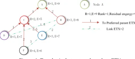
Energy assumption is the key issue of wireless sense network. Reference [6] focuses on minimizing the average energy consumption. The metric ETX is taken into account and energy-efficient routes are constructed based on the link reliability. A small number of nodes with a high ETX or close to the border routers may have to forward most of the traffic. As shown in Figure 1, a DAG is built on ETX. D can select C or B as the next hop. C should be preferred because it provides the lowest cumulative ETX to the sink. However, if all nodes produce the same amount of traffic, B should be the best choice to balance energy consumption. In [19] authors divide traffic into fixed rate and random rate, and transfers routing problem into linear planning problem in order to maximize network lifetime. It supposes that all nodes are fixed and the topology changes are slow. What’s more, it only presents a centralized algorithm and could not support distribution situations. Reference [20] divides energy sources into three kinds: mains-powered, primary batteries, energy scavengers, and presents calculation standard for every kind of power-supply way. By dynamically adjusting the transmission power of the sensor, the time insensitive packet is transmitted at a lower power to reduce the energy consumption, and real-time packets are transmitted at a high power. Although this solution is energy efficient for a single node, it does not give a global solution and does not maximize the network lifetime.

Figure 1. Topological structure based on ETX

proposed, namely, FLR (fast local repair), ELB (energy load balancing), and their combination FLR-ELB. Then authors apply them to IPv6 communication stack for Internet of Things. In [24], authors propose a neighbor node disjoint multipath (NDM) solution, which is proved more efficient when the intermediate node or link failures. In [30], authors propose Cooperative-RPL, which created different instances based on different sensing tasks. Nodes in different instances are responsible for forwarding different data. In this way, energy consumption is reduced compared to standard RPL.

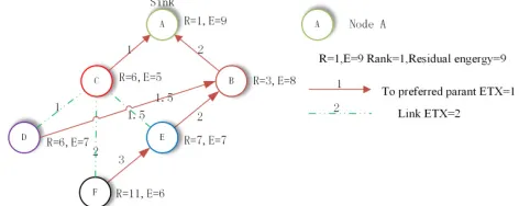
Figure 2. Network topology constructed according to the residual energy

Figure 2 constructs DAG based on the residual energy. F chooses E or C as a next hop. Even though the link quality of E is very low (ETX=3), it will be chosen as the parent owing to its residual energy is greater. This will increase the number of data package retransmission of F. According to the figure, C is a more appropriate choice.

2.4 End-to-End Delay

In many applications, energy effect and end-to-end delay are related. In order to increase the lifetime of battery-provided sensor, it had better close the wireless transceiver. Thus the data can’t arrive at the objective node in time, which can increase end-to-end time. To increase the network lifetime, we should use high-efficiency duty-cycled factor, which is bound to influence the system delay. High-efficiency means the increase of communication time. It will increase the single-hop delay. Under the circumstance of multi-hop, the end-to-end delay will be increased.

In [25] authors study the problem of network delay with low duty cycle and compare it with the RPL based on ETX. At the same time, it expands the duty cycle of ContikiMAC to support different sleep modes. However, it only uses simple delay metric but not considering the quality of the link and not building efficient energy metric mode. It fails to improve the other performances of the network and isn’t verified in a real environment. In [26] authors use the residual energy and transmission delay as the basis of the next hop choice. In some ways, it considers the network lifetime and end-to-end delay and optimizes the network by ant colony optimization. However, the author didn’t consider about the multipath support. Some nodes still may fail because of too much energy consumption. In [27] authors use fuzzy logic to design objective function and considers about node and link measurement, namely, end-to-end delay, hops, ETX and LQI. This algorithm support the quality of service in static and dynamic network environment, and improve the reliability and average delay of the network. The author ignores the node energy consumption, not considering the network lifetime. In [28], opportunistic routing is proposed, which may probably obtain better load balance. Data forward decision depends on the receiver rodes, rather than the sender nodes.

3. ADAPTIVE MULTIPATH TRAFFIC LOADING BASED ON RPL, AMTL-RPL

This section present an Adaptive Multipath Traffic Loading distribution method based on RPL. We realize the entire network’s energy balance and reduce the end-to-end delay by evaluating the energy consumption and cache utilization of bottleneck nodes in the network.

The first concern is the energy balance of the network. According to the idea of multipath transmission, in order to ensure the residual energy balance of the subsequent nodes, the sending node will transmit its data through multiple paths. This method will lead to multiple bottleneck nodes in the network, and makes it necessary to maintain the information of multiple bottleneck nodes. This section describes how to calculate the residual energy of the bottleneck node and how to allocate its transmission traffic. Specifically, we first analyze the basic energy consumption of the node, and then according to the Pareto evaluation model [29] to give the measurement of node’s energy distribution. Afterwards, we analyze the node’s energy consumption situation based on multipath distribution and finally propose the best plan for traffic distribution.

3.1.1. Node energy consumption model

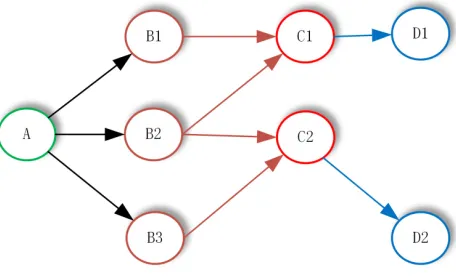
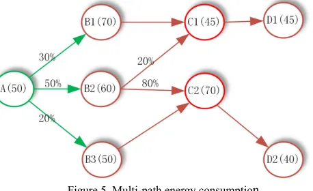
Let’s take the network topology of Figure 3 for example. Node A is the sending node, B1, B2 and B3 are its parent nodes; C1 and C2 are bottleneck nodes.

Figure 3. Node’s energy consumption

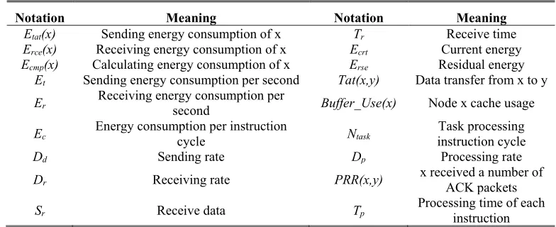
Node’s consumption can be classified as three parts, receiving consumption of new data, calculation consumption and sending consumption. We take node C1 as an example to calculate the three different kinds of energy consumption. The notations used in the article are shown in Table 1.

Step 1: node C1 receives the data which the descendant node sends; its energy consumption mainly comes from the consumption by receiving data:



= ×

= () 1

1 1 1

) , (

) , ( )

(

C b Parents

r r

D E c b PRR

c b Tat c

Erce (1)

Step 2: node C1 handles the cache queue; we can calculate its energy consumption by:

E_cmp( c ) =N₁ task(Buffer Use c_ ( ))₁ ×E_c (2)

Step 3: node C1 sends data to its descendant nodes after finish processing the cache queue which energy consumption is:

1 1

1

( , ) ( )

( , )

t tat

d E Tat c d

E c

PRR c d D

= × (3)

Thus, node C1’s residual energy is:

Here, _{( )} 1 c rse

E represents the residual energy after handling transmission task or the energy used to clear up the cache. This metric can affect the route choice of bottleneck nodes.

Table 1. Notation used in the article

Notation Meaning Notation Meaning

Etat(x) Sending energy consumption of x Tr Receive time

Erce(x) Receiving energy consumption of x Ecrt Current energy

Ecmp(x) Calculating energy consumption of x Erse Residual energy

Et Sending energy consumption per second Tat(x,y) Data transfer from x to y

Er Receiving energy consumption per _second Buffer_Use(x) Node x cache usage

Ec Energy consumption per instruction _cycle Ntask _{instruction cycle} Task processing

Dd Sending rate Dp Processing rate

Dr Receiving rate PRR(x,y) x received a number of _{ACK packets}

Sr Receive data Tp Processing time of each _instruction

3.1.2 The metric definition of energy balance

The amount of data transmission plays an important role for the whole network’s transmission rate. Even given global information, choosing an optimized energy balance algorithm is still a challenging. This paper takes multipath to balance the overload of network’s traffic.

According to RPL protocol, once DODAG has been constructed, all the traffic would transmit through one path until the network topology changed. To ensure maximum network lifetime, we need to improve DODAG which means making multi-path available. One node could distribute traffic to multiple parent nodes instead of the preferred one. This ensures that all of parents can be energy balance. We distribute data among different parent nodes to make sure the overload of the subsequent bottleneck nodes residual energy become balanced. In this paper, we consider the time of the first node to run out of energy as the whole network's lifetime.

In fact, bottleneck nodes will consume energy no matter we choose which node as the preferred parent. In order to ensure a more efficient evaluation of whether the bottleneck node is energy-balancing, it is necessary to evaluate the degree of dispersion of the remaining energy consumption of these nodes. Based on the relevant knowledge on math area, we use range, average deviation, standard deviation to assess data dispersion degree. Nevertheless, we found that these metrics couldn’t embody the distribution of bottleneck nodes’ remaining energy consumption through plenty of tests.

To estimate the distribution of bottleneck nodes’ energy consumption precisely, this paper gives the measurement of energy distribution equilibrium degree based on Pareto’s evaluation model [26].

The definition of energy of dispersion: Assume the rational number set represents sensor energy,

a

≥

0

n 2 1

= i i i

ED



Here,

) ( / 1

)) ( /(

1 2

A D

A E ai

i= −

ϖ

2

−

= , E(A)= A₁/n , _⋅x represents the

norm of x.

Table2. Comparison of several discrete degree metrics

Figure 4. Distribution of values

Firstly, we demonstrate numerical evaluations to compare their differences. 200 numbers from 1 to 100 are randomly selected, and calculated these measure values individually. The test goes 1000 times and records the maximum value, the minimum value and the average value. Here goes the result as Table 2 and Figure 4.

The above table shows the ED can express the data dispersion degree pretty well and reflect the fluctuation degree more clearly.

Furthermore, we compare these measurement standards based on RPL protocol. There are 100 nodes in the tests and each node has the same initial energy. We converted the energy into 100 units for simplification.

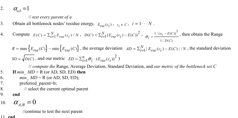
According to the RPL protocol, the preferred parent node needs to be selected firstly. For each possible parent node (that is, the Rank of the neighbor is smaller than that of itself), a node will take the following steps:

Step 1: Calculate bottleneck nodes’ measurement set (range-R、average deviation-AD、 standard deviation-SD and energy of dispersion-ED) through parent nodes broadcast. It will send all the traffic to that parent node and save the minimum value (Line 4);

Step 2: Calculate its own lifetime and make sure itself won’t become another new bottleneck node when choosing this father node (Line 5);

Step 3: Remove the traffic that arrive at that parent node and test other nodes. Make sure all the parent nodes have been tested before making the decision (Line 10);

Step 4: Select the preferred parent nodes. The node maximizes the lifetime of the bottleneck with the minimum lifetime (Line 6, 7, 8).

The main idea is listed in algorithm 1.

Algorithm 1 Evaluation different metrics based on RPL protocol

Input: the sender node a; the candidate parent set of a, parent(a); the bottleneck set, C; and its number N

Output: the preferred parent of a

Initializationmin_ MD =100000;

1. for

b parent a

∈

( )

measurement maximum minimum average

Range 98.6920 96.3815 97.5278

Average Deviation 40.4198 9.3249 26.5953

Standard Deviation 28.7187 9.3249 28.5178

2. , 1 a b α =

// test every parent of a

3. Obtain all bottleneck nodes’ residue energy, E_{rse i}( )c , c_i∈C, i= ⋅ ⋅ ⋅1 N.

4. Compute E C( )=_iN₌₁E_{rse i}( ) /c N, D C( )=_iN₌₁(E_{rse i}( )c −E C( ))2, 1 / ( ( ))2 1 / ( ) ϖi= ai−E C

D C

, then obtain the Range

{

}

{

}

max ( ) min ( )

= −

R E_rse C E_rse C , the average deviation AD=_iN₌₁|E_{rse i}( )c −E C( ) | /N, the standard deviation

( ) =

SD D C , and our metric ED=n_i=1ϖ_i⋅(E_{rse i}( ))c 2)

// compute the Range, Average Deviation, Standard Deviation, and our metric of the bottleneck set C

5. Ifmin_ MD > R (or AD, SD, ED) then

6. min_ MD =R (or AD, SD, ED); 7. preferred_parent=b;

8. // select the current optimal parent 9. end

10.

α

=

0

//continue to test the next parent 11.end

The above algorithm is used to choose preferred parent nodes based on single-path circumstances. We should give min_MD as large as possible to guarantee the value won’t smaller than the ED value under the real circumstances.

When the first node used up its energy, the experiment stops and records the bottleneck nodes’ energy. We achieve the average value through 1000 times and the results are as Table 3.

The evaluation verifies the ED can evaluate the imbalance degree of network nodes energy consumption well.

3.1.3 Multi-path energy consumption

If we use αx,y as the traffic ratio of node x send to its parent node y, then the bottleneck node’s

traffic is the traffic ratio that node a sends to three parent nodes individually multiplies the traffic ratio that they retransmit to bottleneck nodes , and then add them up. More generally, the expression should be:

, ( ) , ,

a c b Parents a a b b c

α =



(6)

Table 3. The compare results for several dispersion degrees

measurement maximum minimum average

Range 71.0600 69.9184 71.0588

Average 27.7367 6.1617 27.7151

Standard 28.8025 6.1617 28.8007

ED 1.0438e+05 574.5076 678.3107

We analyzed bottleneck nodes’ energy consumption based on multi-path distribution strategy in this section. As we know, nodes will send packets to several parent nodes through links with different quality, namely, nodes will transmit traffic through several paths, and hence, the energy that be consumed will depend traffic that sent to the each parent node. First, we elaborate how to calculate the bottleneck nodes’ remaining energy consumption under multi-path environment.

In Figure 5, node A is the sending node, its parent nodes are B1, B2 and B3, and bottleneck nodes are C1 and C2. For node C1, it receives 100% traffic of B1 and 20% of B2. The real traffic of C1 is:30%+50%×20%. Similarly, the real traffic of C2 is: 20%+50%×80%.

, ,

( )

( , ) ( , )

( , )

( , ) ( , )

a b b c

b Parents a

Tat a b Tat b c

Tat a c

PRR a b PRR b c

α α

∈

=



(7)

So, in terms of bottleneck node C1 equation (1) and (3) will turn to be:

1 1

( ) ( , ) r rce

r E

E c Tat a c

D

1 1

1

1 ( )

1 ( , ) ( )

( , )

c d t

tat d Parents c

d

Tat c d E

E c

PRR c d D

α ⋅

∈

×

=



In this case, the energy consumption of bottleneck node C1 is:

1 1

1 1 1 1 1

, 1

d (c )

1 ( ) ( ) ( ) ( , ) ( _ ( )) + ( , ) ( , ) r

rce cmp tat task c

r

c d t

Parents

d E

E c E c E c Tat a c N Buffer Use c E

D

Tat c d E

PRR c d D

α ∈ + + = × + × × ×



The parameter in the above equation can be obtained before transmission except for distribution traffic ratio, so node A can assess the impact of the survival time of the bottleneck node.

Figure 5.Multi-path energy consumption

Each node can calculate the transmission ratio of arriving at bottleneck nodes in recursion way. Thus the real traffic that the bottleneck nodes obtain is:

3.2 Multi-path traffic distributions

According to RPL, nodes will separate traffic on every path available to guarantee the lifetime of each bottleneck node is balanced. To maximize the network lifetime, we can consider using a plain linear program to assign weights to each parent node to obtain the optimal solution. However, it’s apparently not suitable for sensor nodes that are limited in both storage and calculation resource.

This paper proposes a quick algorithm based on the metric mentioned above. Firstly, we convert metric ED to objective function (ED=f(ax1,c1,ax2,c2,…)) about ax,c depend on correlative math

knowledge, where ci belong to bottleneck node set, and xi belong to descendants of ci. The function

is the two order continuous differentiable function, which can be solved by linear programming. Then, we combine Newton’s as well as steepest descent method to propose one modified algorithm. This method could find one of the best group’s weights to send traffic by iteration test. At the same time, it can realize convergence as soon as possible and has quite well stability and little calculation. Algorithm 2 gives its formal description: the nodes decide whether it gets proper answer (Line1), if not, it is judged whether or not an accurate search can be performed (Line 2). If it could, the

direction would be ( ) ) ( 2 k k x f x f ∇ ∇ −

(Line 3). If couldn’t, it use negative gradient search direction

) (xk f ∇

− _{(Line 5). Then, adjust the step length (Line 7), acting on iteration (Line 8), until we get the}

optimum solution.

Algorithm 2 Energy balance based on multi-path

Input: object function ( _, , _, , ) 1 2 α α ⋅ ⋅ ⋅ f _{a b b c}

Output: _{, ,} ,₁ ,₂

αb c αb c ⋅ ⋅ ⋅ for energy balance

Initialization δ>0, α_{b c,} =random[0, 1] and _{( ) 1} , α

c bnk b∈ _{b c} = ,x0=αb c,₁,αb c,₂,⋅ ⋅ ⋅ , k=0

2. if ( ) ( ) ₀ 2 ( ) ∇ ⋅ ∇ > ∇ T f x_k f x_k

f xk

then

3. ( )

2 _{( )} ∇ = −

∇ f x k d k

f x k

4. else

5. d_k = −∇f x( _k)

6. end

7. ( )

2 ( )

λ = − −∇ ⋅

⋅ ∇ ⋅

T f x_k d_k

k T T

d_k f x_k d_k

;

8. x_k+1= x_k +λ_k ⋅d_k

9. k = k+1;

10. end

11. Return _xk

The advantage of the algorithm is that the iterative step size adjustment uses the method of precision searching for minimizing the quadratic function. The convergence rate is linear and can be guaranteed every time. When the maximum eigenvalue and the minimum eigenvalue of the Hessian matrix are close to each other, the descending velocity is the fastest. Particularly, when they are equal to each other, we can obtain the optimum solution just through only one iteration. Furthermore, the number of bottleneck nodes would change with the network. When the number of bottleneck increases, the energy consumption of x increases. At this time, we can use Quasi-Newton’s method to reduce the amount of calculation about Hessian matrix, namely,

2

2 2 2

1

( ) ( ) ( ) 1

( ) ( ) 1+ ( ) ( ) ( )

( ) ( ) ( )

T T

T T

k k k k k

k k T T T k k k k k

k k k k k k

s s y f x y

f x f x s y s y f x

s y s y s y

+

 ⋅ ∇ ⋅  _{ }

∇ = ∇ + _ _−  + ⋅∇

(11)

where

3.3 End-to-end delay optimization

This section studies how node’s cache impacts on end-to-end delay. We abstract the transmission procedure as Markov procedure and analyze the packet loss depend on bottleneck nodes’ remaining cache. Subsequently, we calculate the dispersion degree of the remaining cache size of the bottleneck nodes. Finally, we give the multi-path data distribution algorithm depends on the remaining cache size of the bottleneck nodes.

3.3.1 Data forwarding model and node transfer latency

The limited capacity of cache is a vital factor that influences the network performance. The efficiency of the cache directly affects the reliability and stability of the entire network, and also indirectly affects its survival time. The unreasonable routing protocol always leads to data gathering together at some nodes, which makes their cache overflow. More seriously, they can only receive data from descendant nodes, and can not be forwarded further. This "invalid operation" node greatly increases the end-to-end transmission time. On the other hand, if some node’s cache utilization rate is too high, that is, too many data frames in the node, and then its CPU will spend too much energy on receiving, handling and sending data. If these conditions continue, there will be a certain number of nodes will soon fail, resulting in network vacancies, which seriously undermine the network connectivity, extending the end-to-end delay.

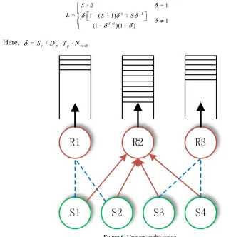
In Figure 6, S1 to S4 represent data sources, R1 to R3 represent relay nodes. If all the data sources select R2 to do data transmission, and that node will gradually become bottleneck nodes. Because of the restriction of cache, it must loss some data if the cache utilization rate achieves some level.

data packet arrives at nodes couldn’t be placed into cache pool, these packets will be lost. According to the queuing theory, nodes’ cache can have the desired value like:

1 1

/ 2 1

1 ( 1)

1

(1 )(1 )

S

S S

L S S

δ

δ δ δ

δ

δ δ

+ +

=

 

=_{ } − + + _

≠

 _{− −}



(12)

Here

,

Figure 6. Uneven cache usage

The remaining cache R: R=S-L. The remaining cache has a significant impact on the loss of packets. Nodes’ packet loss ratio is:

1 1/ ( 1) 1

(1 ) 1 1

R

R R p

δ

δ δ _δ

δ +

+ =

 

= − _≠

 ₋ 

(13)

Combine L with P, the resulting data packet’s average waiting time is:

1

(1 )

r p p task

L T

S p D T N

= −

− ⋅ ⋅

(14)

The waiting time of data packet is determined by L, P, Sr, Dp, Tp, Ntask. L and P can be solved by

the last four parameters. The last three parameters are determined by sensors. That is, they are constants. The average waiting time is mainly caused by the amount of receiving data. This means that a reasonable allocation of traffic can reduce end-to-end transmission time.

3.3.2 Waiting time for multi-path transmission nodes

The delay of end-to-end transmission is mainly based on the waiting time that data packet in the bottleneck nodes. As Figure 3, the bottleneck nodes’ traffic is ratio of traffic that node A sent to its three parent nodes individually multiples ratio of traffic that transmits to their bottleneck and add them up. Hence, the number of data received by the bottleneck node in the multi-path case is:

,

( , ) ( , )

r a c

S a c _{=α ⋅}Tat a c

(15)

,

1 ( , )(1 )

a c

r p p task

L D T

S a c p D T N

= = −

−

(16)

3.3.3 Multi-path traffic distribution

According to the above model, we propose a multi-path traffic distribution algorithm based on RPL to reduce the waiting time. This algorithm takes the use of greedy thoughts. A heuristic scheme is used to determine the weight of each associated parent node. Specifically, nodes divided distribute the traffic into N parts. Each part assigns to its parent node which can minimize the maximum delay among all of the bottleneck nodes.

Algorithm 3 gives the formal description, the main idea is to test all the parent nodes by greedy iteration, and find out the approximate optimal flow distribution scheme. Take Figure 3 as an example, Node A first allocates traffic evenly for each parent node, and then tests the smallest of the maximum waiting times in the bottleneck node by gradually adjusting the weight of the parent node. If the maximum waiting time can be reduced, it saves the current node and reinitializes traffic distribution so that other parent node can be tested. Finally, it assigns step length to the most appropriate parent node and restart to iteration, and find a reasonable flow distribution.

The selection of step size determines the optimal result of flow distribution and the energy consumption of the node. Using small step length can be able to obtain less waiting time of bottleneck nodes, while it strengthens the complexity of calculation. Conversely, the traffic distribution scheme is not reasonable enough. That is, we should set proper step length with regard to the real situation and request.

Algorithm 3 End-to-end delay based on multi-path

Input: the sender node A and its transmission quantity; the candidate parent set of A, parent(A) and its number ; the bottleneck set, C, and its number N; Δα

Output: all , a b α

1. fori=1 to 1 /Δα 2. min_time=10000;

3. All α_{a b,} =Tat a( ) /Num parent a( ( ));;

4. for b∈parent a( ) 5. _{αa b, =αa b, − Δα}

// test every step

6. obtain all bottleneck nodes’ waiting time _{T ci}( ), c_i∈C,i=1N, then

max_time=max{ ( )}_{T ci} 7. if max_time < min_time then

8. max_time=min_time;

9. min=b;

10. end

11. _{αa b,} =_{αa b,} + Δ_α

12. end

13. α_min=α_min− Δα

14. End

3.3.4 Adaptive traffic assignment algorithm

nodes’ waiting time to shorten the end-to-end delay (Line 4); if we consider the end-to-end delay first, call algorithm 3 (Line 6), when the delay smaller than the determined threshold, than change to algorithm 2.

Algorithm 4 Adaptive Multipath Traffic Loading

Input: Γ_edand Γ_de // Γ_ed is the threshold for energy dispersion of the network, Γ_de is the threshold utilization rate for delay of

bottleneck.

Output: _, , _, , 1 2 a_{b c} a_{b c} 

1. Case energy-first: 2. Call Algorithm 2 3. If ED<

ed Γ then 4. Call Algorithm 3 5. Case delay-first: 6. Call Algorithm 3 7. If D<Γ_de then

8. Call Algorithm 2 9. end

4. ANALYSIS OF THE PERFORMANCE

This section evaluates the performance of our algorithm. It mainly proves the network performance (load distribution, network lifetime, energy consumption, end-to-end delay, the stability of the route) using the former algorithm under different network sizes or with different cache in nodes.

4.1 Evaluation Environment

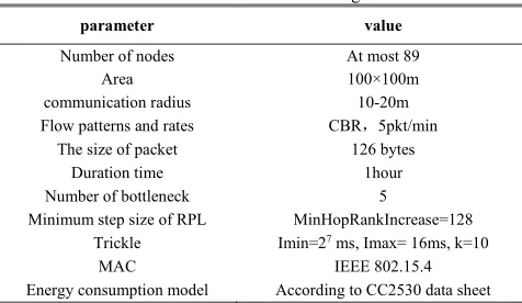
The experimental parameters are set as shown in Table 4.

Table 4. Parameter setting

parameter value

Number of nodes At most 89

Area 100×100m

communication radius 10-20m

Flow patterns and rates CBR，5pkt/min

The size of packet 126 bytes

Duration time 1hour

Number of bottleneck 5

Minimum step size of RPL MinHopRankIncrease=128 Trickle Imin=27 _{ms, Imax= 16ms, k=10}

MAC IEEE 802.15.4

Energy consumption model According to CC2530 data sheet

4.2 Analysis of the network performance

4.2.1 Network load distribution with different buffer size

retransmission will rise due to the loss of data. The smaller the cache is, the easier it will be full for the nodes closed to the center, which causes the loss of data. Figure 8a, 8c and 7a, 7c compared the energy consumption between algorithm 2 and algorithm 4. From the figures we can see that the network lifetime will be longer if we use energy balance to make the distribution of the energy more uniform. There’s no need to consider about the energy consumption of the sink node, since the sink node usually uses the mains-powered system instead of the battery-powered. We can also find from the figures that algorithm 2 has the best result. That is because it first considered the energy balance without end-to-end delay as the main factor. At the same time, the curve of this test is smooth. It shows that the load of nodes is almost the same if they are

Figure 7. Residual energy distribution (cache size 30). (a) for original RPL; (b) for algorithm 2; (c) for algorithm 4 of the same distance to the sink node. However, RPL cannot ensure this. As a result, our algorithm can efficiently balance the load of the packets which are sent by the network. It can better ensure the load balance if there are less nodes. In the actual situation, as time goes, there will be some bottleneck. Their processing speed will be slowing down obviously, resulting in the cache of its surrounding nodes to drop. If you use the algorithm we talked about in this essay, you’ll effectively remit the tension level of bottleneck nodes and the surrounding nodes.

Figure 8. Residual energy distribution (cache size 50). (a) for original RPL; (b) for algorithm 2; (c) for algorithm 4

4.2.2 Network-lifetime

Figure 9. Network lifetime in different size

4.2.3 Analysis of the end-to-end delay

Subsequently, we compare the delay between nodes based on algorithm 3, algorithm 4 and original RPL in Figure 10. According to the results, algorithm 3 needs the least time because it only focuses the transmission time between nodes and use the best route to do the timely data forwarding. It also extremely reduces the possibility of the loss of data and the low probability of data retransmission. Although algorithm 4 is not as effective as algorithm 3, its delay is still smaller than original RPL. It firstly considers the energy balance and ensures the network lifetime as long as possible. On the basis of this, it considers the cache utilization. However, the original RPL always do the packets forwarding by choosing preferred parent node. The choice of the parent node is determined by the OF function, which is determined by some metrics. As long as the topology does not change, the preferred parent node will not change. There is no guarantee of end-to-end delay.

From the figure we can see that there is irregular fluctuation of delay under different network sizes. It is respond to the position of nodes.

Figure 10. Network end-to-end delay in different size

4.2.4 The stability of the route

the control messages, the more energy it will consume. Moreover, the frequent changes will make the network unstable and will make the network topology worse. Above algorithm except original RPL make all parent nodes participate traffic forwarding without changing the preferred parent node. The preferred parent node will only change if it fails, and then the trigger timer will be reset. This will ensure network stability.

Figure 11. PDR in different network size

5. CONCLUSIONS

In this paper, we propose an Adaptive Multipath Traffic Loading based on RPL to meet the needs of energy consumption and end to end delay. First, we design an energy-balanced routing algorithm to improve the network lifetime. By establishing a practical model and proposing a standard of energy dispersion degree measurement, it can effectively determine the degree of energy balance of nodes. Based on this metric, we present a fast algorithm to obtain the optimal distribution of the data. The algorithm maintains the stability of parent set, so it improves the stability of the network.

Furthermore, in order to decrease end-to-end delay, we convert the data transmission model to M/M/1/S/FCFS model based on cache utilization, calculate the average waiting time of data, and then get the waiting time of the bottleneck node in the multi-path. Using the calculated time value, we propose a traffic allocation algorithm based on greedy thought, which can optimize the end-to-end delay.

Finally, taking into account the application needs of different scenarios, we integrate the two algorithms above. If the network prioritizes the survival time, priority is given to the energy balance, and then the end-to-end delay. If end-to-end delay is the mainly factor of the network, we consider about the cache utilization to decrease the loss of packets. The results indicate that three schemes all improve the reliability of routing, increase the network lifetime, decrease the end-to-end delay and decrease the times of DAG resetting.

It can be seen from the experiment; the nodes around the sink still consume more energy due to bear more traffic. They are still the bottlenecks of the entire network. In future work, the nodes around the sink will be optimized to maximize their survival time. Such measures include deploying more nodes around the sink, increasing their lifetime by turning off the Radio, increasing the transmission distance of a single hop, and even using mobile sink nodes to make the energy consumption of the entire network balance, extend the survival time of the network.

ACKNOWLEDGEMENTS

REFERENCES

[1] K. F. Li, "Smart home technology for telemedicine and emergency management," Springer. Journal of Ambient Intelligence & Humanized Computing, vol.4, no.5, pp.535-546, May.2012.

[2] T. Sanislav, G. Mois, S. Folea, L. Miclea, "A cloud-based Cyber-Physical System for environmental monitoring," In proc. MECO, Budva, Montenegro, 2014, pp.6-9.

[3] S. Wang, J. Xing, J. Li, Q. Yang, "A decentralized flat control system for intelligent building," in proc. CCDC, Qingdao, China,2015, pp.2622 - 2627.

[4] P. Thubert, T. Winter, A. Brandt, J. Hui, R. Kelsey, P. Levis. (2012, March). RPL: IPv6 Routing Protocol for Low-Power and Lossy Networks. [Online]. Available: https://www.rfc-editor.org/info/rfc6550.

[5] K. Andrea, R. Simon, "Design and Evaluation of an RPL-based Multi-Sink Routing Protocol for Low-Power and Lossy Networks," in

proc. MSWiM'15, Cancun, Mexico, 2015, pp.141-150.

[6] D.S.J.De Couto, D. Aguayo, J. Bicket, R. Morris, "a high-throughput path metric for multi-hop wireless routing," Springer. Wireless Networks, vol.11, no.4, pp.419-434, Jul. 2005.

[7] M. Conti, E. Gregori, G. Maselli, "Reliable and efficient forwarding in ad hoc networks," Elsevier. Ad Hoc Networks, vol.4, no.3, pp.398-415, May. 2006.

[8] M. Radi, B. Dezfouli, K.A. Bakar, M. Lee, "Multipath Routing in Wireless Sensor Networks: Survey and Research Challenges," MPDI. Sensors, vol.12, no.1, pp.650-685, Dec. 2012.

[9] K.S. Hong, L. Choi, "DAG-based multipath routing for mobile sensor networks," in proc. ICT, Seoul, South Korea, 2011, pp.261-266. [10] J. Nurmio, E. Nigussie, C. Poellabauer, "Equalizing energy distribution in sensor nodes through optimization of RPL," in proc.

CIT/IUCC/DASC/PICOM, Liverpool, UK, 2015, pp. 83-91.

[11] Y. Chen, N. Nasser, "Energy-balancing multipath routing protocol for wireless sensor networks," in proc. Quality of Service in Heterogeneous Wired/wireless Networks, Waterloo, Ontario, 2006, pp.21-24.

[12] B. Yahya, J. Ben-Othman, "REER: Robust and Energy Efficient Multipath Routing Protocol for Wireless Sensor Networks", in proc. GLOBECOM, Honolulu, HI, 2009, pp.1-7.

[13] X. Liu, J. Guo, G. Bhatti, P. Orlik, "Load balanced routing for low power and lossy networks," in proc. WCNC, Shanghai, China, 2013, pp.2238-2243.

[14] M. N. Moghadam, H. Taheri, "High throughput load balanced multipath routing in homogeneous wireless sensor networks," in proc. ICEE, Tehran, Iran, 2014, pp. 1516-1521.

[15] B. Pavković, F. Theoleyre, A. Duda, "Multipath opportunistic RPL routing over IEEE 802.15.4," in Proc. MSWIM2011, Miami, Florida, 2011, pp.179-186.

[16] T. Grubman, Y.A. Şekercioğlu, N. Moore, "Opportunistic Routing in Low Duty-Cycle Wireless Sensor Networks," Acm Trans. Sensor Networks, vol.10, no.4, pp.1-39, Jun. 2014.

[17] R. Kacimi, R. Dhaou, A. L. Beylot, "Load balancing techniques for lifetime maximizing in wireless sensor networks," Elsevier. Ad Hoc Networks, vol.11, no.8, pp.2172-2186, Nov. 2013.

[18] O. Iova, F. Theoleyre, T. Noel, "Using multiparent routing in RPL to increase the stability and the lifetime of the network," Elsevier. Ad Hoc Networks, vol.29, pp.45-62, Jun. 2015.

[19] J. H. Chang, L. Tassiulas, "Maximum lifetime routing in wireless sensor networks," IEEE/ACM. Trans.Networking, vol.12, no.4, pp.609-619, Sep. 2004.

[20] C. Systems, M. Kim, K. Pister, N. Dejean, D. Barthel. (2012, March). Routing Metrics Used for Path Calculation in Low-Power and Lossy Networks. [Online]. Available. https://www.rfc-editor.org/info/rfc6551.

[21] H. Liu, Z.L. Zhang, J. Srivastava, V. Firoiu, "PWave: A Multi-source Multi-sink Anycast Routing Framework for Wireless Sensor Networks," in proc. IFIP-TC6, Atlanta, GA, 2007, pp.179-190.

[22] L. H. Chang, T. H. Lee, S. J. Chen, C. Y. Liao, "Energy-Efficient Oriented Routing Algorithm in Wireless Sensor Networks," in proc. SMC, Manchester, UK, 2013, pp.3813-3818.

[23] Q. Le, T. Ngo-Quynh, T. Magedanz, "RPL-based multipath routing protocols for Internet of Things on wireless sensor networks," in proc. ATC, Hanoi, Vietnam, 2014, pp. 424-429.

[24] A. K. M. Hossain, C. J. Sreenan, R. D. P. Alberola, "Neighbour-disjoint multipath for low-power and lossy networks," ACM Trans. Sensor Networks , vol.12, no. 3, pp.23, Aug. 2016.

[25] P. Gonizzi, R. Monica, G. Ferrari, "Design and evaluation of a delay-efficient RPL routing metric," in proc. IWCMC, Sardinia, Italy, 2013, pp.1573-1577.

[26] B. Mohamed, F. Mohamed, "QoS Routing RPL for Low Power and Lossy Networks," Sage. International Journal of Distributed Sensor Networks, vol.11, vol.11, pp.1-10, Nov. 2015.

[28] M. Michel, S. Duquennoy, B. Quoitin, "Load-Balanced Data Collection through Opportunistic Routing," in proc. DCOSS, Fortaleza, Brazil, 2015, pp. 62-70.

[29] X. C. Hao, M. Q. Wang, S. Hou, Q. Q. Gong, B. Liu, "Distributed Topology Control and Channel Allocation Algorithm for Energy Efficiency in Wireless Sensor Network: From a Game Perspective," EBSCO. Wireless Personal Communications, vol.80, no.4, pp.1557-1577, Feb. 2015.