Modeling Quantum Behavior in the Framework of Permutation
Groups
VladimirKornyak1,
1Laboratory of Information Technologies, Joint Institute for Nuclear Research, 141980 Dubna, Moscow Region, Russia
Abstract.Quantum-mechanical concepts can be formulated in constructive finite terms without loss of their empirical content if we replace a general unitary group by a unitary representation of a finite group. Any linear representation of a finite group can be realized as a subrepresentation of a permutation representation. Thus, quantum-mechanical prob-lems can be expressed in terms of permutation groups. This approach allows us to clarify the meaning of a number of physical concepts. Combining methods of computational group theory with Monte Carlo simulation we study a model based on representations of permutation groups.
1 Introduction
Since the time of Newton, differential calculus demonstrates high efficiency in describing physical
phenomena. However, the infinitesimal analysis introduces infinities in the physical theories. This is often considered as a serious conceptual flaw: recall, for example, Dirac’s frequently quoted claim that the most important challenge in physics is “to get rid of infinity”. Moreover, differential calculus,
being, in fact, a kind of approximation, may lead to descriptive losses in some problems – an illus-trative example is given below in Sec. 3.1. In the paper, we describe a constructive version of the quantum formalism that does not involve any concepts associated with actual infinities.
The main part of the paper starts with Sec. 2, which contains a summary of the basic concepts of the standard quantum mechanics with emphasis on the aspects important for our purposes.
Sec. 3 describes a constructive modification of the quantum formalism. We start with replacing a continuous group of symmetries of quantum states by a finite group. The natural consequence of this replacement is unitarity, since any linear representation of a finite group is unitary. Further, any finite group is naturally associated with some cyclotomic field. Generally, a cyclotomic field is a dense subfield of the field of complex numbers. This can be regarded as an explanation of the presence of complex numbers in the quantum formalism. Any linear representation of a finite group over the associated cyclotomic field can be obtained from a permutation action of the group on vectors with natural components by projecting into a suitable invariant subspace. All this allows us to reproduce all the elements of the quantum formalism in invariant subspaces of the permutation representations.
In Sec. 4 we consider a model of quantum evolution inspired by the quantum Zeno effect – the
most convincing manifestation of the role of observation in the dynamics of quantum systems. The model represents the quantum evolution as a sequence of observations with unitary transitions between them. The standard quantum mechanics assumes a single deterministic unitary transition between observations. In our model we generalize this assumption. We treat a unitary transition as a kind
of gauge connection – a way of identifying indistinguishable entities at different times. A priori,
any unitary transformation can be used as a data identification rule. So, we assume that all unitary transformations participate in transitions between observations with appropriate weights. We call a unitary evolutiondominant if it provides the maximum transition probability.1 The Monte Carlo simulation shows a sharp dominance of such evolutions over other evolutions. To compare with a continuous description, we present also the Lagrangian of the continuum approximation of the model.
2 Formalism of quantum mechanics
Here is a brief outline of the basic concepts of the quantum mechanics. We divide these concepts into three categories:states,observations and measurements, andtime evolution.
2.1 States
Apure quantum stateis a ray in a Hilbert spaceHover the complex fieldC, i.e., anequivalence classof vectors |ψ ∈ Hwith respect to theequivalence relation |ψ ∼a|ψ, wherea∈C,a0. We can reduce the equivalence classes bynormalization: |ψ ∼ eiα|ψ,ψ=1, α∈R. Finally, we can eliminate the phase “degree of freedom”αby transition to the rank oneprojectorΠψ=|ψψ|, which is a special case of adensity matrix.
Amixed quantum stateis described by ageneral density matrixρcharacterized by three prop-erties: (a)ρ = ρ†, (b) ψ|ρ|ψ ≥ 0 for any |ψ ∈ H, (c) trρ = 1. In fact, any mixed state is a
weighted mixture of pure states, i.e., its density matrix can be represented as a weighted sum of rank one projectors. We will denote the set of all density matrices byD(H).
The Hilbert space of acomposite system,XY =X×Y, is the tensor product of the Hilbert spaces
for its constituents: HXY =HXHY. Thestates of a composite system,D(HXY), are classified into two types: separableandentangled states. The set of separablestates, DS(HXY), consists of the statesρXY ∈ D(HXY) that can be represented as weighted sums of the tensor products of states of the constituents:ρXY=kwkρkX
ρkY, wk≥0, kwk=1. The set ofentangledstates,DE(HXY), is by definition the complement ofDS(HXY) in the set of all states:DE(HXY)=D(HXY)\ DS(HXY).
2.2 Observations and measurements
The terms ‘observation’ and ‘measurement’ are often used as synonyms. However, it makes sense to separate these concepts: we treat observation as a more general concept which does not imply, in contrast to measurement, obtaining numerical information.
Anobservationis the detection (“click of detector”) of a system found in the stateρin the subspace S ≤ H. The mathematical abstraction of the “detector in the subspace”Sof a Hilbert space is the operator of projection,ΠS, into this subspace. The result of quantum observation is random and its
statistics is described by a probability measure defined on subspaces of the Hilbert space. Any such measureµ(·) must be additive on any set of mutually orthogonal subspaces of a Hilbert space: if, e.g., AandBare mutually orthogonal subspaces, then µspan (A,B) = µ(A)+µ(B). Gleason proved [1] that, except the case dimH =2, the only such measures have the formµρ(S)=tr (ρΠS), whereρis an arbitrary density matrix. If, in particular,ρdescribes a pure state,ρ=|ψψ|, andSis one-dimensional,S=span (|ϕ), we come to the familiar Born rule: tr (ρΠS)=PBorn=|ϕ|ψ|2.
Ameasurementis a special case of observation, when the partition of a Hilbert space into mutually orthogonal subspaces is provided by a Hermitian operatorA. Any such operator can be written as
A =kakΠek, wherea1,a2, . . . ∈ Ris thespectrumof A, ande1,e2, . . .is an orthonormal basis of eigenvectorsofA. “Click of the detector”Πek is interpreted as that theeigenvalue akis the result of the measurement. The mean for multiple measurements tends to theexpectation valueof Ain the stateρ: Aρ=tr (ρA).
1In fact, the principle of least action in physical theories implies the selection of dominant evolutions among all possible
of gauge connection – a way of identifying indistinguishable entities at different times. A priori,
any unitary transformation can be used as a data identification rule. So, we assume that all unitary transformations participate in transitions between observations with appropriate weights. We call a unitary evolutiondominant if it provides the maximum transition probability.1 The Monte Carlo simulation shows a sharp dominance of such evolutions over other evolutions. To compare with a continuous description, we present also the Lagrangian of the continuum approximation of the model.
2 Formalism of quantum mechanics
Here is a brief outline of the basic concepts of the quantum mechanics. We divide these concepts into three categories:states,observations and measurements, andtime evolution.
2.1 States
Apure quantum stateis a ray in a Hilbert spaceHover the complex fieldC, i.e., anequivalence classof vectors|ψ ∈ Hwith respect to theequivalence relation |ψ ∼a|ψ, wherea∈C,a0. We can reduce the equivalence classes bynormalization: |ψ ∼ eiα|ψ,ψ=1, α∈R. Finally, we can eliminate the phase “degree of freedom”αby transition to the rank oneprojectorΠψ=|ψψ|, which is a special case of adensity matrix.
Amixed quantum stateis described by ageneral density matrixρcharacterized by three prop-erties: (a)ρ = ρ†, (b) ψ|ρ|ψ ≥ 0 for any |ψ ∈ H, (c) trρ = 1. In fact, any mixed state is a
weighted mixture of pure states, i.e., its density matrix can be represented as a weighted sum of rank one projectors. We will denote the set of all density matrices byD(H).
The Hilbert space of acomposite system,XY=X×Y, is the tensor product of the Hilbert spaces
for its constituents: HXY =HXHY. Thestates of a composite system,D(HXY), are classified into two types: separableandentangled states. The set of separablestates, DS(HXY), consists of the statesρXY ∈ D(HXY) that can be represented as weighted sums of the tensor products of states of the constituents:ρXY=kwkρkX
ρkY, wk≥0, kwk=1. The set ofentangledstates,DE(HXY), is by definition the complement ofDS(HXY) in the set of all states:DE(HXY)=D(HXY)\ DS(HXY).
2.2 Observations and measurements
The terms ‘observation’ and ‘measurement’ are often used as synonyms. However, it makes sense to separate these concepts: we treat observation as a more general concept which does not imply, in contrast to measurement, obtaining numerical information.
Anobservationis the detection (“click of detector”) of a system found in the stateρin the subspace S ≤ H. The mathematical abstraction of the “detector in the subspace”Sof a Hilbert space is the operator of projection,ΠS, into this subspace. The result of quantum observation is random and its
statistics is described by a probability measure defined on subspaces of the Hilbert space. Any such measureµ(·) must be additive on any set of mutually orthogonal subspaces of a Hilbert space: if, e.g., A andBare mutually orthogonal subspaces, then µspan (A,B) = µ(A)+µ(B). Gleason proved [1] that, except the case dimH=2, the only such measures have the formµρ(S)=tr (ρΠS), whereρis an arbitrary density matrix. If, in particular,ρdescribes a pure state,ρ=|ψψ|, andSis one-dimensional,S=span (|ϕ), we come to the familiar Born rule: tr (ρΠS)=PBorn=|ϕ|ψ|2.
Ameasurementis a special case of observation, when the partition of a Hilbert space into mutually orthogonal subspaces is provided by a Hermitian operatorA. Any such operator can be written as
A = kakΠek, wherea1,a2, . . . ∈ Ris thespectrumof A, and e1,e2, . . .is an orthonormal basis of eigenvectorsofA. “Click of the detector”Πek is interpreted as that theeigenvalue akis the result of the measurement. The mean for multiple measurements tends to theexpectation valueof Ain the stateρ: Aρ=tr (ρA).
1In fact, the principle of least action in physical theories implies the selection of dominant evolutions among all possible
(“virtual”) evolutions. The apparent determinism of these evolutions can be explained by the sharpness of their dominance.
2.3 Time evolution
Thetime evolutionof a quantum system is a unitary transformation of data between observations. For a density matrix, the unitary evolution takes the form
ρ
t =Uttρ
tU†tt, (1)whereρt is the state after observation at the timet, ρt is the statebeforeobservation at the time
t, andU
ttis the unitary transition between the observation timestandt. In the standard quantum
formalism, the time is considered as a continuous parameter, and the relation (1) becomes thevon Neumann equationin the infinitesimal limit. The evolution of a pure state can be written as |ψt =
Utt|ψt, and the corresponding infinitesimal limit is theSchrödinger equation. To emphasize the role
of the observation in the quantum physics, we note that the unitary evolution is simply a change of coordinates in the Hilbert space and it is not sufficient to describe observable physical phenomena.
2.4 Emergence of geometry within large Hilbert space via entanglement
The quantum-mechanical theory does not need the geometric space as a fundamental concept – every-thing can be formulated using only the Hilbert space formalism. In this view, the observed geometry must emerge as an approximation. The currently popular idea [2–4] of the emergence of geometry within a Hilbert space is based on the notion of entanglement. Briefly, the scheme of extracting ge-ometric manifold from the entanglement structure of a quantum stateρin a Hilbert space H is as follows:
• The Hilbert space decomposes into a large number of tensor factors: H = xHx, x ∈ X. Each factor is treated as a point (or bulk) of geometric space to be built. A graph G– calledtensor network– with verticesx∈Xand edges {x, y} ∈X×Xis introduced.
• The edges ofGare assignedweightsbased on ameasure of entanglement, a function that vanishes on separable states and is positive on entangled states. A typical such measure is themutual infor-mation: Iρxy
= S(ρx)+Sρy
−Sρxy
, whereρx denotes the result of taking traces ofρover all tensor factors except for the x-th (and similarly forρy, ρxy); S(a) = −traloga is thevon Neumann entropy. The graphGis supplied with a metric derived from the weights of the edges. • Finally, the graphGis approximately isometrically embedded in a smooth metric manifold of an as
small as possible dimension using algorithms like themultidimensional scaling(MDS).
3 Constructive modification of the quantum formalism
David Hilbert, a prominent advocate of the free use of the concept of infinity in mathematics, wrote the following about the relation of the infinite to the reality: “Our principal result is that the infinite is nowhere to be found in reality. It neither exists in nature nor provides a legitimate basis for rational thought – a remarkable harmony between being and thought.” Adopting this view, we reformulate the quantum formalism in constructive finite terms without distorting its empirical content [5–7].
3.1 Losses due to continuum and differential calculus
Differential calculus (including differential equations, differential geometry, etc.) forms the basis
of the mathematical methods in physics. The applicability of the differential calculus is based on
the assumption that any relevant function can be approximated by linear relations at small scales. This assumption simplifies many problems in physics and mathematics, but at the cost of loss of completeness.
invertibility for each element. There are two most common additional assumptions that make the notion of a group more meaningful: (a)the group is a differentiable manifold – such a group is calledLie group; (b)the group is finite. The empirical physics is insensitive to the assumption (b) – ultimately, any empirical description is reduced to a finite set of data. On the contrary, the assumption (a) implies severe constraints on the possible physical models.
The problem of the classification of the simple groups2 under the assumption (a) turned out to be rather easy and was solved by two people (Killing and Cartan) in a few years. The result is four infinite series:An,Bn,Cn,Dn; and five exceptional groups:E6,E7,E8,F4,G2.
The solution of the classification problem under the assumption (b) required the efforts of about a
hundred people for over a hundred years [8]. But the result –“the enormous theorem”– turned out to be much richer. The list of finite simple groups contains 16+1+1 infinite series:
• groups of Lie type:
An(q),Bn(q),Cn(q),Dn(q),E6(q),E7(q),E8(q),F4(q),G2(q),
2Anq2,2Bn22n+1,2Dnq2,3D4q3,2E6q2,2F422n+1,2G232n+1;
• cyclic groups of prime order, Zp; • alternating groups, An, n≥5;
and 26sporadic groups:M11,M12,M22,M23,M24,J1,J2,J3,J4,Co1,Co2,Co3,
Fi22,Fi23,Fi24,HS,McL,He,Ru,S uz,ON,HN,Ly,Th,B,M.
Note that finite groups have an advantage over the Lie groups in the sense that in the empirical appli-cations any Lie group can be modeled by some finite group, but not vice versa.
3.2 Replacing a unitary group by a finite group
The main non-constructive element of the standard quantum formalism is the unitary groupU(n), a set of cardinality of the continuum.
Formally, the groupU(n) can be replaced by some finite group which is empirically equivalent to U(n) as follows. From the theory of quantum computing it is known thatU(n) contains a dense finitely generated – and, hence, countable – matrix subgroupU∗(n). The groupU∗(n) isresidually finite, i.e., it has a reach set of non-trivial homomorphisms to finite groups.
In essence, it is more natural to assume that, at the fundamental level, there are finite symmetry groups and that theU(n)’s are just continuum approximations of their unitary representations.
The following properties of the finite groups are important for our purposes: • any finite group is a subgroup of asymmetric group,
• any linear representation of a finite group isunitary,
• any linear representation is a subrepresentation of somepermutation representation.
3.3 “Physical” numbers
The basic number system in quantum formalism is the complex fieldC. This non-constructive field can be obtained as a metric completion of many algebraic extensions of the rational numbers. We consider here constructive numbers that are closely related to the finite groups and are based on two primitives with clear intuitive meanings:
1. natural numbers(“counters”):N={0,1, . . .};
2. kthroots of unity3(“algebraic form of the idea ofk-periodicity”):r
k|rkk=1.
These basic concepts are sufficient to represent all physically meaningful numbers.
2The simple groups, i.e., groups that do not contain nontrivialnormal subgroups, are “building blocks” for all other groups. 3There arekdifferentkth roots of unity. Akth root of unity is calledprimitiveifrm
invertibility for each element. There are two most common additional assumptions that make the notion of a group more meaningful: (a) the group is a differentiable manifold – such a group is calledLie group; (b)the group is finite. The empirical physics is insensitive to the assumption (b) – ultimately, any empirical description is reduced to a finite set of data. On the contrary, the assumption (a) implies severe constraints on the possible physical models.
The problem of the classification of the simple groups2 under the assumption (a) turned out to be rather easy and was solved by two people (Killing and Cartan) in a few years. The result is four infinite series:An,Bn,Cn,Dn; and five exceptional groups:E6,E7,E8,F4,G2.
The solution of the classification problem under the assumption (b) required the efforts of about a
hundred people for over a hundred years [8]. But the result –“the enormous theorem”– turned out to be much richer. The list of finite simple groups contains 16+1+1 infinite series:
• groups of Lie type:
An(q),Bn(q),Cn(q),Dn(q),E6(q),E7(q),E8(q),F4(q),G2(q),
2Anq2,2Bn22n+1,2Dnq2,3D4q3,2E6q2,2F422n+1,2G232n+1;
• cyclic groups of prime order, Zp; • alternating groups, An, n≥5;
and 26sporadic groups:M11,M12,M22,M23,M24,J1,J2,J3,J4,Co1,Co2,Co3,
Fi22,Fi23,Fi24,HS,McL,He,Ru,S uz,ON,HN,Ly,Th,B,M.
Note that finite groups have an advantage over the Lie groups in the sense that in the empirical appli-cations any Lie group can be modeled by some finite group, but not vice versa.
3.2 Replacing a unitary group by a finite group
The main non-constructive element of the standard quantum formalism is the unitary groupU(n), a set of cardinality of the continuum.
Formally, the groupU(n) can be replaced by some finite group which is empirically equivalent to U(n) as follows. From the theory of quantum computing it is known thatU(n) contains a dense finitely generated – and, hence, countable – matrix subgroupU∗(n). The groupU∗(n) isresidually finite, i.e., it has a reach set of non-trivial homomorphisms to finite groups.
In essence, it is more natural to assume that, at the fundamental level, there are finite symmetry groups and that theU(n)’s are just continuum approximations of their unitary representations.
The following properties of the finite groups are important for our purposes: • any finite group is a subgroup of asymmetric group,
• any linear representation of a finite group isunitary,
• any linear representation is a subrepresentation of somepermutation representation.
3.3 “Physical” numbers
The basic number system in quantum formalism is the complex fieldC. This non-constructive field can be obtained as a metric completion of many algebraic extensions of the rational numbers. We consider here constructive numbers that are closely related to the finite groups and are based on two primitives with clear intuitive meanings:
1. natural numbers(“counters”):N={0,1, . . .};
2. kthroots of unity3(“algebraic form of the idea ofk-periodicity”):r
k|rkk=1.
These basic concepts are sufficient to represent all physically meaningful numbers.
2The simple groups, i.e., groups that do not contain nontrivialnormal subgroups, are “building blocks” for all other groups. 3There arekdifferentkth roots of unity. Akth root of unity is calledprimitiveifrm
k 1 for anym, 0<m<k.
We start by introducing N[rk], the extension of the semiring Nby primitivekth root of unity. N[rk] is a ring if k ≥ 2. This construction allows, in particular, to add negative numbers to the naturals:Z=N[r2] is the extension ofNby the primitive square root of unity. Further, by a standard
mathematical procedure, we obtain the kthcyclotomic field Q(rk) as the fraction field of the ring N[rk]. Ifk≥3, then the fieldQ(rk) is adense subfieldofC, i.e., (constructive) cyclotomic fields are empirically indistinguishable from the (non-constructive) complex field. Note thatQQ(r2).
The importance of the cyclotomic numbers for the constructive quantum mechanics is explained by the following. Let us recall some terms [9]. Theexponent of a groupG is the least common multiple of the orders of its elements. Asplitting field for a groupGis a field that allows to split completely any linear representation ofGinto irreducible components. Aminimal splitting fieldis a splitting field that does not contain proper splitting subfields. Although a minimal splitting field for a given groupGmay be non-unique, any minimal splitting field is a subfield of some cyclotomic field Q(rk), wherekis a divisor of the exponent ofG. Thus, to work with any unitary representation ofGit is sufficient to use thekth cyclotomic field, wherekis related to the structure ofG.
3.4 Constructive representations of a finite group
Let a groupGact by permutations on a setΩ, |Ω| = N. If we assume that the elements ofΩ are
“types” of some discrete entities (“ontological entities”, “elements of reality”), then the collections of these entities can be described as elements of the moduleH=NNover the semiringNwith the basis Ω. The decomposition of the action ofGon the moduleHinto irreducible components reflects the
structure of the invariants of the action. In order for the decomposition to be complete, it is necessary to extend the semiringNto a splitting field, e.g., to a cyclotomic fieldQ(rk), wherekis a suitable divisor of the exponent ofG. With such an extension of the scalars, the moduleHis transformed into the Hilbert spaceHoverQ(rk). This construction, with a suitable choice of the permutation domain Ω, allows us to obtainany representationof the groupGin some invariant subspace of the Hilbert
space H. We obtain “quantum mechanics” within an invariant subspace if, in addition to unitary evolutions, projective measurements are also restricted to this subspace.
The above is illustrated in Figure 1 by the example of the natural action of the symmetric group SN on the setΩ = {e1, . . . ,eN}. Note, that any symmetric group is arational-representationgroup, i.e., the field of rational numbersQis a splitting field forSN.
4 Modeling quantum evolution
The fundamental discrete timeT is represented by an ordered sequence of integers:T =NorT =Z. We define a finite sequence of “instants of observations” as a subsequence ofT:
[t0,t1, . . . ,tk−1,tk, . . . ,tn]. (2) The data of the model of the quantum evolution includes the sequence of the lengthn+1 for the states
ρ
0,
ρ
1, . . . ,ρ
k−1,ρ
k, . . . ,ρ
n (3)and the sequence of the lengthnfor unitary transitions between observations
[U1, . . . ,Uk, . . . ,Un]. (4)
The standard quantum mechanics presupposes a single unitary evolution,Uk, between observations at the timestk−1andtk. Thesingle-step transition probabilitytakes the form
Pk=tr
Uk
ρ
k−1Uk†ρ
ke1 n 1 e2
n2
moduleH=NN
trivial subspace
dim =1
e1+ e2
standar
dsubspace
dim =
N
−1
e1
−e 2
Figure 1.Natural representation ofSN decomposes into two irreducibles: 1Dtrivial and (N−1)Dstandardrepresentations. Canonical bases:
in the trivial subspace e1+e2+· · ·+eN in the standard subspace
e1−e2
e2−e3 .. .
eN−1−eN
The evolution can be expressed via the Hamiltonian:Uk=e−iH(tk−tk−1). In physical theories, Hamilto-nians are usually derived fromthe principle of least action, which, like any extremal principle, implies the selection of a small subset of dominant elements in a large set of candidates. Thus it is natural to assume that, in fact, all unitary evolutions take part in the transition between observations with their weights, but only the dominant evolutions are manifested in observations. Therefore, in our model, we use the following modification of the single-step transition probability
Pk= M
m=1
wkmtr
Uk,m
ρ
k−1U†k,mρ
k, (6)
whereUk,m=U(gm), gm∈G; G={g1, . . . ,gM}is a finite group;Uis a unitary representation ofG; wkmis the weight of themth group element at thekth transition.
The operatorsUk,mthat maximize tr
Uk,mρk−1U†k,mρk
will be calleddominant evolutions.
Thesingle-step entropyis defined as ∆Sk=−logPk. (7)
The continuum approximation of (7) leads to aLagrangianL. Taking the logarithm of the probability of the whole trajectory,P0→n =nk=1Pk, we arrive at theentropy of the trajectoryS0→n=nk=1∆Sk, the continuum approximation of which is theactionS=Ldt.
4.1 Continuum approximation of a discrete model
A continuum approximation of the above model requires the following simplifying assumptions: • The sequence (2) should be replaced by a continuous time interval [t0,tn]⊆R.
• The sequences (3) and (4) are to be replaced by continuous functions of time,ρ(t) andU(t).
• The relation trρ2=1 is necessary to ensure the continuity of the probability. This relation holds
only for pure statesρ=|ψψ|. So, we will considerψinstead ofρ.
• Assuming thatUbelongs to a unitary representation of a Lie group, we use the Lie algebra approx-imation,U≈1+iA, whereA=A(t) is a function the values of which are Hermitian matrices.
e1 n 1 e2
n2
moduleH=NN
trivial subspace
dim =1
e1+ e2 standar dsubspace dim = N −1 e1 −e 2
Figure 1.Natural representation ofSN decomposes into two irreducibles: 1Dtrivial and (N−1)Dstandardrepresentations. Canonical bases:
in the trivial subspace e1+e2+· · ·+eN in the standard subspace
e1−e2
e2−e3 .. .
eN−1−eN
The evolution can be expressed via the Hamiltonian:Uk=e−iH(tk−tk−1). In physical theories, Hamilto-nians are usually derived fromthe principle of least action, which, like any extremal principle, implies the selection of a small subset of dominant elements in a large set of candidates. Thus it is natural to assume that, in fact, all unitary evolutions take part in the transition between observations with their weights, but only the dominant evolutions are manifested in observations. Therefore, in our model, we use the following modification of the single-step transition probability
Pk= M
m=1
wkmtr
Uk,m
ρ
k−1U†k,mρ
k, (6)
whereUk,m=U(gm), gm∈G; G={g1, . . . ,gM}is a finite group;Uis a unitary representation ofG; wkmis the weight of themth group element at thekth transition.
The operatorsUk,mthat maximize tr
Uk,mρk−1Uk†,mρk
will be calleddominant evolutions.
Thesingle-step entropyis defined as ∆Sk=−logPk. (7)
The continuum approximation of (7) leads to aLagrangianL. Taking the logarithm of the probability of the whole trajectory,P0→n =nk=1Pk, we arrive at theentropy of the trajectoryS0→n=nk=1∆Sk, the continuum approximation of which is theactionS=Ldt.
4.1 Continuum approximation of a discrete model
A continuum approximation of the above model requires the following simplifying assumptions: • The sequence (2) should be replaced by a continuous time interval [t0,tn]⊆R.
• The sequences (3) and (4) are to be replaced by continuous functions of time,ρ(t) andU(t).
• The relation trρ2=1 is necessary to ensure the continuity of the probability. This relation holds
only for pure statesρ=|ψψ|. So, we will considerψinstead ofρ.
• Assuming thatUbelongs to a unitary representation of a Lie group, we use the Lie algebra approx-imation,U≈1+iA, whereA=A(t) is a function the values of which are Hermitian matrices.
• We introduce derivatives and use the linear approximations∆A≈ A˙∆tand∆ψ≈ ψ∆˙ t.
Applying these assumptions and approximations to the single-step entropy (7) and taking the infinitesimal limit we obtain the Lagrangian:
L=ψA˙2ψ−ψA˙ψ2
dispersion of ˙Ain the stateψ
−iψ˙A˙ψ−ψA˙ψ˙+2ψA˙ψ ψ| ψ˙−ψ|ψ˙2.
4.2 Dominant unitary evolutions in a symmetric group
The dominant evolutions among the states represented by the vectors from the moduleH =NNfor
the groupSNcan be computed as follows.
Let |n= n1 .. . nN , |m=
m1 .. . mN , |1=
1 .. . 1
beN-dimensional vectors with natural components.
The Born probabilities for the pair |nand |mare
Pnat(|n,|m)= n|m
2
n|n m|m – natural representation,
Pstd(|n,|m)=
n|m − 1
Nn|1 1|m 2
n|n −N1n|1 1|n m|m −N1m|1 1|m
– standard representation. (8)
LetRadenote the permutation (as well as its representation), that sorts the components of the vector |ain some order. It is not hard to show that the unitary operatorU=R−m1Rnmaximizes the probability
P∗(U|n,|m), where the permutationsRnandRmsort the vectors |nand |midenticallyin the case of a natural representation, and eitheridenticallyoroppositely, depending on the value of the numerator in (8), in the case of a standard representation.
4.3 Energy of permutation
The Planck formula, E = hν, relates the energy to the frequency. This relation is reproduced by
the quantum-mechanical definition of the energy as an eigenvalue of the Hamiltonian, H =ilnU,
associated with a unitary transformation. Consider the energy spectrum of a unitary operator defined by a permutation. Letpbe a permutation of the cycle type m1
1 , . . . ,mkk, . . . ,mKK
, wherekandmk represent lengths and multiplicities of cycles in the decomposition of pinto disjoint cycles. A short calculation shows that the Hamiltonian of the permutationphas the following diagonal form
Hp=
1m 1⊗H1
. .. 1m
K⊗HK
, where Hk =
1 k 0 1 . ..
k−1 .
We shall call the least nonzero energy of a permutation thebase energy:
ε= 1
max (1, . . . ,K). (9)
The simulation shows that the base (“ground state”, “zero-point”, “vacuum”) energy is statistically more significant than other energy levels.
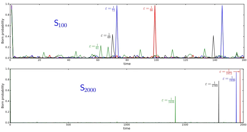
4.4 Monte Carlo simulation of dominant evolutions
Figure 2 shows several dominant evolutions for the standard representation of the groupsS100and S2000. Each graph represents the time dependencies of the Born probabilities for the dominant evolu-tions between four randomly generated pairs of natural vectors. The dominant evoluevolu-tions are marked by labeling their peaks with their base energies: ε ∈ 611,691,721,981andε ∈ 14161 ,17891 ,19391 ,19721
Figure 2.Dominant evolutions between randomly generated states. Born probability vs time
5 Summary
1. A constructive version of the quantum formalism can be formulated in terms of projections of permutations of finite sets onto invariant subspaces.
2. The quantum randomness is a consequence of the fundamental impossibility of tracing the individuality of indistinguishable entities in their evolution.
3. The natural number systems for the quantum formalism are the cyclotomic fields and the field of complex numbers is just their non-constructive metric completion.
4. The observable behavior of a quantum system is determined by the dominants among all possi-ble quantum evolutions.
5. The principle of least action is a continuum approximation of the principle of selection of the most probable trajectories.
References
[1] A.M. Gleason, Indiana Univ. Math. J.6, 885–893 (1957) [2] M. Van Raamsdonk, Gen. Rel. Grav.42, 2323–2329 (2010) [3] J. Maldacena and L. Susskind, Fortschr. Phys.61781–811 (2013) [4] C. Cao, S.M. Carroll, and S. Michalakis, Phys. Rev. D95, 024031 (2017) [5] V.V. Kornyak, EPJ Web of Conferences108, 01007 (2016)
[6] V.V. Kornyak, Mathematical Modelling and Geometry3, No 1, 1–24 (2015) [7] V.V. Kornyak, Phys. Part. Nucl.44, No 1, 47–91 (2013)
[8] R. Solomon, Bull. Amer. Math. Soc. (N.S.)38, No 3, 315–352 (2001)