Marte, Michael (2002): Models and Algorithms for School Timetabling: A Constraint-Programming Approach. Dissertation, LMU München: Fakultät für Mathematik, Informatik und Statistik

(1)

Models and Algorithms for

School Timetabling –

A Constraint-Programming Approach

Dissertation

an der Fakult¨at f¨ur Mathematik, Informatik und Statistik

der Ludwig-Maximilians-Universit ¨at M¨unchen

von

Michael Marte

(2)

(3)

Abstract

In constraint programming [JM94, Wal96, FA97, MS98], combinatorial prob-lems are specified declaratively in terms of constraints. Constraints are relations over problem variables that define the space of solutions by specifying restrictions on the values that the variables may take simultaneously. To solve problems stated in terms of constraints, the constraint programmer typically combines chrono-logical backtracking with constraint propagation that identifies infeasible value combinations and prunes the search space accordingly.

In recent years, constraint programming has emerged as a key technology for combinatorial optimization in industrial applications. In this success, global con-straints have been playing a vital role. Global concon-straints [AB93] are carefully designed abstractions that, in a concise and natural way, allow to model problems that arise in different fields of application. For example, the alldiffconstraint [R´eg94] allows to state that variables must take pairwise distinct values; it has numerous applications in timetabling and scheduling.

In school timetabling, we are required to schedule a given set of meetings between students and teachers s.t. the resulting timetables are feasible and accept-able to all people involved. Since schools differ in their educational policies, the school-timetabling problem occurs in several variations. Nevertheless, a set of en-tities and constraints among them exist that are common to these variations. This common core still gives rise to NP-complete combinatorial problems.

(4)

(5)

Acknowledgments

Franc¸ois Bry introduced me to logic programming and artificial intelligence and supervised this thesis.

Thom Fr¨uhwirth and Slim Abdennadher introduced me to constraint-logic programming and encouraged me to get involved in automated timetabling.

Klaus Schulz promptly agreed to review my work.

From 1999 to 2002, I participated in and was financed by the SIL graduate col-lege (Graduiertenkolleg

”Sprache, Information und Logik“) which in turn was fi-nanced by the DFG (Deutsche Forschungsgemeinschaft, German Research Coun-cil).

I am grateful to Mehmet Dincbas for his invitation to COSYTEC in Paris. The stay at Paris was supported by the BFHZ (Bayerisch-Franz¨osisches Hochschul-zentrum – Centre de Coop´eration Universitaire Franco-Bavarois).

There were fruitful discussions on constraint programming and automated school timetabling with Abderrahmane Aggoun, Nicolas Beldiceanu, Helmut Si-monis, Hana Rudova, and Elias Oliveira.

Norbert Eisinger and Ralph Matthes did some proof reading and made useful suggestions.

Mats Carlsson, the maintainer of SICStus Prolog, contributed with reliable technical support.

Tim Geisler and Sven Panne answered a lot of Haskell-related questions. Martin Josko administered the Condor installation.

Ellen Lilge always was a helping hand in administrative issues.

Last but not least, this project is essentially based on the cooperation with the timetable makers Claus Schmalhofer, Erwin Appenzeller, B¨arbel Kurtz, and Karl-Heinz Auktor.

(6)

(7)

Chapter 1 Introduction

In school timetabling, we are required to schedule a given set of meetings between students and teachers s.t. the resulting timetables are feasible and acceptable to all people involved. Since schools differ in their educational policies, the school-timetabling problem occurs in several variations. Nevertheless, a set of entities and constraints among them exist that are common to these variations. This thesis presents, evaluates, and compares constraint-based solvers for this common core which still gives rise to NP-complete combinatorial problems [EIS76]1.

1.1 School Timetabling

Timetables are ubiquitous in daily life. For example, timetables substantially con-trol the operation of educational institutions, health-care institutions, and public transport systems. Collins Concise Dictionary (4th edition) defines a timetable as a “table of events arranged according to the time when they take place”. Timeta-bles always have to meet domain-specific requirements.

Willemen [Wil02] defines educational timetabling as the “sub-class of time-tabling for which the events take place at educational institutions”. Events include lessons and lectures which occur in class-teacher timetabling and course time-tabling, respectively. We refer to Schaerf [Sch95, Sch99] and Bardadym [Bar96] for well-known reviews of research in automated educational timetabling.

Educational systems differ from country to country and, within a given edu-cational system, education differs from one level of the system to the other. In consequence, different views evolved on how to characterize the categories of educational timetabling. We adopt the view of Carter & Laporte [CL98] who con-sider class-teacher and course timetabling to occur at prototypical high schools

(12)

and universities, respectively, which they regard as opposite extreme points on the continuum of real-world educational institutions.

At the prototypical high school, timetabling is based on classes which result from grouping students with a common program. As only a few programs are of-fered, the number of classes is low. Timetables must not contain conflicts, need to be compact, and have to satisfy various other constraints on the spread and se-quencing of lessons. Since each class has its own classroom, time-slot assignment and room allocation do not interact except for lessons that require science labs, craft rooms, or sports facilities. All rooms and facilities are situated in the same location and hence traveling times are negligible.

In contrast, the prototypical university allows for assembling individual pro-grams. This freedom of choice may render individual timetables without conflicts impossible even though compactness is not an issue. To meet the students’ choices as far as possible, timetable makers try to minimize the number of conflicts. Time-tabling is complicated by room allocation and section assignment. Time-slot as-signment interacts with room allocation because room sizes and requirements of equipment have to be taken into account. Moreover, since rooms and facilities are situated in different locations, traveling times need consideration. The problem of

section assignment arises whenever a course has to be divided for practical

rea-sons. As lectures of different sections may be scheduled independently, the way of sectioning affects timetabling.

(13)

1.2. Constraint Programming 3

1.2 Constraint Programming

In constraint programming (CP) [JM94, Wal96, FA97, MS98], combinatorial problems are specified declaratively in terms of constraints. Constraints are re-lations over variables that define the space of solutions by specifying restrictions on the values that the variables may take simultaneously. To give an example rel-evant to timetabling, the so-calledalldiffconstraint [R´eg94, vH01] takes a set of variables and requires the variables to take pairwise distinct values. As the pro-cess of expressing a given problem in terms of variables and constraints over them is widely perceived as a process of modeling, its outcome is called a constraint

model in this thesis. Note that a constraint model does not contain any information

on how to solve the problem it encodes. The term of declarative modeling refers to this absence of control information.

To solve a combinatorial problem stated in terms of constraints, the constraint programmer usually employs a search procedure based on chronological back-tracking. Driven by branching strategies, chronological backtracking [BV92] un-folds the search space in a depth-first manner. Search nodes represent partial as-signments to decision variables. If a partial assignment cannot be extended with-out violating constraints, chronological backtracking returns to the most recent search node that has a subtree left to expand and explores an alternative. The ef-ficiency of chronological backtracking essentially depends on the quality of the branching strategies.

To reduce the search effort, chronological backtracking is combined with con-straint propagation. From a given problem, concon-straint propagation infers primi-tive constraints like ’variable x must not take value a’ which are used to prune the search space. Typically, constraint propagation and search are integrated tightly: Constraint propagation is invoked after every commitment, domain wipe-outs trig-ger immediate backtracking, and dynamic branching strategies take domain sizes into account. This way constraints take an active role in problem solving.

Typically, constraint propagation is performed by specialized software mod-ules which are called constraint solvers2. Constraint solvers exist independent of each other, they communicate over variable domains only, and when a con-straint solver is applied to a concon-straint, it is not supplied any information except for the constraint itself and the state of its variables. This modular design facili-tates a plug-and-play approach to problem solving, potentially leads to problem solvers that can be adapted to new requirements easily, and allows for embedding application-specific constraint solvers.

When designing a suitable problem solver, the constraint programmer has to

2_{Constraint solvers are sometimes called constraint propagators. In fact, the terms constraint}

(14)

explore a multi-dimensional design space. A problem solver is determined by the choice of a search procedure, of branching strategies, of constraint solvers, and of how to express a given problem in terms of constraints. Due to the sheer number of combinations, only a small part of the design space can be explored. If standard procedures do not apply, expertise from the field of application is likely to be a good guide in this search. In his search, the designer has to address theoretical as well as operational issues. Theoretical issues include correctness3(soundness) and completeness4. Operational issues include running time, memory consump-tion, and reliability in terms of problem-solving capabilities. Completeness may be traded for efficiency and reliability: Frequently, sacrificing solutions by impos-ing additional constraints after careful consideration simplifies the search because, in effect, the search space is reduced. The clarification of operational issues usu-ally requires empirical investigation.

In recent years, constraint programming has emerged as a key technology for combinatorial optimization in industrial applications. Three factors have been de-cisive: the introduction of global constraints, redundant modeling, and the avail-ability of powerful constraint-programming tools (e.g. CHIP5, ECLiPSe6, SICStus Prolog7, ILOG Solver8, Mozart9, CHR [FA97, Fr¨u98]).

Global constraints [AB93] are carefully designed abstractions that, in a

con-cise and natural way, allow to model combinatorial problems that arise in different fields of application. Thealldiffconstraint [Rég94, vH01] mentioned earlier is a prominent representative of global constraints; it has numerous applications in timetabling and scheduling. Global constraints are important because they allow for concise and elegant constraint models as well as for efficient and effective propagation based on rich semantic properties (e.g. [Nui94, Rég94, Rég96, RP97, BP97, PB98, Bap98, Pug98, FLM99, BPN99, MT00, DPPH00, BC01, BK01]).

Redundant modeling [CLW96] refers to the extension of constraint models

with redundant constraints. A constraint is called redundant wrt. a given problem if the problem implies the constraint (i.e. every solution to the problem satisfies the constraint) but does not state it explicitely. Redundant modeling is well known for its potential operational benefits. It can be considered as a kind of constraint prop-agation performed prior to search that results in constraints that are themselves subject to propagation during search.

3_{A problem solver is called correct iff every assignment it outputs is a solution.}

4_{A problem solver is called complete iff, in a finite number steps, it either generates a solution}

or proves that no solution exists.

5_{http://www.cosytec.com} 6_{http://www.icparc.ic.ac.uk} 7_{http://www.sics.se}

8_{http://www.ilog.com}

(15)

1.3. Outline of Thesis 5

For detailed introductions to constraint programming, we refer to the text-books by Tsang [Tsa93], Fr¨uhwirth & Abdennadher [FA97], and Marriott & Stuckey [MS98].

1.3 Outline of Thesis

Research in automated school timetabling can be traced back to the 1960s [Jun86]. During the last decade, efforts concentrated on local search methods such as simulated annealing, tabu search, and genetic algorithms (e.g. [Sch96a, DS97, CDM98, CP01]). Constraint-programming technology has been applied to univer-sity course timetabling (e.g. [GJBP96, HW96, GM99, AM00]) but its suitability for school timetabling has not yet been investigated.

In the first place, this thesis proposes to model the common core of school-timetabling problems by means of global constraints. The presentation continues with a series of operational enhancements to the resulting problem solver which are grounded on the track parallelization problem (TPP). A TPP is specified by a set of task sets which are called tracks. The problem of solving a TPP consists in scheduling the tasks s.t. the tracks are processed in parallel. We show how to expose redundant TPPs in school timetabling and we investigate two ways of TPP propagation: On the one hand, we utilize TPPs to down-size our constraint models. On the other hand, we propagate TPPs to prune the search space. To this end, we introduce thetppconstraint along with a suitable constraint solver for modeling and solving TPPs in a finite-domain constraint-programming framework10. More-over, we propose to reduce the search space by imposing non-redundant TPPs in a systematic way. In summary, this thesis emphasizes modeling aspects. Search procedures and branching strategies are not subject to systematic study.

To investigate our problem solvers’ behavior, we performed a large-scale com-putational study. The top priority in experimental design was to obtain results that are practically relevant and that allow for statistical inference. To this end, the problems have been generated from detailed models of ten representative schools and the sample sizes have been chosen accordingly – for each school, our problem set contains 1000 problems. The school models describe the programs offered to the students, the facilities, the teacher population, the student population, and var-ious requirements imposed by the school management. Our timetabling engine es-sentially embeds network-flow techniques [R´eg94, R´eg96] and value sweep prun-ing [BC01] into chronological backtrackprun-ing. It comprises about 1500 lines of code and has been built on top of a finite-domain constraint system [COC97] which it-self is part of the constraint-logic programming environment SICStus Prolog 3.9.0

10_{In finite-domain constraint programming, we deal with finite-domain constraints defined}

(16)

[Int02]. The experiment was performed on a Linux workstation cluster by means of the high-throughput computing software Condor [Con02].

To facilitate the computational study of problem solvers for school time-tabling, a comprehensive simulation environment has been developed. This soft-ware package contains a problem generator, the school models, and various tools to visualize and analyze problems and solutions. The package has been imple-mented using the state-of-the-art functional programming language Haskell (e.g. [PJH99, Tho99]) and comprises about 10000 lines of code. The school models account for about 2700 lines of code.

This thesis is organized as follows. Chapter 2 introduces to school timetabling. Chapter 3 deals with track parallelization: it introduces the TPP and proposes the tpp constraint along with a suitable solver for modeling and solving TPPs in a finite-domain programming framework. Chapter 4 presents constraint-based solvers for school timetabling, shows how to infer and exploit TPPs in this setting, and presents our computational study of solver behavior. Chapter 5 sum-marizes, discusses the contribution of this thesis wrt. timetabling in general, and closes with perspectives for future work. Appendix A presents a new method for proving confluence in a modular way and applies this method to the TPP solver.

1.4 Publications

The work presented in this thesis was outlined at the 3rd International Conference on the Practice and Theory of Automated Timetabling (PATAT-2000) [Mar00]. Thetpp constraint and its solver (cf. Chapter 3) were presented at the 5th Work-shop on Models and Algorithms for Planning and Scheduling Problems (MAPSP-2001) [Mar01a] and at the Doctoral Programme of the 7th International Confer-ence on Principles and Practice of Constraint Programming (CP-2001) [Mar01b]. The method for proving confluence in a modular way (cf. Appendix A) was pre-sented at the 4th International Workshop on Frontiers of Combining Systems (FroCoS-2002) [Mar02].

1.5 Reduction Systems

A reduction system is a pair(A,→)where the reduction→is a binary relation on the set A, i.e.→⊆A×A. Reduction systems will be used throughout this thesis to

(17)

1.5. Reduction Systems 7

Describing algorithms with reduction systems has some advantages over using procedural programs:

• Reduction systems are more expressive than procedural programs because non-determinism can be modeled explicitely. So we are not required to com-mit to a specific execution order in case there are alternatives.

• Freed from the need to fix an execution order, we can concentrate on the essential algorithmic ideas. There is no need to worry about operational issues like which execution order will perform best in some sense or another.

• If we give a non-deterministic reduction system, every result about its com-putations (like correctness and termination) will apply a fortiori to every of its deterministic implementations.

• We can study the effects of non-deterministic choices: Is there a uniquely determined result for every input? If this is the case for a given reduction system, then its deterministic implementations will have one and the same functionality.

The theory of reduction systems has many results to answer questions on termina-tion and on the effects of non-deterministic choices (for example, see Newman’s Lemma below).

When talking about reductions systems, we will make use of the concepts and the notation introduced in the following (cf. [BN98]):

Definition 1.1. Let(A,→)be a reduction system.

• It is common practice to write a→b instead of(a,b)∈→.

• →=_, _→+_{, and} _→∗ _{denote the reflexive closure, the transitive closure, and} the reflexive, transitive closure of→, respectively.

• We say that y is a direct successor to x iff x→y.

We say that y is a successor to x iff x→+y.

• x is called reducible iff∃y.x→y.

x is called in normal form (irreducible) iff it is not reducible.

y is called a normal form of x iff x→∗y and y is in normal form.

If x has a uniquely determined normal form, the latter is denoted by x↓.

• x,y∈A are called joinable iff∃z.x→∗z←∗y, in which case we write x↓y.

→is called locally confluent iff y←x→z implies y↓z.

(18)

• →is called terminating iff there is no infinite, descending chain a0→a1→

··· of transitions.

• →is called convergent iff it is terminating and confluent.

The following Lemma follows easily from the definition of convergence.

Lemma 1.1. Let (A,→) be a reduction system. If → is convergent, then each a∈A has a uniquely determined normal form.

This Lemma may free us from worrying about whether the non-determinism that is inherent in a certain reduction system allows for computations that produce different results for the same input. With a convergent reduction system, whatever path of computation is actually taken for a given input, the result is uniquely de-termined. In other words, if→is a convergent reduction on some set A, then the reduction{(a,a↓): a∈A}is a function on A.

The following statement provides a tool for proving confluence via local con-fluence; it is called Newman’s Lemma. See [BN98] for a proof.

Lemma 1.2. A terminating reduction is confluent if it is locally confluent.

1.6 Constraint Satisfaction

To faciliate the application of constraint technology to a school-timetabling prob-lem, we have to translate the high-level problem description (in terms of teachers, students, facilities, and meetings) into a so-called constraint satisfaction problem (CSP). A CSP is stated in terms of constraints over variables with domains and to find a solution requires to choose a value from each variable’s domain s.t. the resulting value assignment satisfies all constraints.

The usual way to describe a CSP is to give a triple(X,δ,C)with a set of vari-ables X , a set of constraints C over X , and a total functionδon X that associates each variable with its domain. Another way to specify a CSP is to give a hyper-graph with variables as nodes and constraints as hyperarcs. Such a hyper-graph is called a constraint network.

When talking abount constraint satisfaction and constraint solving, we will use the concepts and the notation introduced in the following:

Definition 1.2. Let P= (X,δ,C)be a CSP.

• δis called a value assignment iff|δ(x)|=1 for all x∈X .

(19)

1.7. Constraint Solving 9

• P is called ground iffδis a value assignment.

• P is called failed iff some x∈X exists withδ(x) = /0.

• A domain functionσon X is called a solution to P iff σis a value assign-ment, xσ∈δ(x)for all x∈X , andσsatisfies all constraints c∈C.

• sol(P)denotes the set of solutions to P.

• If Q is a CSP, too, then P and Q are called equivalent iff sol(P) =sol(Q), in which case we write P≡Q.

• If D is a set of constraints over X , then P⊕D denotes(X,δ,C∪D).

• A constraint c over X is called redundant wrt. P iff c∈/ C and sol(P)⊆

sol(P⊕ {c}).

So a constraint is called redundant wrt. a given problem if every solution to the problem satisfies the constraint though the problem does not state the constraint explicitely.

The following statement about adding constraints follows easily from the properties of solutions:

Lemma 1.3. Let P be a CSP with variables X and let C be a set of constraints over X . P≡P⊕C holds iff P≡P⊕ {c}for all c∈C.

We will consider finite CSPs with integer domains only and use the abbrevia-tion FCSP to denote such problems. If a and b are integers, we will write[a,b]to denote the set of integers greater than or equal to a and smaller than or equal to b, as usual.

1.7 Constraint Solving

In this thesis, constraint solvers will be described through non-deterministic re-duction systems. As explained in Section 1.5, this way of specifying constraint solvers has a number of advantages over giving procedural programs: We may concentrate on the essential algorithmic ideas without bothering about operational issues, our results about computations will apply to every deterministic implemen-tation, and there is a variety of technical means to study questions on confluence. To provide a framework for defining constraint solvers, our next step is to define the FCSP transformer→FDas

(20)

iff X1=X0, C1=C0,δ1=δ0, andδ1(x)⊆δ0(x)for all x∈X0.

The resulting reduction system captures three important aspects of finite-domain constraint solving as we find it implemented in today’s constraint-programming systems: Constraint solvers reduce the search space by domain re-ductions, they cooperate by communicating their conclusions, and this process will not stop until no transition applies. Further aspects of constraint solving like correctness will be considered later on.

The possibility of adding variables and constraints has not been provided for because we will not consider computations where constraint solvers add new con-straints except for such that can be expressed in terms of domain reductions.

It is easy to see that→FD is transitive and convergent. Because of

transitiv-ity, it is not necessary to distinguish successors, that are reached by one or more reduction steps, from direct successors.

The following monotonicity properties of domain bounds and solutions sets are immediate:

Corollary 1.1. Let P0and P1be FCSPs with P0→FDP1.

1. Lower (Upper) bounds of domains grow (shrink) monotonically, i.e.

minδ0(x)≤minδ1(x)≤maxδ1(x)≤maxδ0(x)

for all x∈X where δ0 and δ1 denote the domain functions of P0 and P1,

respectively.

2. Solution sets shrink monotonically, i.e. sol(P0)⊇sol(P1).

We continue by considering those subsets of →FD that preserve solutions: We

define the reduction→Cas

{(P0,P1)∈→FD: P0≡P1}

and call a subset of→FD correct iff it is contained in→C. Clearly,→Cis correct

itself and every correct reduction is terminating.

If a correct reduction reliably detects variable assignments that violate a given constraint, then we call the reduction a solver for this particular constraint:

Definition 1.3. Let c be a constraint and let→⊆→FD.→is called a solver for c iff

(21)

1.7. Constraint Solving 11

The requirement of correctness restricts the scope of the preceding definition to those subsets of→FD that perform deduction by adding redundant constraints

in terms of domain reductions. Returning a failed problem signals the embedding search procedure11 that a constraint violation has occured, causes it to reject the variable assignment, and to look for another one.

By requiring that violated constraints do not go unnoticed, we can be sure that any variable assignment returned by any embedding search procedure is a solution. Nevertheless, one might object that the definition is not quite complete because it does not impose any bound on time complexity though a decent con-straint solver is usually required to run in polynomial time12. However, such a definition would rule out generic constraint solvers with exponential worst case complexity that apply to any constraint but are not practical unless the constraint to be propagated has only a few variables with small domains. Such a constraint solver (e.g. [BR99]) is useful if a specialized constraint solver is not available and developing one does not pay off because the run times exhibited by the generic constraint solver are reasonable.

The preceding definition might be objected to for another reason: It allows for problems solvers that implement a pure generate & test approach. This contradicts the spirit of constraint programming whereby constraints should take an active role in the problem-solving process as early as possible because search becomes easier the more values are pruned and the earlier this happens13. The definition does not make any requirement in this direction because what kind of reasoning should be performed really depends on the application. If there is any need to specify the reasoning power of a constraint solver, there are established ways to do this like asserting the maintenance of interval or domain consistency [VSD98]. Note that there are two ways to employ reductions that are correct but that do not solve a constraint or a class of constraints in the sense of the preceding definition. Such reductions can be used to propagate redundant constraints or to provide additional pruning.

It remains to clarify how to combine constraint solvers defined as reductions. If

→1,...,→nare constraint solvers, then there are two immediate ways to combine

11_{Constraint solvers on their own are not able to solve problems. A given problem may have}

many solutions and committing to one of them is beyond deduction. So we find constraint solvers embedded into search procedures like chronological backtracking.

12_{With regard to the definition of constraint solvers in terms of reductions, to run in polynomial}

time means that every path of computation ending in a normal form can be traversed in polynomial time. This is not possible unless every transition can be carried out in polynomial time.

13_{Of course, the overall efficiency of a problem solver depends on the nature of the problems it}

(22)

them: Either we use their union or we use

1≤i≤n

{(P,Q): P is a FCSP, Q=P, and Q is a normal form of P wrt.→i}. The latter method comes closer to what actually happens in today’s constraint-programming systems: When a variable domain is reduced (either by constraint propagation or by the search procedure committing to a choice14), then the con-straints containing the variable are determined and the corresponding constraint solvers are scheduled for invocation. When a constraint solver is eventually ap-plied to a constraint, then the former is expected to reduce the search space in-stantaneously and as far as it is able to do so. This way the constraint does not require further consideration until it has its wake-up conditions satisfied again.

(23)

Chapter 2 School Timetabling

Besides NP-completeness, there is another fundamental issue in school time-tabling, namely the diversity in problem settings. Even schools of the same type may differ with regard to the requirements of their timetables. In face of this diver-sity, which constraints does a timetabling algorithm need to handle to be widely applicable? It is clear that a timetabling algorithm will not be very useful unless it can handle the frequent constraints. But which constraints occur frequently? This question is studied in Section 2.1 which, at the same time, introduces the reader to school timetabling.

Section 2.2 continues the presentation with introducing a special class of schools – namely German secondary schools of the Gymnasium type. Among other things, their timetabling problems are characterized and the process of man-ual timetabling is explained. The treatment is very detailed to enable the reader to assess the scope of the results presented in Chapter 4 where the operational prop-erties of constraint-based solvers for school timetabling are studied on problems from schools of the Gymnasium type.

Research in automated school timetabling can be traced back to the 1960s and, during the last decade, efforts concentrated on greedy algorithms and on local search methods. Several case studies have been performed and some promising results have been obtained. Section 2.3 closes the chapter with a review of these more recent approaches.

2.1 The Core of School-Timetabling Problems

(24)

Mon Tue Wed Thu Fri 1

2 3 4 5 6

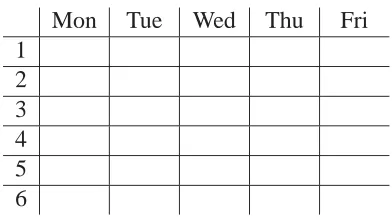
Figure 2.1: A typical time grid with five days and six time slots a day

rooms, and meetings of fixed duration) and constraints among them exist that are common to these variations. This section details on the core’s composition from the author’s point of view (c.f. Figure 2.2) which is based on a survey of more recent publications [Cos94, Sch96b, Sch96a, DS97, CDM98, FCMR99, KYN99, BK01, CP01], on a survey of commercial timetabling software1(gp-Untis 20012, Lantiv Timetabler 5.03, OROLOGIO 114, SPM 3.15, TABULEX 2002 (6.0)6, Turbo-Planer 20007), and on the author’s own field work.

Meetings are regular events of fixed duration including lessons, consulting hours, and teacher meetings. A meeting is specified in terms of a student set (empty in case of consulting hours and teacher meetings), a non-empty teacher set (usually singleton in case of a lesson), and a non-empty set of suitable rooms. It is understood that a meeting has to be attended by every of its teachers and students and that is has to be held in one of the designated rooms.

We assume that the meetings of a problem are packed into jobs. A job is a set of meetings and we require the jobs of a problem to partition its meeting set. All the meetings of a job have to be identical with regard to their resource requirements. Typically, a job comprises all the lessons of some class in some subject.

Timetabling is based on a rectangular time grid that divides the planning pe-riod into disjoint time intervals of equal duration which are called time slots or simply periods8. Figure 2.1 shows a typical time grid with five days and six time

1_{This survey is based on data sheets, manuals, tutorials, on-line help files, and demo versions}

that were available from the Internet.

2_{Gruber & Petters Software, Austria,}_{http://www.grupet.at} 3_{http://www.lantiv.com}

4_{ANTINOOS Software Applications, Greece,}_{http://www.antinoos.gr} 5_{http://www.stundenplanmanager.de}

6_{ZI SOFT KIEL, Germany,}_{http://www.ziso.de} 7_{Haneke Software, Germany,}_{http://www.haneke.de}

8_{Actually, the term period has at least three different uses in school timetabling: (a) In phrases}

(25)

2.1. The Core of School-Timetabling Problems 15

slots a day. A time slot can be addressed by its day and its index (contained in the left-most column of the time grid displayed in Figure 2.1). The amount of time represented by a time slot usually equals the amount of time required to give a les-son though we do not impose any restriction on the granularity of time. Meeting durations and start times are specified in terms of time slots.

As start times and rooms are not fixed in advance of planning (the exception proves the rule), the process of timetabling involves scheduling and resource al-location with the aim to create a timetable for each student and each teacher. As a by-product, timetables for each room are obtained. The space of solutions is restricted by the following constraints:

1. Resource capacities: Resources (students, teachers, and rooms) must not be double-booked.

2. Restrictions on availability: Resources may be unavailable for given pe-riods of time9. Such restrictions are expressed through sets of time slots (so-called time frames). Periods of unavailability will also be referred to as

down times.

3. Couplings: A coupling requires to schedule a given set of jobs in parallel10.

4. Distribution constraints (c.f. Table 2.1):

(a) Lower and upper bounds on daily work load: This type of constraint occurs for students, teachers, student-teacher pairs11, jobs12, and pairs of students and job sets13. It does not occur for rooms. Work load is measured in time slots.

(b) Lower and upper bounds on the number of working days: This type of constraint occurs only for students and teachers.

we specify a certain amount of time; acting as a unit of measure, the term period refers to the duration of time slots.

9_{Restrictions on availability may result from the sharing of teachers and facilities among}

sev-eral schools.

10_{Couplings are essentially a consequence of study options (cf. Section 2.2 and Section 4.3).}

Timetabling may be complicated considerably by couplings due to simultaneous resource de-mands. As a rule of thumb, the more study options are offered the more couplings will give a headache to the timetabler.

11_{This way, for each student and for each of its teachers, the daily amount of time spent together}

in class may be bounded.

12_{This way job-specific bounds on the daily amount of teaching may be imposed.}

13_{This way, for each student, the daily amount of time main subjects are taught to the student}

(26)

Bounds on daily work

load

Bounds on the number of working days

Bounds on total idle time

gp-Untis 2001 +/+ +/+ +/+

Lantiv Timetabler 5.0 +/+ -/- +/+

OROLOGIO 11 -/+ -/- +/+

SPM 3.1 +/+ -/+ +/+

TABULEX 2002 (6.0) +/+ +/- -/+

Turbo-Planer 2000 +/+ -/+

+/-[Cos94] -/- -/- -/+

[Sch96b, Sch96a] +/+ -/+ -/+

[DS97] -/+ -/-

-/-[CDM98] -/- -/-

-/-[FCMR99] -/+ -/- -/+

[KYN99] -/+ -/-

-/-[BK01] +/+ -/-

-/-[CP01] -/+ -/+ -/+

Author’s field work +/+ -/+ +/+

Table 2.1:

Survey of the most frequent distribution constraints

stud

ents teac_he rs ro om_s meet ing s couplings re sou rce capa

cities restrictio_ns

on av ail ab ili ty bound

s on daily work load

boundson

the num ber of wo rk in g d ays b o u n d s o n to ta

l id_le

tim_e

(27)

2.2. The GermanGymnasium 17

(c) Lower and upper bounds on total idle time: Timetables may contain time slots that are not occupied by any meeting. Such a time slot in the middle of a day is called idle, a gap, or a hole (in German

Fensterstun-de, FreistunFensterstun-de, HohlstunFensterstun-de, or Springstunde), if there are meetings

scheduled before and after it. The number of idle time slots that occur in a personal timetable is referred to as the person’s total14 idle time.

(Bounds on total idle time occur only for students and teachers.)15

Lower bounds on daily work load and on total idle time have in common that they do not apply to free days. For example, consider a teacher with bounds l and u on her daily work load. For each day of the planning period, the teacher’s timetable has to satisfy the following condition: Either the day is free or at least l and at most u time slots are occupied by meetings of the teacher.

The list actually comprises most constraints on student, teacher, and room timetables that occur in practice. Yet school-timetabling problems differ consid-erably regarding those distribution constraints that directly affect job timetables. These constraints are therefore not included in the common core except for bounds on the number of time slots that may be occupied a day. (Such bounds occur frequently.) Despite this restriction, the common core gives rise to NP-complete combinatorial problems [EIS76]16.

In practice, hard constraints are distinguished from soft constraints. Hard

con-straints are conditions that must be satisfied whereas soft concon-straints may be

vi-olated but should be satisfied as much as possible. By their very nature, resource capacities and restrictions on resource availability occur only as hard constraints. The author’s study showed that couplings occur only as hard constraints and that distribution constraints occur mainly as soft constraints.17

2.2 The German Gymnasium

In this thesis, the operational properties of constraint-based solvers for school timetabling are studied on problems from German secondary schools of the

Gym-nasium type. This type of school offers nine grades of academically orientated

14_{Rarely there are bounds on daily idle time.}

15_{The publications that were subject to review talk about the need to minimize the number of}

idle time slots but do not give any bounds. A close look into the models revealed that idle time slots are not allowed at all and hence that the upper bounds equal zero.

16_{See also [GJ79], problem SS19.}

17_{With the commercial timetabling packages, the definition of a problem is carried out in two}

(28)

education (numbered from five through thirteen). This section characterizes the German Gymnasium and its timetabling problems and it describes the processes of problem specification and manual timetabling.

2.2.1 Educational Programs

Each school offers a specific set of educational programs and the higher the grade, the higher the number of programs. Foreign-language education starts right in the fifth grade and, usually, English is taught as first foreign-language but there may be options. Then the number of study options increases in three steps:

1. From the seventh grade, a second foreign language is introduced and there may be school-specific options like, for example, either French or Latin.

2. From the ninth grade, education may diversify further because several study directions may be offered. Official regulations [App98] define six study directions: Humanities, Modern Languages, Music and Arts, Natural Sci-ences, Economics, and Social Sciences. In Humanities and Modern Lan-guages, a third foreign language is introduced and, again, there may be school-specific options.

3. For the grades twelve and thirteen (in German Kollegstufe), the study direc-tions of the previous grades are discontinued in favor of a system where each study direction is based on a pair of advanced-level courses (in German

Lei-stungskurse). Official regulations [Kol97] (updated yearly) define which

base pairs are admissible (140 base pairs were admissible in 1997) and, for each base pair, define constraints on the individual choice of foundation

courses (in German Grundkurse). In practice, about ten to twenty study

di-rections are implemented. The choice of study didi-rections varies from school to school and from year to year. It is determined by what the school man-agement offers and by what the students demand for.

The choice of a study direction does not always determine a program completely because many study directions, in particular those of the final grades, may offer options. Hence, to fix their programs, students may have to meet further decisions such as the students of Modern Languages who may have to choose a third foreign language from a given set of alternatives.

(29)

denominations. Catholic and Protestant students receive specific religious educa-tion18 while members of other denominations have to undergo ethical education. Consequently, if two students differ in religious denomination, they have different programs unless both of them receive ethical education.

From the fifth through the eleventh grade, a Gymnasium more or less resem-bles the prototypical high school (c.f. Section 1.1). There are classes with fixed classrooms though, frequently, heterogeneous classes with students of different programs (boys and girls, Catholics and Protestants, and students of different study directions) cannot be avoided. Subjects that are common to all programs occurring in a class are taught to the class as a whole. For education in program-specific subjects, classes are split and students from different classes are united. In combination with tight time frames (except for the eleventh grade, student timeta-bles usually must not contain idle time), this procedure leads to requests for par-allel education of several groups that complicate timetabling considerably due to simultaneous resource demands (cf. Section 4.3).

In the final grades, a Gymnasium more or less resembles the prototypical uni-versity. Students with identical programs are rare, there are no classes, and the student timetables have to satisfy moderate compactness constraints.

2.2.2 The Problem Specification Process

The specification of the next school year’s timetabling problem lies in the hands of the headmaster. When specifying the problem, the headmaster has to keep to offi-cial regulations [App98] that for each grade, study direction, and subject specify the subject matter and the weekly number of teaching periods. In particular, those regulations restrict the possibilities for joint education of students from different study directions.

The specification process results in a set of so-called modules. A module re-quires to split a given set of students into a given number of groups of similar size and to educate each group for a given number of periods in a given subject. To this end, each module is assigned a set of suitable rooms and each of its groups is assigned a suitable teacher. We distinguish intra-class from inter-class modules. The students of an intra-class module all stem from the same class while an

inter-class module joins students from at least two inter-classes. To translate a module into

a set of jobs (c.f. Section 2.1), we need to fix the group members and the meeting durations.

18_{Parents of a Catholic or Protestant student may require that their child undergoes ethical}

(30)

2.2.3 The Effects of Study Options

To illustrate the effects of study options on timetabling data, two examples will be given. But first it is necessary to describe the school that the examples stem from: In the fifth grade, all students start to learn English. From the seventh grade, the foreign-language curriculum has to be extended with either Latin or French. Thus there are two programs: English-Latin (EL) and English-French (EF). From the ninth grade, three study directions are offered: Modern Languages (ML), Social Sciences (SOC), and Natural Sciences (NAT). Latin is a prerequisite for ML and ML students are taught French as third foreign language. In summary, there are five programs: ML-ELF, SOC-EL, SOC-EF, NAT-EL, and NAT-EF.

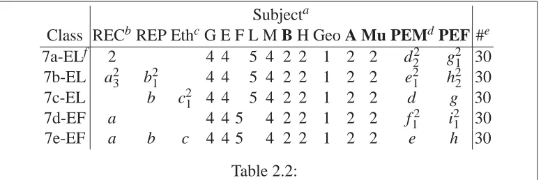
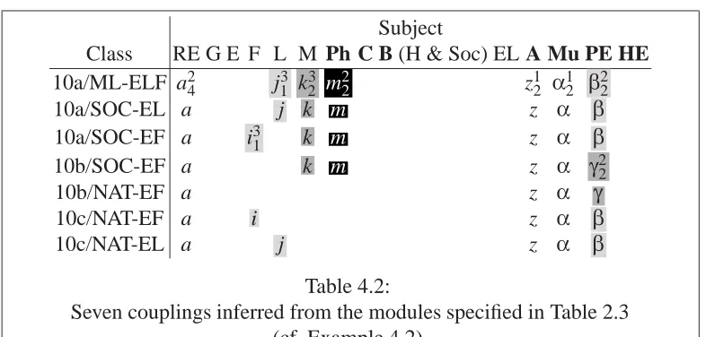
Example 2.1. Table 2.2 defines the seventh grade of a Gymnasium timetabling

problem in terms of its modules. For each subject, there is a column and, for each class, there is a row. There are five classes (7a through 7e) all of which are homogeneous wrt. the foreign-language curriculum: 7a, 7b, and 7c are EL classes while 7d and 7e are EF classes.

Depending on the corresponding subject, a table field either relates to the cor-responding class as a whole or only to a part of it. For example, the fields in religious education relate to the respective denominational groups only. With this policy, the meaning of the table fields is defined as follows:

• If the field(c,s)is empty, then there is no requirement to teach the subject

s to any student of the class c.

• Numbers specify intra-class modules: If the field (c,s)contains n, then n time slots must be reserved weekly for teaching the subject s to the respec-tive students of the class c. There is no requirement for joint education with students of other classes.

• Letters uniquely identify inter-class modules: If the field(c,s)contains m, then the respective students of the class c are to be educated jointly with the respective students of those classes for which the column s holds m, too.

• Subscripts and superscripts give additional information on the respective inter-class modules: The subscript specifies the required number of groups and the superscript specifies the number of time slots that need to be re-served weekly. For each inter-class module, there is exactly one field (the left- and/or top-most one) that gives this information.

(31)

Subjecta

Class RECbREP EthcG E F L M B H Geo A Mu PEMdPEF #e

7a-ELf 2 4 4 5 4 2 2 1 2 2 d2₂ g2₁ 30

7b-EL a2₃ b2₁ 4 4 5 4 2 2 1 2 2 e2₁ h2₂ 30

7c-EL b c2₁ 4 4 5 4 2 2 1 2 2 d g 30

7d-EF a 4 4 5 4 2 2 1 2 2 f₁2 i2₁ 30

7e-EF a b c 4 4 5 4 2 2 1 2 2 e h 30

Table 2.2:

The seventh grade of a Gymnasium timetabling problem in terms of its modules (cf. Example 2.1).

a_{Subject Codes: REC/REP = Religious Education for Catholics/Protestants, Eth = Ethics, G} = German, E = English, F = French, L = Latin, M = Mathematics, B = Biology, H = History, Geo = Geography, A = Art, Mu = Music, PEM/PEF = Physical Education for Boys/Girls. If a subject code is printed in bold face, a science lab, a craft room, or some other special facility is required.

b_{By default, all Catholic students attend REC and all Protestant students attend REP.} c_{All students that are neither Catholic nor Protestant attend Eth. Furthermore, parents of a} Catholic or Protestant child may require that their child attends Eth instead of REC or REP.

d_{In this school, the sexes are segregated in physical education.}

e_{For each class, this column gives the total number of teaching periods per week.}

f_{7a is a pure Catholic class while all the other classes are mixed wrt. religious denomination.}

The composition of the classes has lead to several inter-class modules. For ex-ample, module e specifies a boy group and requires that it has to attend physical education for two periods a week (cf. field (7b-EL, PEM)) while module h speci-fies two girl groups and requires that each of them has to attend physical education for two periods a week (cf. field (7b-EL, PEF)). Both modules arise from sexual segregation in physical education. Module e serves to save a teacher while module

h serves to specify groups of similar size.

Interestingly, the introduction of the second foreign language has not entailed any inter-class modules because it was possible to create classes that are homoge-neous wrt. the foreign-language curriculum.

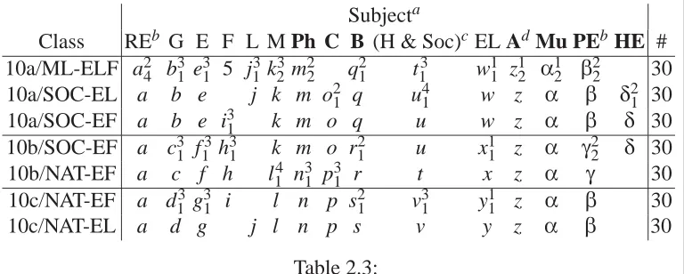
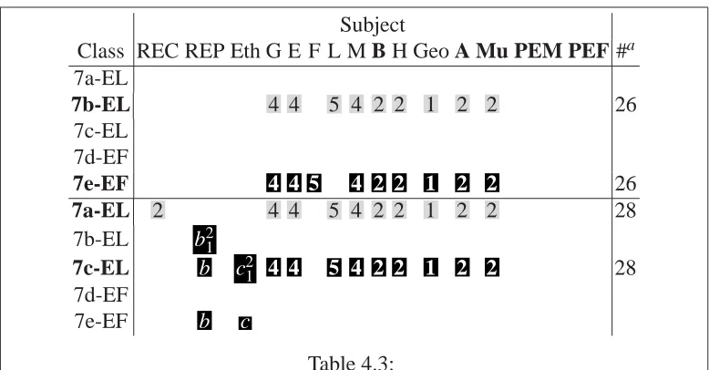
Example 2.2. Table 2.3 defines the tenth grade of a Gymnasium timetabling

(32)

Subjecta

Class REb G E F L M Ph C B (H & Soc)c EL AdMu PEbHE #

10a/ML-ELF a2₄ b3₁ e3₁ 5 j₁3k3₂m2₂ q2₁ t₁3 w1₁ z1₂ α1₂ β2₂ 30

10a/SOC-EL a b e j k m o2₁ q u4₁ w z α β δ2₁ 30

10a/SOC-EF a b e i3₁ k m o q u w z α β δ 30

10b/SOC-EF a c3₁ f₁3h3₁ k m o r2₁ u x1₁ z α γ2₂ δ 30

10b/NAT-EF a c f h l₁4 n3₁ p3₁ r t x z α γ 30

10c/NAT-EF a d₁3g3₁ i l n p s2₁ v3₁ y1₁ z α β 30

10c/NAT-EL a d g j l n p s v y z α β 30

Table 2.3:

The tenth grade of a Gymnasium timetabling problem in terms of its modules (cf. Example 2.2).

a_{In addition to the subject codes introduced in Table 2.2, we use the following subject codes:} RE = Religious Education, Ph = Physics, C = Chemistry, Soc = Social Studies, EL = Economics and Law, PE = Physical Education, HE = Home Economics

b_{For reasons of space, we merged REC, REP, and Eth into RE, and PEM and PEF into PE.} c_{History is taught for two periods a week in the first term and for one period a week in the} second term. Depending on the study direction, Social Studies is taught for one or two periods a week in the first term and for two or three periods a week in the second term.

d_{Students must opt for either Art or Music.}

strange class because its students are not educated jointly except for nine periods a week.)

The way table fields are labeled corresponds to Example 2.1 except for one extension: Letters are used to designate both inter-class and intra-class modules.

We observe two inter-class modules in foreign-language education: Modules

i and j join the French and Latin takers, respectively, of 10a and 10c that learn

(33)

2.2.4 Typical Requirements of Timetables

In the course of timetabling, each lesson (and each other meeting like consulting hours) has to be assigned a start time and a suitable room. As a module specifies a teacher for each of its groups, the assignment of teachers to lessons is fixed in advance of timetabling.

Teacher timetables have to satisfy individual restrictions on availability (like do not schedule any lesson before 9 a.m.), moderate compactness constraints (like at most six periods of idle time a week), individual bounds on daily working time (like not less than two and not more than six periods), and individual bounds on the number of working days (like at least one day off).

Student timetables have to satisfy grade-specific restrictions on student avail-ability: From the fifth through the tenth grade, compact timetables are enforced through tight time frames where the number of acceptable time slots equals the number of teaching periods as prescribed by official regulations. In the final grades, the time frames are loose and, to avoid unacceptable timetables, bounds on daily working time (like at least four and at most eight periods) and bounds on idle time (like at most two periods a day and at most six periods a week) are imposed.

Rooms timetables may have to satisfy room-specific restrictions on availabil-ity, for example, if public sports facilities have to be shared with other schools.

Job timetables have to satisfy job-specific distribution constraints (like at most two teaching periods a day).

2.2.5 Manual Timetabling

Starting out from the headmaster’s problem specification, the timetables are cre-ated by dediccre-ated teachers. In manual timetabling, it is common to proceed in an iterative fashion where each iteration selects and schedules a lesson. Scheduling a lesson requires to choose a room and a time slot s.t. the commitment to the choice will not violate any constraint. (If the school has a lot of rooms, room allocation may be performed after scheduling.) In case no good choice is available for the lesson under consideration, a conflict resolution method is used to free a good time slot by moving and interchanging lessons already scheduled. Both lesson selec-tion and conflict resoluselec-tion are supported by problem specific guidelines. Finally, if there is time left, the timetable is optimized by means of conflict resolution. Due to changes in problem structure, timetables have to be created from scratch every year.

(34)

until a good time slot is available. Consider the following problem: One lesson of English is left to schedule, but the teacher is not available for any of the free time slots. Local repair looks for a good time slot and dispels the lesson occupying it. If there is a good unused time slot for the dispelled lesson, then the lessons are scheduled and local repair finishes. If there is no good unused time slot for the dispelled lesson, local repair iterates in order to schedule the dispelled lesson. As experience shows, human timetable makers can cope with up to ten iterations.

Not only the timetable is subject to change in the course of local repair; the teacher assignment may be changed, too. But since consequences of changing the teacher assignment may be difficult to track and to cope with, such changes come into question only in early stages of timetabling. Furthermore, the headmas-ter, who is the person in charge, must be consulted before changing the teacher assignment.

Neither the next lesson to schedule, nor the next lesson to dispel is chosen arbitrarily because lessons are not equal with respect to number and tightness of constraints. Since the satisfaction of constraints gets harder and harder with the number of free time slots decreasing, it is clever to schedule more constrained lessons first. This strategy diminishes the number of conflicts to resolve in the further course of timetabling. In local repair, if the lesson to dispel can be chosen from a set of candidates, it has proved advantageous to dispel the least constrained lesson. In general, this lesson can be scheduled easier than the more constrained lessons. This strategy diminishes the average number of iterations necessary to resolve a conflict.

Usually, lesson selection is supported by a school-specific, hierarchical les-son selection scheme. Each level of the hierarchy defines a set of lesles-sons which are considered equivalent in terms of constrainedness. The levels are ordered: the higher the level the more constrained the lessons. According to the strategy in-troduced above, timetabling starts with scheduling lessons from the highest level. After placing the most constrained lessons, timetabling continues with the next level, and so on. In general, when scheduling a level’s lessons, the lessons of classes and teachers that only have a few lessons left to schedule are preferred. Again, this strategy avoids expensive conflict resolutions.

2.3 Recent Approaches in Automated School

Time-tabling

(35)

2.3. Recent Approaches in Automated School Timetabling 25

Methods Problems

Reference GAa SAb TSc CPd GrAe HCf artificial real-world

[Cos94] • • 2

[YKYW96] • • • 7

[Sch96b, Sch96a] • • 1 2

[DS97] • • 30

[CDM98] • • • • 3

[FCMR99] • 1

[KYN99] • • • 4

[BK01] • • • •

[CP01] • 1

Table 2.4:

Overview of research in automated school timetabling

a_{Genetic Algorithm} b_{Simulated Annealing} c_{Tabu Search}

d_{Constraint Propagation} e_{Greedy Algorithm}

f_{Hill Climbing}

(e.g. [Sch96a, DS97, CDM98, CP01]). Constraint-programming technology has been used to solve timetabling problems from universities (e.g. [GJBP96, HW96, GM99, AM00]) but the question whether it applies to school timetabling as well is open.

In the following, research is reviewed that has been carried out in the field of automated school timetabling during the past ten years (cf. Table 2.4). For reviews of earlier work on heuristic, mathematical-programming, and graph-theoretical approaches, the reader is refered to the well-known surveys of de Werra [dW85], Junginger [Jun86], and Schaerf [Sch95, Sch99].

(36)

the objective to minimize constraint violations. Then a hill climber is applied in an attempt to resolve the conflicts by moving single lessons. Yoshikawa et al. applied their approach to seven timetabling problems from three Japanese high schools. They characterize their solutions in terms of penalty points but do not describe the underlying objective function. However, they report that the application of SchoolMagic considerably reduced the costs of timetabling for all three schools.

Kaneko et al. [KYN99] improve on [YKYW96] by invoking local repair every time a lesson cannot be scheduled without constraint violations. Their hill climber escapes local optima by moving two lessons simultaneously while accepting mi-nor additional constraint violations. Applying their approach to four timetabling problems from [YKYW96], the authors demonstrate that their improvements ac-tually pay off.

Costa [Cos94] presents a timetabling algorithm based on tabu search. The al-gorithm starts out from a possible inconsistent initial assignment created by a greedy algorithm. In scheduling, the greedy algorithm prefers the lessons with the tightest restrictions on availability and it tries to avoid double-bookings. (Costa notes that it does not pay off to employ stronger methods in initial assignment because this might result in starting points already near to a local optima which are likely to trap tabu search.) In tabu search, the neighborhood is explored by moving single lessons. Costa applied his approach to two high-school timetabling problems from Switzerland. He reports that both problems were solved to full satisfaction.

Schaerf [Sch96b, Sch96a] presents a hybrid approach that interleaves tabu search with randomized hill climbing that allows for sideway moves to explore plateaus. The hybrid generates a random initial assignment and then hill climbing and tabu search take turns for a given number of cycles. Tabu search performs

atomic moves while hill climbing performs double moves. Atomic moves modify

teacher timetables by moving or exchanging lessons. A double move sequences a pair of atomic moves. Hill climbing serves to make “substantial sideway modifi-cations” to escape local optima. Schaerf applied his approach to two timetabling problems from Italian high schools and to one artificial problem. He reports that his algorithm produced conflict-free timetables which were better than timetables created manually or by commercial timetabling software.

(37)

2.3. Recent Approaches in Automated School Timetabling 27

with repair which, in turn, performed better than simulated annealing with relax-ation. All the algorithms produced conflict-free timetables that were better than timetables created manually or by commercial timetabling software.

Fernandes et al. [FCMR99] present a genetic algorithm that starts out from a random initial population and employs genetic repair to speed up evolution. The repair function tries to reduce the number of conflicts by moving lessons. It is guided by a strategy that recommends to move most-constrained lessons first. The algorithm was studied on a problem from a Portuguese high school. It produced a timetable that was conflict-free but worse than a hand-made timetable.

Drexl & Salewski [DS97] compare a randomized greedy algorithm to a genetic algorithm that optimizes scheduling strategies. The greedy algorithm is guided by scheduling strategies (priority rules) which rank alternatives in terms of priority

values. Decisions are met “randomly but according to probabilities which are

pro-portional to priority values”. Thus no alternative is ruled out completely though those with higher probabilities are more likely to be selected. The genetic algo-rithm operates on genes that represent random numbers which are used to drive the greedy algorithm to obtain timetables from genetic information. To test their algo-rithms, Drexl & Salewski generated 30 problems from three classes of tractability (easy, medium, and hard) with 35 lessons on average. The authors report that both approaches yield solutions close to optimality.

Brucker and Knust [BK01] advocate the application of project-scheduling technology to school timetabling. Their proposal is centered around (variants of) the resource-constrained project scheduling problem (RCPSP) where a set of tasks with individual resource demands has to be scheduled within a given time horizon under consideration of precedence constraints, parallelity constraints, and resource availabilities, among others, while minimizing a cost function. For this kind of problem, the authors present a variety of deductive methods and they ex-plain how these methods could be employed in local search (to preprocess the input) and in tree search (to prune the search space after each commitment). The authors do not report any computational results.

Carrasco and Pato [CP01] start out from the observation that the sole quest for good teacher timetables entails bad student timetables and vice versa. In face of two objectives that conflict with each other in optimization, the authors pro-pose a genetic algorithm that searches for pareto-optimal solutions. Carrasco and Pato applied their approach to a timetabling problem from a Portuguese vocational school. They report that the genetic algorithm produced many non-dominated so-lutions that were better than a hand-made timetable.

(38)

and thus their results do not generalize beyond their samples. This common defi-ciency in experimental design has a simple reason: despite 40 years of automated school timetabling, the timetabling community has not yet compiled a suitable problem set. In fact, Costa [Cos94] complains that “it is difficult to judge the value of a given timetable algorithm” because “there are no standard test problems or measures of difficulty”. Schaerf [Sch96b] adds that “the absence of a common definition of the problem and of widely-accepted benchmarks prevents us from comparing with other algorithms”.

(39)

Chapter 3 Track Parallelization

This chapter introduces the track parallelization problem (TPP) and proposes the tppconstraint along with a suitable solver for modeling and solving this kind of scheduling problem in a finite-domain constraint-programming framework.

TPPs play a central role in Chapter 4 which proposes and investigates constraint-based solvers for school timetabling. TPPs are used to down-size the underlying constraint models (by a transformation a priori to search) and to prune the search space (by propagation during search).

This chapter is organized as follows. Section 3.1 introduces the TPP and demonstrates that track parallelization is NP-complete. Section 3.2 introduces the tppconstraint and prepares the grounds for the further treatment. Section 3.3 pro-poses a rule-based solver for tpp constraints, demonstrates its correctness, and gives performance guarantees. Section 3.4 closes the chapter with a survey of re-lated work in operations research.

3.1 The Track Parallelization Problem

A track parallelization problem (TPP) is specified by a set of task sets

T

. The task sets are called tracks . For each task t∈

T

, we are given a set of start times

S(t)and a set of processing times P(t) . The problem of solving a TPP consists in scheduling the tasks s.t. the tracks are processed in parallel. More precisely, for each task t∈

T

, we are required to find a processing interval

[s(t),s(t) +p(t)−1] with s(t)∈S(t)and p(t)∈P(t)s.t.

Marte, Michael (2002): Models and Algorithms for School Timetabling: A Constraint-Programming Approach. Dissertation, LMU München: Fakultät für Mathematik, Informatik und Statistik

Models and Algorithms for

School Timetabling –

A Constraint-Programming Approach

Dissertation

an der Fakult¨at f¨ur Mathematik, Informatik und Statistik

der Ludwig-Maximilians-Universit ¨at M¨unchen

von

Michael Marte

Abstract

Acknowledgments

Contents

Chapter 1

Introduction

1.1

School Timetabling

1.2

Constraint Programming

1.3

Outline of Thesis

1.4

Publications

1.5

Reduction Systems

1.6

Constraint Satisfaction

1.7

Constraint Solving

Chapter 2

School Timetabling

2.1

The Core of School-Timetabling Problems

2.2

The German Gymnasium

2.2.1

Educational Programs

2.2.2

The Problem Specification Process

2.2.3

The Effects of Study Options

2.2.4

Typical Requirements of Timetables

2.2.5

Manual Timetabling

2.3

Recent Approaches in Automated School

Time-tabling

Chapter 3

Track Parallelization

3.1

The Track Parallelization Problem

T

T

T