A Comparative Study and Validation of Kinematic Analysis of Planar Four Bar Mechanism Using MSC Adams

(1)

IJEDR1603129

International Journal of Engineering Development and Research (www.ijedr.org)

786

A Comparative Study and Validation of Kinematic

Analysis of Planar Four Bar Mechanism Using MSC

Adams

Rohit Ramesh Burte1_{, Sachin S. Mestry}2 1_{M.E (Machine Design) Student,}2_{Assistant Professor,}

1, 2_{Department of Mechanical Engineering}

1, 2 _{Finolex Academy of Management and Technology, Ratnagiri-415639, Maharashtra, India}

_______________________________________________________________________________________________

Abstract—The aim of this article is to perform an analysis of a four-bar mechanism and to develop a functional model of mechanism in ADAMS/View software. In the analysis and design of mechanisms, kinematic quantities such as velocities and accelerations are of great engineering importance. Kinematics analysis was performed analytically and graphically. To get values of angular velocity and angular acceleration of individual members of the mechanism at different positions of the crank, a computer program is developed with the help of MATLAB software which performs position, velocity, and acceleration analysis. Also, the graphical analysis is performed using relative velocity method. The modelling and simulation of mechanism is done with the help of ADAMS software for easier evaluation of the results. During that different nature of graph in ADAMS on angle of link, angular velocity of link and angular acceleration verses time in anticlockwise movement of links are studied. We can use animation to observe the performance of mechanism on the screen of computer for easy understanding.

Keywords—Four-Bar Mechanism, Acceleration Analysis, Velocity Analysis, MSC ADAMS 2014, Simulation

I. INTRODUCTION :

Kinematics deals with study of relative motion between the various parts of the machines. Kinematics does not involve study of forces. Thus motion leads study of displacement, velocity and acceleration of a part of the machine. Study of Motions of various parts of a machine is important for determining their velocities and accelerations at different moments. As dynamic forces are a function of acceleration and acceleration is a function of velocities, study of velocity and acceleration will be useful in the design of mechanism of a machine. The mechanism will be represented by a line diagram which is known as configuration diagram.

A. Kinematic Analysis

The analysis can be carried out both by graphical method as well as analytical method.

Geometric or graphical methods of analysis provide the designer with a fairly quick, straightforward method of design. Graphical techniques do have limitations of accuracy (due to drawing error, which can be very critical) and complexity of solution because, to achieve suitable results, the geometric construction may have to be repeated many times.

A graphical analysis is more direct and is accurate to an acceptable degree and thus cannot be neglected .It may be noted that graphical method is only suitable for determining the velocity and acceleration of the links in a mechanism for a single position of the crank. In order to determine the velocity and acceleration of the links in a mechanism for different positions of the crank, we have to draw the velocity and acceleration diagrams for each position of the crank which is inconvenient. In that case analytical expressions are useful.

Analytical methods are suitable for computer simulation and have the advantages of accuracy and repeatability .Once a mechanism is modelled mathematically and coded on a computer, mechanism parameters are easily manipulated to create new solutions without further programming. Although we use analytical approach, it is important to have experience in graphical techniques for use in the initial phases of kinematic analysis.

(2)

IJEDR1603129

787

II. ANALYSIS OF MECHANISM-ANALYTICAL APPROACH:

To determine the values of velocity and acceleration at different positions of a crank, analytical expressions in terms of general parameters are derived. Consider a four bar mechanism ABCD, as shown in fig.1, in which

Fig.1: Four bar chain mechanism

 Link AB (Crank link) = a  Link BC (Coupler link) = b  Link CD (Rocker link) = c

Links AB, BC and CD make angles θ, β and ∅ respectively along the X-axis or fixed link AD.As, output angle is function of input

angle, we have ∅ = f(a, b, c, d, θ)

Thus, if values of a, b, c, d and θ are known, we can find out relationship between θ and ∅.

To determine the relationship between output and input links, we will use expressions of displacement, velocity and acceleration. A. Position/Displacement Analysis

The position problem basically consists of determining the position of all the links in the system given the positions of the fixed and the input links which can also be called guided or driving elements.

Position of the output link CD given by ∅ can be calculated using the equation

Position of the Coupler link BC given by β can be calculated using the equation

B. Velocity Analysis

Let, ω1= Angular velocity of input link (AB)

ω2= Angular velocity of coupler link (BC)

ω3= Angular velocity of output link (CD)

Value of angular velocity of coupler link (BC) and output link (CD) can be calculated using following equations respectively,

ω2=

−aω1sin(∅ − θ)

bsin(∅ − β) ω3=

−aω1sin(β − θ)

csin(∅ − β)

C. Acceleration Analysis

Let, α1= Angular acceleration of input link (AB)

α2= Angular acceleration of coupler link (BC)

α3= Angular acceleration of output link (CD)

Link AB rotates at uniform angular velocities. In this case, acceleration of input link will be zero i.e. there is no need to calculate it. α2 and α3 Can be calculated using equations.

α2=

−aα1sin(∅ − θ) + aω1

2

cos(∅ − θ) + bω₂2 cos(∅ − β) − cω₃2

bsin(∅ − β)

α3=

−aα1sin(β − θ) + aω1

2

cos(β − θ) − cω₃2 cos(∅ − β) +bω₂2

csin(∅ − β)

 Link AD (Fixed link) = d  Theta (input angle) = θ  Phi (output angle) = ∅

∅ = 2 tan−1_[−B ± √B2− 4AC

2A ]

Where, A = (1 − k2)cosθ + k3− k1

B = −2sinθ

C = k1+ k3− (1 + k2)cosθ

k1=

d (length of fixed link) a (length of input link)

k2=

d (length of fixed link) c (length of output link)

k3=

a2_{− b}2_{+ c}2_{+ d}2

2ac

β = 2 tan−1_[−E ± √E

2_{− 4DF}

2D ]

Where, D = (1 + k4)cosθ + k5− k1

E = −2sinθ

F = (k4− 1)cosθ + k5+ k1

k4=

d (length of fixed link) b (length of coupler)

k5=

c2_{− a}2_{− b}2_{− d}2

(3)

IJEDR1603129

788

The results are obtained in sets of two possible solutions for each position of input link with the help of MATLAB software. Counter clockwise direction is considered as positive and clockwise as negative.

III. ANALYSIS OF MECHANISM-GRAPHICAL APPROACH:

A. Velocity Analysis

Velocity analysis of any mechanism is carried out by relative velocity method. The following points are to be considered while solving problems by this method.

1. Draw the configuration design to a suitable scale.

2. Locate all fixed point in a mechanism as a common point in velocity diagram. 3. Choose a suitable scale for the vector diagram velocity.

4. The velocity vector of each rotating link is perpendicular to the link.

5. Velocity of each link in mechanism has both magnitude and direction. Start from a point whose magnitude and direction is known.

B. Acceleration analysis

Rate of change of velocity with respect to time is acceleration. When the velocity of a particle changes in magnitude and direction at any instant it has two component of acceleration.

1.Centripetal or Radial Component:It is along the line joining the point and its centre of rotation and directed towards the centre

of rotation, that is, it is at right angles to the direction of the velocity at that instant.

2. Tangential Component: It is in the direction perpendicular to this line or tangential to path of point at this instant and in the

same direction as the velocity at that instant. Sense of the tangential acceleration may be the same as that of velocity or opposite to it.

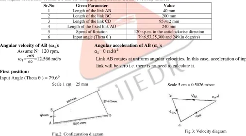
Example:ABCD is a four bar mechanism, selected for analysis purpose and its dimensions are as follows. We have to find the angular velocity and angular acceleration of links BC and CD using graphical method. (Relative velocity method)

Sr.No Given Parameter Value

1 Length of the link AB 40 mm

2 Length of the link BC 200 mm

3 Length of the link CD 95.412 mm

4 Length of the fixed link AD 240 mm

5 Speed of Rotation 120 r.p.m. in the anticlockwise direction

6 Input angle (Theta θ ) 79.6,53,25,300 and 249(in degrees)

Angular velocity of AB (𝛚𝟏): Angular acceleration of AB (𝛂𝟏): Assume N= 120 rpm, α1= 0 rad/s2

ω1=

2πN

60=12.566 rad/s Link AB rotates at uniform angular velocities. In this case, acceleration of input link will be zero i.e. there is no need to calculate it.

First position:

Input Angle (Theta θ ) = 79.60

Scale 1 cm = 25 mm

Fig.2: Configuration diagram

Angular velocity of links BC and CD

First of all, draw the configuration diagram of a four bar chain, to some suitable scale. The velocity diagram is drawn as follows: 1. Since A and D are fixed points, therefore these points lie at one place in the velocity diagram. Draw vector ab perpendicular to AB, to some suitable scale, to represent the velocity of B w.r.t. A such that

Vector ab = vBA = vB= 0.502 m/s

2. From point b, draw vector bc perpendicular to BC to represent the velocity of C w.r.t B and from point d, draw vector dc perpendicular to DC to represent the velocity of C w.r.t D. The vectors bc and dc intersect at c. By measurement, we find that

vCB = vector bc = 0.291508 m/s and vCD = vector dc = 0.462392 m/s We know that angular velocity of link BC,

ωBC=

v_CB BC =

0.291508

0.2 = 1.457 rad/s (Clockwise)

Scale 5 cm = 0.5026 m/sec

(4)

IJEDR1603129

789

and angular velocity of link CD,

ωCD=

vCD

DC =

0.462392

0.095412 = 4.8462 rad/s (Anticlockwise)

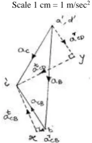
Scale 1 cm = 1 m/sec2

Fig.4: Acceleration diagram

The acceleration diagram is drawn as follows:

1. Since A and D are fixed points, therefore these points lie at one place in the acceleration diagram. Draw vector aʹbʹ parallel to AB, to some suitable scale, to represent the radial component of acceleration of B w.r.t. A such that

Vector aʹbʹ= aBAr = aB = 6.300 m/s2

2. From point bʹ, draw vector bʹx parallel to BC to represent the radial component of acceleration of C with respect to B such that Vector bʹx = aCBr = 0.4248 m/s2

3. From point x, draw vector xcʹ perpendicular to BC to represent the tangential component of acceleration of C with respect to B whose magnitude is not yet known.

4. Now from point dʹ, draw vector dʹy parallel to DC to represent the radial component of acceleration of C with respect to D Vector dʹy = aCDr = 2.2399 m/s2

5. From point y, draw vector ycʹ perpendicular to DC to represent the tangential component of acceleration of C w.r.t. D. 6. The vectors xcʹ and ycʹ intersect at cʹ. Join aʹcʹ and bʹcʹ. By measurement, we find that

atCB = vector xcʹ = 2.95 m/s2 and atCD = vector ycʹ = 3.45 m/s2 We know that angular acceleration of link BC,

αBC=

a_CBt BC =

2.95

0.2 = 14.75 rad/s

2_{(Anticlockwise)} and angular acceleration of link CD,

αCD=

a_CDt DC =

3.45

0.095412 = 36.1589 rad/s

2_{(Anticlockwise)}

Similarly we have found the the angular velocity and angular acceleration of links BC and CD for rest of the angular displacements of input link.

IV. RESULTS AND DISCUSSION:

The results are represented in tabular form given below. Input variables:

THETA = Angular displacement of the input link AB in degrees

VELA = Angular velocity of the input link AB in rad/s ACCA = Angular acceleration of the input link in rad/s2

Table 1: Results by Graphical Method

THETA (deg)

VELA

(rad/sec) ACCA PHI BETA VELC VELB ACCC ACCB

79.6 12.56 0 114 14 4.8462 -1.457 36.1589 14.75

53 12.56 0 106 17 3.0552 -2.01 61.837 15.75

Angular acceleration of links BC and CD

Since the angular acceleration of the crank AB is zero, therefore there will be no tangential component of acceleration of B with respect to A.

The radial component of acceleration of B with respect to A

arBA = aBA = aB =

v_BA2 AB =

(0.502)2

0.04 = 6.300 m/s 2

Radial component of acceleration of C with respect to B,

arCB =

v_CB2 BC =

(0.291508)2

0.2 = 0.4248 m/s 2

and radial component of acceleration of C with respect to D,

arCD = aCD = aC =

v_CD2

DC =

(0.4623)2

0.095412 = 2.2399 m/s

2

Output variables:

(5)

IJEDR1603129

790

25 12.56 0 101 22 0.210 -2.4627 80.178 8.5

300 12.56 0 125.5 34 -5.2676 0.201 -4.716 -44.75

249 12.56 0 145 28 -3.7927 2.7643 -31.442 -19.75

Table 2: Results by Analytical Method

THETA (deg)

VELA (rad/sec)

ACCA PHI BETA VELC VELB ACCC ACCB

79.6 12.56 0 -133.051 -33.046 -4.934 1.376 17.531 39.105

12.56 0 113.865 13.86 4.874 -1.436 36.176 14.602

53 12.56 0 122.125 -34.31 -5.263 -0.213 -2.136 44.684

12.56 0 105.294 17.483 3.061 -1.988 61.809 14.988

25 12.56 0 -110.97 -32.004 -4.499 -1.778 -39.503 32.334

12.56 0 101.484 22.518 0.2323 -2.488 80.532 8.693

300 12.56 0 -107.161 -16.416 3.630 -1.842 -55.196 -15.121

12.56 0 125.058 34.312 -5.251 0.221 -4.512 -44.586

249 12.56 0 -127.475 -11.062 5.791 -0.795 -5.395 -15.603

12.56 0 144.181 27.768 -3.875 2.711 -30.868 -20.660

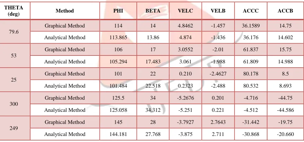
Table 3: Comparison Table of Results obtained by Graphical and Analytical Method

THETA

(deg) Method PHI BETA VELC VELB ACCC ACCB

79.6

Graphical Method 114 14 4.8462 -1.457 36.1589 14.75

Analytical Method 113.865 13.86 4.874 -1.436 36.176 14.602

53

25

300

Graphical Method 125.5 34 -5.2676 0.201 -4.716 -44.75

Analytical Method 125.058 34.312 -5.251 0.221 -4.512 -44.586

249

Graphical Method 145 28 -3.7927 2.7643 -31.442 -19.75

(6)

IJEDR1603129

791

Fig.5: Plot of Angular Displacement Fig.6: Plot of Angular Velocity

Fig.7: Plot of Angular Acceleration

A. Modelling and Simulation of Four bar links using ADAMS

ADAMS stands for Automatic Dynamic Analysis of Mechanical Systems and was originally developed by Mechanical Dynamics Inc. (MDI). ADAMS/View allows user to build, simulate and examine results in a single Graphical User Environment (GUI). It is the standard pre-processor used by MSC.ADAMS. ADAMS/Post-Processor is a combined 3D animation, plotting, and documentation tool. Full 3D view of the complete model and animation of the system dynamics is supported.

Steps of Performing a Motion Simulation

1. Create a new Adams database 2. Define units and working grid size 3. Import or create geometry

4. Define moving parts in the model

5. Connect the moving parts with joint connections Starting a New Modelling Session

When Adams/View is started, Adams/View displays a Welcome dialog box that lets one create a new modelling database or use an existing one. The GUI screen with Welcome dialog box is shown below. Double click the MSC ADAMS/View to enter ADAMS/View, the following dialogue box appears:

Step 1: Creating the model

 Click “New Model” Icon and Modify the spacing of working grid (X=300 mm, Y=200 mm)  Set the units from setting menu and Click “OK”

0 20 40 60 80 100 120 140 160

1st 2nd 3rd 4th 5th

V a lu es o f ø a n d β

Positions of Mechanism

Comparison by Graphical and Analytical Method PHI(ø) Graphical Method PHI(ø) Analytical Method BETA(β) Graphical Method BETA(β) Analytical Method -60 -40 -20 0 20 40 60 80 100

1st 2nd 3rd 4th 5th

An g u la r Ac cl no f

C D &

B C (r a d /se c 2)

Comparison by Graphical & Analytical Method

ACCC Graphical Method ACCC Analytical Method ACCB Graphical Method ACCB Analytical Method -6 -4 -2 0 2 4 6

1st 2nd 3rd 4th 5th

An g u la r v elo city o f CD & B C (r a d /se c)

Comparison by Graphical & Analytical Method VELC Graphical Method VELC Analytical Method VELB Graphical Method VELB Analytical Method

6. Apply motion to a joint 7. Run a kinematic simulation 8. Animate simulation results

(7)

IJEDR1603129

792

Fig.8: Welcome window of MSC Adams/View Fig.9: Creating the model Fig.10: Settings window

Fig.11: Creating markers of four bar mechanism

Fig.12: Defining the joints between links of the four bar mechanism Fig.13: Add the motion of the crank of the four bar mechanism

Step 5: Testing the Model

 From Simulation ribbon, select Run an Interactive Simulation  Set End Time to 2.5 and Step Size to 250

 Click start .To plot the results select the Plotting Tool from the Main toolbox. This opens up the Adams/View Post Processor Window, wherein one can select the data set needed to plot & select Add Curves to plot them & Clear Plot to clear the plot once review is completed.

 Create a CM position plots for links in different characteristics. Also create a CM angular velocity and CM angular acceleration plots for links in different characteristics.

 Use the Plot Tracking tool .Follow the Plot curve and find the angular velocity as well as angular acceleration at X=0.0 Step 2: Create a Marker

 Press F4 to open Coordinate Window

 From Bodies Ribbon, select Construction Geometry: Marker  Create a Marker at each of the following Coordinates of

designed mechanism A (0, 0, 0);

B (2.5, 40, 0); C (190,107.5, 0) and D (237.5, 27.5, 0)

Step 3: Create links and joints

 From Bodies ribbon, double click Rigid Body: Link  Create links AB, BC and CD using the markers as end

points.

 From Connectors ribbon, double click Create a Revolute joint. Make revolute joints between two links at points B and C, and between link and ground at A and D.

Step 4: Add Motion at point A

(8)

IJEDR1603129

793

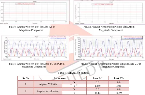
Here four bar mechanism is modelled, assembled and simulated to obtain the result at different position of links. During that different nature of graph in ADAMS on angle of link, angular velocity of link and angular acceleration verses time in anticlockwise movement of links are studied and following graphs are obtained from software.

B. Graphical representation of the simulation results:

Fig.14: Position Plots for Links AB, BC and CD in XComponent Fig.15: Position Plots for Links AB, BC and CD in Y Component

Fig.16: Angular velocity Plot for Link AB in Fig.17: Angular Acceleration Plot for Link AB in

Magnitude Component Magnitude Component

Fig.18: Angular velocity Plot for Links BC and CD in Fig.19: Angular Acceleration Plot for Links BC and CD in

Magnitude Component Magnitude Component

Table 4: ADAMS Solution

Sr.No Parameters Link BC Link CD

1 Angular Velocity X 0.0 0.0

Y 1.449 5.06

2 Angular Acceleration X 0.0 0.0

Y 14.14 36.99

From the above table it is clear that the values obtained by simulation with ADAMS software are near about same with results obtained by analytical and graphical method for first position of mechanism. We can get the results for any position of mechanism.

V. CONCLUSION:

The analytical method using computer programming is useful and easier in determining the values of velocity and acceleration analysis at different positions of the crank as compared to graphical method. Modelling and simulation using simulating software ADAMS is very fast, less laborious and very efficient than graphical, analytical method. Adams Multibody dynamics software enables engineers to easily create and test virtual prototypes of mechanical systems in a fraction of the time. Results obtained using ADAMS is found to be in agreement with the results obtained from graphical and analytical method. Results are obtained in form of time diagram of the desired variables. MSC Adams/View was used as a tool which allows a better simulation and visualization of the model and easier evaluation of the results obtained.

(9)

IJEDR1603129

794

[1] G. Kamat, G. Hoshing, A. Pawar, A. Lokhande. P. Patunkar and S. Hatawalane, “Synthesis and Analysis of Adjustable

Planar Four-bar Mechanism”, International Journal of Advanced Mechanical Engineering, vol.4, issue 3, pp.263-268, 2014.

[2] Dr R. P. Sharma, ChikeshRanjan, “Modelling And Simulation of Four-Bar Planar Mechanisms Using Adams”, International Journal of Mechanical Engineering and Technology (IJMET), ISSN 0976 – 6340(Print), ISSN 0976 – 6359(Online) Volume 4, Issue 2, March - April (2013)

[3] A. K. Kapse, Dr. C. C. Handa, “A Generalized Approach for Measurement of Performance of Planar Mechanism Using Relative Velocity Method”, International Journal of Engineering Research and Applications(IJERA), ISSN: 2248-9622, Vol. 2, Issue4, pp.1871-1573, July-August 2012

[4] Mulla Abdulkadar, Bhagyesh Deshmukh, “Simulation of Four Bar Mechanism for Path Generation”, International Journal of Emerging Technology and Advanced Engineering, ISSN 2250-2459, ISO 9001:2008 Certified Journal, Volume 3, Issue 9, September 2013

[5] Prof. N. G. Alvi, Dr. S. V. Deshmukh, Ram. R. Wayzode, “Computer Aided Analysis of Four bar Chain Mechanism”, International Journal of Engineering Research and Applications (IJERA), ISSN: 2248-9622, Vol. 2, Issue 3, pp. 286-290, May-Jun 2012

[6] DarinaHroncova, Michal Binda, PatrikSarga, Frantisek Kick, “Kinematical analysis of crank slider mechanism using MSC Adams/View”, SciVerseScience Direct Procedia Engineering ,48 ( 2012 ) 213 – 222

[7] R. S. Khurmi & J. K Gupta, “Theory of Machines”, S. Chand Publication, 2010 [8] S. S. Rattan, “Theory of Machines”, Tata McGraw-Hill Publication, 2008