Optimization of a boundary element approach to electromagnet design with application to a host of current problems in Magnetic Resonance Imaging

(1)

Electronic Thesis and Dissertation Repository

8-16-2013 12:00 AM

Optimization of a boundary element approach to electromagnet

design with application to a host of current problems in Magnetic

Resonance Imaging

Chad T. Harris

The University of Western Ontario

Supervisor

Dr. Blaine Chronik

The University of Western Ontario Graduate Program in Physics

A thesis submitted in partial fulfillment of the requirements for the degree in Doctor of Philosophy

Follow this and additional works at: https://ir.lib.uwo.ca/etd

Part of the Electrical and Computer Engineering Commons, Physics Commons, and the Radiology Commons

Recommended Citation Recommended Citation

Harris, Chad T., "Optimization of a boundary element approach to electromagnet design with application to a host of current problems in Magnetic Resonance Imaging" (2013). Electronic Thesis and Dissertation Repository. 1422.

https://ir.lib.uwo.ca/etd/1422

This Dissertation/Thesis is brought to you for free and open access by Scholarship@Western. It has been accepted for inclusion in Electronic Thesis and Dissertation Repository by an authorized administrator of

(2)

MAGNETIC RESONANCE IMAGING

(Thesis format: Integrated Article)

by

Chad Tyler Harris

Graduate Program in Physics

A thesis submitted in partial fulfillment of the requirements for the degree of

Doctor of Philosophy

The School of Graduate and Postdoctoral Studies The University of Western Ontario

London, Ontario, Canada

(3)

ii

Magnetic resonance imaging (MRI) has proven to be a valuable methodological approach in both basic research and clinical practice. However, significant hardware advances are still needed in order to further improve and extend the applications of the technique. The present dissertation predominantly addresses gradient and shim coil design (sub-systems of the MR system).

A design study to investigate gradient performance over a set of surface geometries ranging in curvature from planar to a full cylinder using the boundary element (BE) method is presented. The results of this study serve as a guide for future planar and pseudo-planar gradient systems for a range of applications.

Additions to the BE method of coil design are developed, including the direct control of the magnetic field uniformity produced by the final electromagnet and the minimum separation between adjacent wires in the final design.

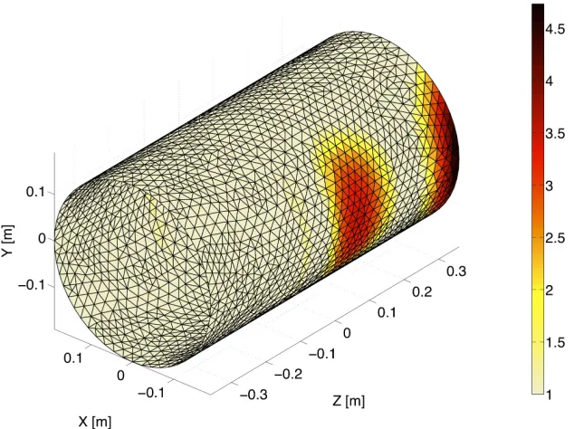
A method to simulate induced eddy currents on thin conducting surfaces is presented. The method is used to predict the time-dependent decay of eddy currents induced on a cylindrical copper bore within a 7 T MR system and the induced heating on small conducting structures; both predictions are compared against experiment. Next, the method is extended to predict localized power deposition and the spatial distribution of force due to the Lorentz interaction of the eddy current distribution with the main magnetic field.

New methods for the design of actively shielded electromagnets are presented and compared with existing techniques for the case of a whole-body transverse gradient coil. The methods are judged using a variety of shielding performance parameters.

A novel approach to eliminate the interactions between the MR gradient system and external, non-MR specific, active devices is presented and its feasibility is discussed.

(4)

iii

Keywords

(5)

iv

Co-Authorship Statement

This thesis contains materials from the following manuscripts:

C.T. Harris, W.B. Handler, B.A. Chronik. “Design study to investigate the effect of curvature on gradient coil performance for localized regions of interest”. Concepts in Magnetic

Resonance Part B: Magnetic Resonance Engineering, 41B(2):62-71 (2012). [DOI: 10.1002/cmr.b.21212]

C.T. Harris, W.B. Handler, B.A. Chronik. “Electromagnet design allowing explicit and simultaneous control of minimum wire spacing and field uniformity”. Concepts in Magnetic Resonance Part B: Magnetic Resonance Engineering, 41B(4):120-129 (2012). [DOI:

10.1002/cmr.b.21220]

C.T. Harris, D.W. Haw, W.B. Handler, B.A. Chronik. “Application and experimental validation of an integral method for simulation of gradient-induced eddy currents on

conducting surfaces during magnetic resonance imaging”. Physics in Medicine and Biology, 58(12):4367-4379 (2013).

C.T. Harris, D.W. Haw, W.B. Handler, B.A. Chronik. “Shielded electromagnets of arbitrary surface geometry using the boundary element method and a minimum energy constraint”. Journal of Magnetic Resonance, (accepted June 18, 2013). Submission #: JMR-12-316R2.

C.T. Harris, W.B. Handler, B.A. Chronik. “A new approach to shimming: The dynamically controlled adaptive current network”. Magnetic Resonance in Medicine, Article first

published online (March 15, 2013). [DOI: 10.1002/mrm.24724]

(6)

v

(7)

vi

Dedication

To my family,

(8)

vii

Acknowledgments

There are so many people to acknowledge with respect to this work.

First off I would like to thank my supervisor Dr. Blaine Chronik. His guidance throughout my PhD work has been instrumental to my growth as a researcher and a person. I cannot imagine a better mentor to look up to.

Next, I would like to thank Dr. Will Handler. Without him most of this work would still be ideas in my head. He has acted as a second supervisor to me. I’m going to greatly miss our discussions over coffee on topics ranging from new science to politics.

The extensive knowledge and expertise that Brian Dalrymple and Frank Van Sas have provided of construction methods has helped immensely to keep my ideas grounded in reality.

Dr. Tim Scholl has been very helpful and supportive throughout my tenure at Western, acting in a supervisory role, as a collaborator, and as a friend.

I’ve had the pleasure and privilege to work with many talented researchers throughout my tenure in the MRI systems development lab – Kyle Gilbert, Rebecca Feldman, James

Odegaard, Josh de Bever, Jamu Alford, Dustin Haw, Parisa Hudson, and Geron Bindseil – as well as some very able undergraduate students – James Hopkins, Andrew Boivin, Leesa Fleury, and Christopher Brown.

I would like to thank Doug Hie for his guidance and conversations on the choice of switch component for the adaptive shim project.

I am grateful to Joe Gati, Kim Krueger, Adam McLean, and Oksana Opalevych for training me to operate the 3 T MRI scanner at the Robarts Reseach Institute; the experience has been invaluable to my research development.

(9)

viii

List of Tables

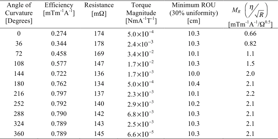
Table 2-1. Performance properties of the x-gradient coil as a function of the angle of

curvature.a ... 38!

Table 2-2. Performance properties of the y-gradient coil as a function of the angle of

curvature. a_{... 39}_!

Table 2-3. Performance properties of the z-gradient coil as a function of the angle of

curvature.a ... 39!

Table 2-4. Intrinsic and performance properties of the x-, y-, and z-gradient coils for 180° of curvature.a_{... 41}_!

Table 3-1. Intrinsic and performance properties for the three transverse head and neck

gradient coils designed with 16 iterations of the algorithm. ... 59!

Table 3-2. Intrinsic and performance properties for the B0-offset polarizing coil designed

with 15 iterations of the algorithm over two coaxial cylindrical mesh layers. ... 61!

Table 4-1. Reduced chi-square values for the fit between the simulation and experimental data. ... 80!

Table 4-2. Simulated and experimentally measured heating rates for a 5 cm x 5 cm copper square at two different thicknesses for multiple frequencies. ... 83!

Table 5-1. Design parameters and performance properties for minimum inductance coils designed using shielding methods 1 – 5. ... 126!

Table 5-2. Design parameters and performance properties for minimum power coils designed using shielding methods 1 – 5. ... 127!

Table 5-3. Comparison of performance properties between the coil designed using the BE method in this work and the coil design reported by Shvartsman et al. (2005). ... 143!

(17)

xvi

Table 6-3. Performance properties of rectangular, z-gradient shield. ... 155!

Table 7-1. Performance properties of the simulated adaptive shim coil wire patterns for ROI #1 and #2. ... 175!

Table A-1. Total computation time for each version of code for the transverse gradient coil example. ... 228!

(18)

xvii

List of Figures

Figure 1.1. Sagittal (a) and axial (b) slice images of a human brain. This image was taken

with a 3 T Siemens Tim Trio system at the Robarts Research Institute in London, Canada. ... 1!

Figure 1.2. (a) A “body” radiofrequency (RF) coil that has been removed from the bore of a 3 T MR scanner. This coil is capable of receiving RF magnetic fields; however it is typically only used for transmission. (b) A local 32 channel “head-only” RF receive coil. This coil is designed to conform closely to the head to maximize signal detection. Due to its high receive sensitivity; it is used at the Robarts Research Institute in London, Ontario, Canada for fMRI studies in the human brain. ... 8!

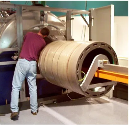
Figure 1.3. A whole-body gradient set after removal from a superconducting MR system. The gradients are immersed in epoxy to prevent the wires from shifting due to Lorentz forces while being pulsed for imaging. ... 11!

Figure 1.4. (a) Stream function for an x-gradient coil design over a cylindrical surface. (b)

Wire pattern of the x-gradient coil obtained by contouring the stream function in (a) with 10

contours. In (b), red and blue denote positive and negative current flow with respect to the x

-axis. ... 22!

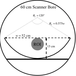
Figure 2.1. Schematic of placement of curved-planar gradient coil within 60 cm scanner bore.

The geometry shown has radius of curvature, Rc, equal to approximately 0.575 times the total

width of the coil, w = 2x. Note: w is constrained to 0.52 m. This value of Rc corresponds to an

angle of curvature equal to θc= 120° via equation (2.1). ... 34!

Figure 2.2. X-(a, d, g, j, m), Y-(b, e, h, k, n), and Z-(c, f, I, l, o) gradient coil patterns for five

different angles of curvature: (a-c) planar (0°), (d-f) 108° curvature, (g-i) half-cylindrical

(180°), (j-l) 288° curvature, and (m-o) full-cylindrical (360°). ... 36!

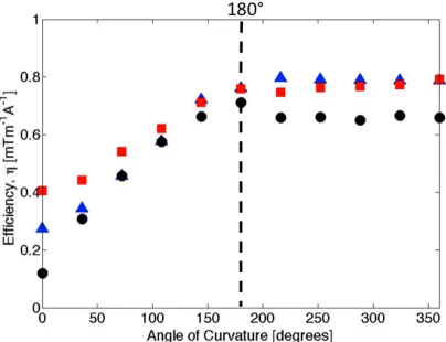
Figure 2.3. Gradient efficiency scaled for 800 µH inductance versus angle of curvature for

(19)

xviii

for the x- (a-c), y- (d-f), and z- (g-i) gradient coils for 180° curvature. Contours are shown for 10%, 30%, and 50% gradient uniformity. The region of interest, constrained to have at least 30% uniformity, is shown in all three planes and the coil surface is shown as a thick line in the xy-plane. ... 40!

Figure 3.1. Outward pointing normal vectors for triangular element j with node indices 1, 2, and 3. ... 49!

Figure 3.2. Flow chart of calculations for the combined algorithm to find the optimal relative weighting between localized power dissipation and field uniformity. ... 52!

Figure 3.3. Finite element mesh geometry of the transverse head coil cylindrical surface and target field positions for: (a) the large ROU composed of 2452 target points distributed over a spherical region 24 cm in diameter and (b) the small ROU composed of 2452 target points distributed over a spherical region 10 cm in diameter. Both ROUs were centered 12 cm inward from the edge of the cylindrical surface at the point (x, y, z)center = (0, 0, -0.24) m. ... 54!

Figure 3.4. (a) Minimum wire separation vs. number of iterations of algorithm; (b) Maximum gradient uniformity over three 24 cm diameter circles (one in each plane) centered about the imaging region vs. iteration number. ... 56!

(20)

xix

Figure 3.6. Wire pattern of the uniform field coil for the (a) inner-layer, at a diameter of 30 cm; and (b) outer-layer, at a diameter of 30.5 cm. Both layers were constrained to a

maximum length of 30 cm in the z-direction. Arrows denote relative current direction. ... 60!

Figure 3.7. Field homogeneity plots for the (a) xy- and (b) yz-planes of the uniform field coil depicted in Figure 6. The 1% field uniformity region extends roughly 10 cm radially and 15 cm in the z-direction. ... 60!

Figure 3.8. Visualization of the relative localized power weighting. The colour bar corresponds to the relative β value for each triangular element. Note how the power

weighting is largest near the far edge of the coil; therefore, increasing the length of the coil geometry would most likely increase performance. ... 63!

Figure 4.1. (a) – (d) Display the first four eigenmodes of the U matrix for a cylindrical

surface respectively. ... 71!

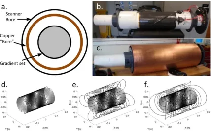
Figure 4.2. (a) Schematic of the gradient coil within the artificial copper bore, all within the scanner bore. (b) Constructed gradient set with adjustable shield. (c) Gradient set placed within copper bore. (d-f) Primary and shield orientations simulated: d) unshielded primary coil; e) shielded primary coil with shield rotated 45°; f) shielded primary coil with shield aligned. ... 74!

Figure 4.3. a) Copper square used for heating experiment (dimensions: 5 cm x 5 cm x 0.53 mm). (b & c) Placement of the eight thermocouples used to measure the temperature increase of the copper square during the experiment (lines drawn on the copper correspond to 1 cm intervals). (d) Power solenoid used for the inductive heating experiment. (e) Computer model representation of the power solenoid shown in d) and the copper square represented as a finite element mesh. ... 78!

(21)

xx

copper square (thickness = 0.53 mm) and (b) thick copper square (thickness = 3.10 mm). The dotted lines on either side of the simulation values represent upper and lower bounds due to errors in constants used in the simulation (such as the resistivity of copper). Error bars on the experimental values are smaller than the data points shown. ... 82!

Figure 4.6. Simulated temperature rise for the thin copper square versus frequency calculated using the time-domain solver (red triangle) and the frequency-domain solver (blue circle). The maximum percent difference between their solutions over this range of frequencies was less than 2%. ... 87!

Figure 4.7. (a) Wire pattern of the primary z-gradient coil (gray) with active shield (black),

within a copper cylinder (brown). (b) Current waveform consisting of a trapezoid pulse with a rise time of 800 µs and flattop duration of 40 ms. ... 91!

Figure 4.8. (a) Time-domain and frequency-domain solutions of the induced magnetic field

in µT at the position (x, y, z) = (0, 0, 5 cm). (b) Absolute value of the percent difference of

the two solutions over the first ramp and decay. The plot is shown up until 4.5 µs at which point the magnitude of the induced field was less than 0.5 µT. ... 92!

Figure 4.9. Spatial density of energy deposited into the conducting square as a function of position over one sinusoidal cycle of dB/dt = 39 T/s at a frequency of 1 kHz. ... 95!

Figure 4.10. Finite element mesh of the conducting square. The inner (red triangles) and outer (blue circles) elements used for heating rate comparisons are shown. ... 97!

Figure 4.11. Heating rate of the inner and outer elements (Fig. 4.10) as a function of time. Shown with the average heating rate of the square, calculated in section 4.1. ... 98!

Figure 4.12. Finite element mesh model of the half pacemaker casing. The material of the

casing was specified to be titanium with a resistivity of 6 x 10-7 Ωm. The thickness of the

(22)

xxi

Figure 4.13. Typical orientation of a pacemaker casing (shown in red) on the human body within an MR scanner if an image of the torso was being performed. ... 100!

Figure 4.14. Orientation of the pacemaker casing with respect to the y-gradient coil that was used in simulation. The pacemaker casing was offset 15 cm, 5 cm, and 20 cm in the x-, y-, and z-directions respectively. Note that only the pacemaker mesh geometry, the gradient coil wire pattern, and the pulse sequence are used in the simulation. ... 101!

Figure 4.15. Distribution of deposited energy over the pacemaker casing for one sinusoidal cycle of the y-gradient coil driven at 5 kHz at 80 mT/m. ... 102!

Figure 4.16. Pressure in kPa normal to the pacemaker casing surface 8.16 µs into the

sinusoidal cycle. ... 105!

Figure 4.17. Pressure in kPa normal to the pacemaker surface for a single element over the entire sinusoidal cycle. ... 106!

Figure 5.1. (a) Primary and shield mesh surfaces shown with the spherical set of target field points used for optimization. (b) Primary and shield surfaces with the same spherical set of target points in the ROI and additional shielding points for shielding method described in 5.1.1. (c) Primary and shield surfaces shown within the external cryostat surface extending 1.5 m in the z-direction with a diameter of 1 m. ... 120!

Figure 5.2. Comparison of performance parameters for the minimum power shielded gradient coil designs. (a) Fringe field merit MFF, (b) deposited power in the cryostat merit value

MRcryo, (c) induced field merit MBEC, and (d) induced gradient merit MGEC. ... 128!

Figure 5.3. Comparison of performance parameters for the minimum inductance shielded gradient coil designs. (a) Fringe field merit MFF, (b) deposited power in the cryostat merit value MRcryo, (c) induced field merit MBEC, and (d) induced gradient merit MGEC. ... 129!

Figure 5.4. Dimensions of the vertical field, open-geometry, permanent magnet MR system. The rectangular bore has dimensions of 85 cm in width and 46 cm in height. ... 134!

(23)

xxii

the insert geometry. The primary mesh consists of 1077 nodes and 2058 elements, the shield mesh consists of 2012 nodes and 3844 elements. ... 135!

Figure 5.6. Wire pattern for the cylindrical primary and rectangular shield electromagnets. The wire patterns have been scaled down for ease in visualization. In this figure, colour denotes the relative direction of current flow with respect to the y-axis. ... 136!

Figure 5.7. (a) One side of the bi-planar surface over which the x-gradient coil was designed. The inner diameter of the surface is 1.1 m. (b) Finite element mesh representation of the bi-planar surface. This mesh contained 17140 nodes and 22152 triangular elements. (c) Side-view of the bi-planar surface. The diameter of the outer surface is 1.2 m; the distance

between outer and inner surfaces is 3 cm; the distance between sides of the surface is 40 cm. The target points used for optimization are also shown in blue. The target points were distributed over the surface of an ellipse of 40 cm diameter in the xy-plane and 30 cm in the

z-direction. ... 138!

Figure 5.8. Wire pattern for the bi-planar, self-shielded, x-gradient coil. Colour denotes current direction with respect to the y-axis. ... 139!

Figure 5.9. Gradient field uniformity for the x-gradient coil shown in Figure 5.8 over the xy- (a), zx- (b), and yz-planes (c). Contour lines are shown for (5 %, 10 %, 15 %, 20 %, 25 %, and 30 %). (d) Base 10 logarithm of the magnitude of the magnetic field for one-quadrant of the zx-plane spanning 60 cm in the z-direction and 1 m in the x-direction. The shielding wires on the outer surface of the coil act to reduce the magnetic field outside of the imaging region. ... 140!

(24)

xxiii

Figure 6.1. (a) Finite element mesh of the spherical shield geometry. (b) Position of spherical geometry within the bore of a whole-body transverse gradient coil. (c) Position and

distribution of target points within the spherical shield geometry. ... 149!

Figure 6.2. Finite element mesh of the rectangular shield with backside removed. The target points used for current density optimization are shown within the mesh, distributed

throughout an elliptical region. ... 151!

Figure 6.3. (a) Wire pattern for the transverse shield coil. (b) Gradient uniformity over the xy -plane when the spherical shield shown in (a) is present. (c) Magnitude of the magnetic field along the z-axis on a line through the center of the shield (x, y) = (12.5, 12.5) cm. ... 153!

Figure 6.4. (a) Wire pattern for the longitudinal shield coil. (b) Gradient uniformity over the

xy-plane when the spherical shield shown in (a) is present. (c) Magnitude of the magnetic field along the z-axis on a line through the center of the shield (x, y) = (12.5, 12.5) cm. ... 154!

Figure 6.5. (a) Wire pattern for the practical, rectangular, longitudinal shield coil. (b)

Gradient uniformity over the zx-plane when the shield shown in (a) is present. Note how the presence of the shield has very little effect on the region of gradient uniformity. ... 156!

Figure 7.1. Visualization of two separate current pathways depending on which MOSFETs are in the open or closed state. ... 164!

Figure 7.2. Schematic depiction of the adaptive shim MOSFET network used for the computer simulations. The mesh network is shown with a human head inserted into the cylindrical former. In reality an RF coil would be placed within the cylindrical shim as well. Note that both surfaces of the cylindrical former contain a network; one surface would produce the wire pattern while the other surface would provide pathways between ‘thumbs’ for complicated wire patterns. ... 166!

(25)

xxiv

and (c) ROI #2. Realistic wire patterns (black) produced by superimposing the smooth pattern (gray) onto a finite mesh network of discretization dimension of 1 cm x 1 cm for (b) ROI #1 and (d) ROI #2. Note the small loop and sharp corners of the smooth pattern in (b) are not matched exactly in the realistic meshed pattern. ... 169!

Figure 7.5. (a) Cylindrical mesh network of ¼” copper tape. (b) Final constructed proof-of-principle coil with 14 MOSFETs positioned to allow two distinct current pathways. (c) Proof-of-principle coil shown within Siemens Head/Neck RF matrix and ready for insertion into MR scanner. (d) Current path for the “gradient” field profile. (e) Current path for the “constant” field profile. Note the changes in current direction between (d) and (e). ... 171!

Figure 7.6. Field maps for ROI # 1 (a-c) and ROI # 2 (d-f) for: (a, d) no additional shim coil; (b, e) simulated smooth shim coil wire pattern present; (c, f) simulated discretized shim coil wire pattern present. ... 173!

Figure 7.7. Histogram plots of the magnetic field inhomogeneity over ROI # 1 (a) and ROI # 2 (b). For each set of histograms, the plot on the left is with no additional shim coil, the middle plot is with the simulated smooth shim wire pattern present and the plot on the right is with the simulated discretized shim wire pattern present. Each histogram was fit with either a Gumbel or Gaussian distribution (depending on the degree of skew) and FWHM values were extracted. ... 174!

Figure 7.8. Predicted (a, c) and measured (b, d) magnetic field profiles of the

proof-of-principle coil for the (a, b) “gradient” field mode and (c, d) “constant” field mode. ... 176!

Figure A.1. Two streamlines ψ(P1) and ψ(P2). The total flux passing through a curve

χ between P1 and P2 is equal no matter the shape of the curve. ... 197!

Figure A.2. (a) Example stream function shown with five contour lines (black lines) to approximate the current density. (b) The magnitude of the corresponding current density from the stream function shown in (a). The contour lines from (a) are projected down into the

xy-plane. Note how the current density is largest where the stream function contains a

(26)

xxv

Figure A.3. (a) Continuous, smooth, curved surface geometry. (b) Finite element mesh

representation of the surface in (a). ... 199!

Figure A.4. Finite element mesh surface from Figure A.3. Along the lower edge of the surface boundary nodes are highlighted in red. In the zoomed in section (inset right), triangular element m is shown with nodes i, j, and k as vertices. Also shown on the finite mesh surface is the outward pointing normal vector, n (upper left hand side). ... 201!

Figure A.5. The linear shape functions over a triangular element: (a) N1 from equation

(A.20), (b) N2 from equation (A.21), and (c) N3 from equation (A.22). ... 204!

Figure A.6. The current basis set for triangular elements 1 – 6 encircling node n. They are equal to the vector of the edge opposite the node divided by twice the elemental area. ... 206!

Figure A.7. Visualization of condensing an N x N matrix to an N’ x N’ matrix with two edges. ... 214!

Figure A.8. (a) Stream function for an x-gradient coil design over a cylindrical surface. (b) Wire pattern of the x-gradient coil obtained by contouring the stream function in (a) with 10 contours. In (b), red and blue denote positive and negative current flow with respect to the x -axis. ... 217!

Figure A.9. Normalized performance parameters versus the number of triangular elements within a cylindrical mesh. The cylindrical surface used was 1 m in diameter and 2 m long; the region of interest was a sphere 40 cm in diameter. The performance parameters found were the maximum gradient uniformity over the surface of the region of interest and the resistive and inductive merit values. Prior to plotting the parameters were normalized using their values calculated at the smallest mesh discretization (9376 elements). ... 218!

Figure A.10. The three different mesh sizes used for the analysis of code optimization. The same cylindrical surface can contain either (a) 310 nodes and 588 elements (“Fine”), (b) 1398 nodes and 2732 elements (“Extra Fine”), or (c) 4282 nodes and 8460 elements

(27)

xxvi

toolbox for (a) CV1 and (b) CV2. In this example the design problem contained 4282 nodes in the mesh surface and 400 target points. Note how the calculation times for the calculation of the node basis functions and the resistance matrix (columns 1 and 2 in the graphs

respectively) have decreased dramatically after optimization. ... 222!

Figure A.12. Computation times for the five most time-dominant functions in the design toolbox for (a) CV2 and (b) CV3. In this example the design problem contained 4282 nodes in the mesh surface and 400 target points. The calculation of the field matrix decreases dramatically from a few minutes to less than 10 seconds using CV3. ... 223!

Figure A.13. Computation times for the five most time-dominant functions in the design toolbox for (a) CV3 and (b) CV4. In this example the design problem contained 4282 nodes in the mesh surface and 400 target points. The calculation time of the 3D contouring

algorithm decreases significantly while the computation time for the field matrix calculation does not. ... 225!

Figure A.14. Comparison of the field matrix calculation times between CV3 and CV4 for design problems containing a 4282 node mesh and 400 and 8000 target points. The

difference in computation time is not significant for a small number of field targets (400 in this case); however, for 8000 target points the calculation time is reduced from just over 3 minutes to approximately 16 seconds. ... 226!

Figure A.15. Logarithm of calculation time for each version of Boundary Element method code. Times shown for 8000 target points and an ‘Extremely Fine’ mesh (blue circle); ‘Extra Fine’ mesh (red triangle); and ‘Fine’ mesh (green square). ... 227!

(28)

xxvii

(29)

xxviii

Preface

This thesis work initially started as a means of extending the necessary hardware required for delta relaxation enhanced magnetic resonance (dreMR) imaging to humans. A detailed description of the dreMR method will not be included here; instead I refer the interested reader to the journal article:

Alford J.K., Rutt B.K., Scholl T.J., Handler W.B., Chronik B.A. Delta relaxation enhanced MR: Improving activation-specificity of molecular probes through R1 dispersion imaging.

Magn Reson Med, 61(4), 796-802.

In the dreMR method, an auxiliary field-shifting insert coil is needed to temporally modify the main magnetic field in an otherwise normal superconducting 1.5 T MR system. The field-shifting insert coil must be capable of field-shifts on the order of hundreds of millitesla (mT) without negatively interacting with the main superconducting magnet. DreMR insert systems designed for small-animal imaging have been able to achieve these two necessary properties relatively easily; the small bore required for murine imaging allows the use of an actively shielded solenoidal design. This is not the case for a dreMR system intended for human imaging. Specifically, the already restricted bore width of MR systems paired with the necessity for a powerful primary electromagnet and active shield require that a field-shifting insert system for human imaging be designed on an open geometry (i.e. non-cylindrical). This inevitability was the main drive for the development of much of the subsequent work presented in this thesis (certainly Chapters 2 & 3).

(30)

xxix

devices, which itself was a consequence of the creation of the induced eddy current computational modeling tool described in Chapter 4.

Chapter 7 describes a new approach to shimming utilizing a dynamically controlled adaptive current network, which is the only work in this assembly that was not directly influenced by the desire for human dreMR imaging hardware. Instead, it stemmed from a combination of previous work done by Parisa Hudson et al. on local custom shim design (Hudson et al., Proc ISMRM 18, 2010, p.221) and techniques developed in Chapter 3 of this work to control the minimum wire separation of electromagnets during optimization.

After the aforementioned description of the motivation behind the content within this work it is ironic that the development of hardware for human dreMR imaging is not included in this thesis. This is not to stay that significant advancements in this topic have not been achieved during my Ph.D. candidacy. Indeed, I have authored and co-authored multiple works that have been presented at scientific conferences (9 in total). Of particular significance is the development of three practical designs for human dreMR insert systems: one for the human head (Harris et al., Proc ISMRM 19, 2011, p.1839); one for the torso (Harris et al., Proc ISMRM 20, 2012, p.2576); and one for the breast (Harris et al., Proc ImNO 10, 2012, p.82). Furthermore, the advanced shielding techniques presented in Chapter 5 have led to improved design and construction methods for small-animal dreMR systems (Harris et al.,

Development and Optimization of Hardware for Delta Relaxation Enhanced Magnetic Resonance Imaging. Magn Reson Med, (submitted May 29, 2013. MRM-13-14272)). The main reason for the exclusion of these works is simply to prevent this thesis from being excessively long and tedious.

I am extremely proud of each and every one of the chapters presented in this work and I hope they are well received by the reader.

(31)

Chapter 1

1 Introduction to Magnetic Resonance Imaging (MRI)

Over the past 75 years, beginning in 1938, nuclear magnetic resonance (NMR) has arisen from strictly laboratory experiments (Rabi et al., 1938, Bloch, 1946, Purcell, Torrey, & Pound, 1946) to one of the most important medical technologies of the current day. In Canada specifically, the number of MRI systems has more than doubled from 149 in 2003 to 308 in 2012 (CIHI, 2013).

One of the reasons MRI has become so important for medical diagnosis is the incredible soft tissue contrast that it provides. Figure 1.1 (a) and (b) display sagittal and axial cross-section views of a human brain respectively; one can see fine details of the brain and easily distinguish the boundary between white and gray matter in the cerebrum. Nearly all MRI scans image the distribution of hydrogen nuclei in the body; by altering the method and timing parameters of how the image is acquired, one can obtain different contrast between tissue types.

Figure 1.1. Sagittal (a) and axial (b) slice images of a human brain. This image was taken with a 3 T Siemens Tim Trio system at the Robarts Research Institute in London, Canada.

(32)

chapter is rather to introduce the reader to the concepts necessary for understanding the subsequent methods and techniques presented later in the text. The chapter will begin with a very brief description of how an MR signal and image can be created and acquired from a classical perspective. Next, the main hardware components of the system

necessary to obtain an image are described, including novel MR “insert” gradient systems. Next, a short description of magnetically induced “eddy-currents”, a common problem in MRI, is provided. Lastly, a full review of gradient and shim coil design methodologies is given with an introduction to the boundary element method of coil design. This last section is extremely important in understanding the advancements that this work provides over previous efforts.

1.1 Obtaining an NMR signal and image

All atoms that have a non-zero nuclear spin angular momentum can produce an NMR signal (Nishimura, 1996, Chapter 3). Atoms obtain this property by containing either an odd number of protons and/or an odd number of neutrons. In a classical view, atoms with nuclear spin can be thought of as spinning charged particles and hence posses a magnetic moment (Cowan, 1997, Chapter 1). In the clinical setting, the nuclear spin of interest is hydrogen. This is largely due to the relatively high abundance of hydrogen in biological tissue and the high value of its magnetic moment. From this point onward, whenever nuclear spins or magnetic moments are mentioned they explicitly refer to hydrogen protons, which have a spin equal to 1/2.

In the absence of any external magnetic field, the magnetic moments within a tissue sample are randomly oriented and therefore their net magnetization is zero. However, in the presence of an external magnetic field the individual magnetic moments have a slight tendency to align with the field. This affinity, which will create a net magnetization

M(r,t), is only detectable when dealing with large quantities of magnetic moments due to

the relatively high thermal energy of protons in biological tissue. Luckily, there is a large abundance of hydrogen in tissue, on the order of Avagadro’s number. When in thermal

(33)

proton density, ρ, the gyromagnetic ratio, γ, the external magnetic field, B0, and inversely

proportional to temperature, T

M0=

ργ2_2_B 0

4kT (1.1)

where ħ is Planck’s constant divided by 2π and k is Boltzmann’s constant. It is this

magnetization that is the source of the signal of an MR image.

In addition to the creation of magnetization throughout tissue by the application of an external magnetic field, the nuclear spins will precess at a well-defined frequency, known as the Larmor frequency. This frequency is given by the relation:

f = γ

2π B0 (1.2)

where B0 is the magnitude of the applied magnetic field, B0, along the direction of

precession, typically oriented along the z-axis, and γ, the constant known as the

gyromagnetic ratio, is specific to the particular nuclear spin of interest. For hydrogen, γ

/2π equals 42.577 MHz/T. Hence, in MRI, where typical applied magnetic fields are in

the range of 1.0 T – 3.0 T, the frequency of precession of hydrogen protons is in the radiofrequency (RF) range.

In order to obtain a signal, the magnetization is excited out of equilibrium by the

application of a magnetic pulse of RF radiation tuned to the Larmor frequency. The pulse is applied perpendicular to the static polarizing field and hence will produce a torque on the net magnetization, due to the angular analogue of Newton's second law, rotating it into a plane perpendicular to the polarizing field. After excitation, the net magnetization will continue to precess in this plane, which will induce an EMF in a nearby receiver coil (positioned to be sensitive only to magnetization in this plane) due to Faraday’s law of induction. This is the signal that is obtained during an MR experiment.

(34)

contained in the signal and an image could not be formed. This is of little use for medical imaging. In order to imbed spatial information into the signal, additional magnetic fields are applied that vary linearly with respect to the three Cartesian axes. These fields are called gradient fields and are created by additional electromagnets called gradient coils (section 1.2.3.1). The gradient coils are powered on and off during an MR pulse sequence in order to encode spatial information into the frequency and phase of the net

magnetization. One can then convert the spatially dependent frequency and phase data into an image by use of Fourier techniques (Nishimura, 1996, Chapters 2 & 3).

1.1.1 Field inhomogeneities

The method of spatial encoding of the NMR signal described above is highly dependent on the notion that the only deviation in frequency of the signal from the resonant

frequency (equation (1.2)) is due to the applied gradient field, which the user specifies.

This fails to be true when the main magnetic field, B0, contains imperfections. For

instance, if the main magnetic field contains spatial variations given by the expression:

B₀real₍_r₎

=B₀+ΔB(r) (1.3)

where B₀real(r) is the “real” main magnetic field profile and ΔB(r) are the local magnetic

field inhomogeneities, then the phase accrual of the signal after a linear x-gradient, G, is

applied for a certain time t will be:

φtotal(r)=γ x G 0 t

∫

dτ+ ΔB(r)

0

t

∫

dτ

#

$

% &

'

(=φgradient(x)+φΔB(r). (1.4)

The total phase of the signal is now the phase due to the applied gradient as well as a locally varying offset due to the local field inhomogeneity. This will obviously pose a problem if the local phase offset is comparable in value to the phase due to the gradient.

(35)

System imperfections are simply the result of the main magnetic field not being

completely uniform after construction. These imperfections are typically static in nature and are dealt with to a large degree at the time of system installation. Field

inhomogeneities after system installations are normally in the range of 10 parts per million (ppm) peak-to-peak over a 50 cm diameter volume (Cosmus & Parizh, 2011).

Sample induced field inhomogeneities are caused by differences in magnetic

susceptibility between two materials at their interfaces, such as tissue-tissue interfaces or air-tissue interfaces. Inhomogeneities of this nature are typically a few ppm (Truong et al., 2002) and must be dealt with on a sample-by-sample basis. Active shim coils (section 1.2.3.3) are used to reduce these field imperfections.

The topic of time-varying magnetic fields and their subsequently induced eddy currents are discussed in detail in section 1.3 and Chapter 4 of this work. At this point in this discussion one only need know that during MR imaging eddy currents can be induced on conducting structures within the system and result in parasitic magnetic fields, which vary spatially and decay with time. The field inhomogeneities caused by eddy currents can be anywhere from a few to 10’s of ppm depending on the circumstances.

The problems and complications that local magnetic field inhomogeneities cause are numerous, such as image distortions (shearing, compression, etc.), image ghosting, and signal dropout, to name a few.

1.2 MRI Hardware

Every component of an MRI system is important for the quality of the final image; however, there are four main components that stand out as the most significant. The requirements and design influences of the four main components will be described below.

1.2.1 The main magnet

The main magnet is responsible for two functions: polarizing the sample and ensuring the spins within the volume of interest are precessing at the same frequency for signal

(36)

field must be strong and uniform. These two qualities can be achieved using a single magnet or electromagnet, as it is done in the clinical setting, or with two separate magnets/electromagnets, as is the case with some research systems (Macovski & Conolly, 1993, Lurie et al., 2005, Ungersma et al., 2006, Gilbert et al., 2006, Alford et al., 2009). If the polarizing field is equal to the field during signal acquisition (e.g. a clinical scanner), then the final MR signal is proportional to the square of the field strength. This signal dependence is the main reason why MR systems have been continuously increasing in field strength since their inception.

Currently, 1.5 T systems are the most common systems in hospitals, with 3.0 T systems, the highest field strength to be approved for clinical imaging to date, becoming

increasingly popular. In the research setting, 7.0 T systems are available for human imaging with U.S. Food and Drug Administration (FDA) approval up to field strengths of 8.0 T; at present, the highest strength MR system used for human imaging is 9.4 T

(Vaughan et al., 2006, Atkinson et al., 2007). Small animal imaging is typically performed on higher field strength systems (9.4 T, 11.7 T). The signal to noise ratio (SNR) increase provided by the higher field-strength allows the necessary increase in image resolution needed to image these small animals in detail.

(37)

Almost all superconducting magnets are constructed in a cylindrical shape. This is due to the cylindrical geometry’s inherent ability to produce strong, uniform, magnetic fields at isocenter while maintaining relatively compact dimensions and low stray fields.

However, one substantial problem with the cylindrical geometry is its “closed off” nature. Standard cylindrical systems have a bore diameter of 60 cm and length of more than 1 m. This poses problems for patient accessibility and comfort as well as restricting

interventional medical procedures. Recently there has been a push by a few industry vendors to increase the bore diameter of the system to 70 cm; the increased bore size provides increased patient comfort and accessibility.

Most open, non-cylindrical, systems are constructed with permanent magnets (Cosmus & Parizh, 2011). These systems typically range from 0.2 T – 1.0 T. Because the magnetic field of these systems is not created by an electromagnet, they must be passively shielded using large quantities of iron. Additionally, the open geometry magnets typically suffer from reduced homogeneity volumes compared to cylindrical superconducting magnets. However, due to their open nature, these systems are typically used for MRI-guided surgical interventions (Hushek et al., 2008).

1.2.2 Radiofrequency coils

(38)

Figure 1.2. (a) A “body” radiofrequency (RF) coil that has been removed from the bore of a 3 T MR scanner. This coil is capable of receiving RF magnetic fields; however it is typically only used for transmission. (b) A local 32 channel “head-only” RF receive coil. This coil is designed to conform closely to the head to maximize signal detection. Due to its high receive sensitivity; it is used at the Robarts Research Institute in London, Ontario, Canada for fMRI studies in the human brain.

Local, anatomically-specific, transmit/receive RF arrays are being increasingly

implemented at ultra high-fields (7 T and above) to mitigate a variety of problems that

occur to a significant degree at these field strengths, including increased RF power and B1

non-uniformity (Van de Moortele et al., 2005, Metzger et al., 2008).

1.2.3 Gradient and shim coils

Gradient and shim coils are responsible for two entirely different tasks in order for high-quality MR images to be produced and, subsequently, most texts would discuss them in their own sections. In this work, they have been grouped together because fundamentally they are the same thing: resistive electromagnets that must produce time-varying

(39)

introduced, as knowledge of their existence and benefits are important for understanding later sections in this work. Lastly, shim coils are described.

1.2.3.1 Gradient coils

The gradient coils in the system are composed of resistive electromagnets that are responsible for creating linearly varying magnetic fields to spatially encode the MR

signal. The z-component of each gradient field must vary linearly with respect to each

Cartesian axis:

Gx=

∂B_z

∂x (1.5)

G_y=∂Bz

∂y (1.6)

Gz=

∂B_z

∂z (1.7)

where Gx and Gy are known as the x- and y-gradient fields, also known as the transverse

gradient fields, and Gz is known as the z- or longitudinal gradient field. The strengths of

typical whole-body gradient systems is in the range of 20 – 50 mT/m for most imaging sequences; some specialized sequences such as diffusion weighted imaging require short bursts of larger strengths.

The strength that a gradient field can produce at the center of their imaging region when

driven with one ampere of current is known as the coil’s efficiency, denoted η. This

value is a very important property used in their design and performance assessment. Typical whole-body gradient coil efficiency values are between 0.1 and 0.2 mT/m/A.

(40)

heating of the coil, which can cause damage and possible breakdown of the system. To prevent significant heating, gradients are designed to have minimum power dissipation and are actively cooled.

During a MRI pulse sequence, the gradient coils are powered on and off repeatedly with frequencies typically ranging from 1 – 10 kHz. The rate at which a gradient coil can be powered on or off is another important performance property known as its slew rate, given in units of T/m/s. The slew rate of a coil depends on both its design and the amplifier chosen to drive it and is calculated by the expression:

Slew Rate=ηV

L (1.8)

where V is the voltage provided by the amplifier and L is the coil inductance. In gradient

coil design, one would like to maximize slew rate, which would in theory allow for faster imaging with less demand on amplifier performance. Typical whole-body gradient coil

inductance values are approximately 800 µH, and with a high-performance amplifier

driving voltages over 1500 V, gradient slew rates can be ~ 200 T/m/s; however, due to the onset of peripheral nerve stimulation (PNS) most scanners are operated at slew rates significantly smaller than this (Budinger et al., 1991, Ham et al., 1997, Chronik & Rutt, 2001, Den Boer et al., 2002, Zhang et al., 2003).

As the gradient coils are driven with current, they experience large Lorentz forces due to the main magnetic field. Because of this, gradient coils are immersed in a concrete-like substance (called epoxy) after construction. Figure 1.3 displays a whole-body gradient set being removed from an old clinical system; one can clearly see the grey epoxy

(41)

Figure 1.3. A whole-body gradient set after removal from a superconducting MR system. The gradients are immersed in epoxy to prevent the wires from shifting due to Lorentz forces while being pulsed for imaging.

The net torque experienced by the coil is another performance parameter used for gradient coil design and is especially important for asymmetric coils (Alsop & Connick, 1996, Green, Leggett, & Bowtell, 2005, Aksel et al., 2007, Gilbert et al., 2010, Moon et al., 2011). In the design optimization problem the net torque experienced by the coil windings is typically constrained to be zero when in the presence of a uniform magnetic

(42)

In a similar manner to the uniformity constraint for the main magnet, the gradient systems must produce a large uniform gradient field. This is known as the region of gradient uniformity (ROU) also known as the available imaging region, or diameter spherical volume (DSV). This parameter is typically calculated as the largest spherical region that achieves a gradient uniformity less than some specified value (usually 30 % or 50 %); however, if an ROU is the reported parameter and not a DSV value, the region can be elliptical. For example, the typical ROU for 50% uniformity for a whole-body

gradient coil is 50 cm in the x- and y-directions and 45 cm in the z-direction. The gradient

uniformity (or inhomogeneity) can be calculated in many different ways (Turner 1988, Du & Parker 1996, Hidalgo-Tobon 2010); however in this work it is calculated as:

U(r)=100 G(r)−G0

G0

(1.9)

where G(r) is the gradient of the z-component of the magnetic field at position r, and G0

is the gradient strength at the center of the imaging region.

Lastly, gradient coils are usually actively shielded in order to reduce system-to-system interactions between themselves and the main magnet (Mansfield & Chapman, 1986, Bowtell & Mansfield, 1991, Carlson et al., 1992). Such interactions can lead to eddy-currents, which can produce negative effects on image quality as well as other

complications (section 1.3 of this Chapter goes into greater detail on the discussion of eddy-currents). Active shielding coils are typically composed of a set of wires distributed in a similar, but sparser, pattern as the primary electromagnet (the magnet responsible for the linearly varying field) at a slightly larger radius. The current flowing through the active shield is driven in a direction such that its field will oppose that of the primary coil. This results in a very significant reduction in the magnetic field at a radius larger than that of the shielding coil while having a minimal effect in the gradient’s imaging region. There are multiple ways to assess shield performance, which will be discussed in greater detail in Chapter 5 of this work.

(43)

dissipation, inductance, torque, region of uniformity, acoustic noise, and shielding proficiency. To complicate the matter, the performance of one parameter can most often be traded-off for better performance in another. For instance, one can increase gradient efficiency simply by increasing the number of windings making up the design; however, this will lead to large inductance and resistance values for the coil, both negative qualities in a design. A solution around this issue is the use of merit values (Turner, 1993):

M_L=ηa

5/2

L (1.10)

M_R =ηa

5/2

R (1.11)

where a is the coil’s radius (for a cylindrical coil geometry), L is the coil’s inductance, R

is the coil’s resistance, and ML and MR are known as the inductive and resistive merit

respectively. These values are unique in that they are independent of the coil’s radius or number of wires included in the design and hence very useful for comparing and

assessing coil performance. Occasionally one only needs to compare coil designs for a given geometry (i.e. the radius of the coil is constant) and the merit values are calculated simply as

M_L= η

L (1.12)

M_R= η

R . (1.13)

1.2.3.2 Insert gradient coils

(44)

b-values (which are directly related to gradient field strength) using the minimum possible echo times is desirable (Feldman et al., 2011). At the same time, full field of view (FOV) images of the surrounding tissues must be obtained with minimal distortion. Conventional whole-body cylindrical coil systems, which obviously allow full FOV imaging, cannot simply be driven harder and faster to achieve the diffusion encoding because these systems are limited in slew rate and maximum gradient strength due to the onset of PNS (Budinger et al., 1991, Ham et al., 1997, Chronik & Rutt, 2001, Den Boer et al., 2002, Zhang et al., 2003).

One approach to this problem is the addition of “insert” gradient coils, powered by supplementary gradient amplifier channels, capable of achieving extremely high performance over localized regions of interest. Such coil inserts can be implemented to provide fourth, fifth, and sixth gradient channels (i.e., channels operated in addition to the three whole-body gradient coil axes) exclusively for very high-performance diffusion-weighted imaging over a specified volume of tissue such as the brain (Feldman et al., 2011).

Local “head only” or “head and neck” insert gradient coils are by far the most common type of gradient insert that is used on human subjects. It has been demonstrated that local head gradient systems can be driven harder and faster than whole body gradient systems, due to their smaller size and imaging region, without the onset of PNS (Chronik & Rutt 2001, Zhang et al., 2003, Wong, 2012). This has led to the development of head insert gradients that can be either driven in tandem (Parker et al., 2009) or independently of the whole-body system gradients (Chronik, Alejski, & Rutt, 2000) for high-resolution imaging or high-performance diffusion imaging.

(45)

completely planar geometries have been used as additional insert coils exclusively for high-performance diffusion-weighted imaging (Feldman et al., 2011) partly due to their PNS advantages (Feldman et al., 2009).

1.2.3.3 Shim coils

Magnetic field “shims” is the general term used to describe methods to improve the uniformity of the main magnetic field. Deviations of the main field over the region of interest can result in image artifacts such as spatial distortion, through-plane artifacts, or signal dropout; therefore increasing magnetic field uniformity will result in a greater quality MR image.

Conventionally, magnetic shims fall into two categories: 1) passive shims, composed of strategically placed ferromagnetic material within the magnet bore and/or

superconducting electrical circuits within the magnet cryostat; and 2) active shims, composed of additional room-temperature electromagnets. Passive shims are typically used to adjust the main field at the time of initial installation whereas active shims are used to compensate for the field distortions that are introduced when different objects are placed within the bore of the magnet.

Active shim coils are typically composed of sets of coaxial cylindrical layers, which each layer being a separate current path producing a magnetic field approximating a particular spherical harmonic (Romeo & Hoult, 1984). By driving different current amplitudes through each shim layer, the resultant additive magnetic field profile can form

complicated patterns. This approach to active shimming can require significant amounts of radial space, since each new spherical harmonic produced requires a new cylindrical coil. It also requires multiple power amplifiers, as each cylindrical layer is driven separately. Current superconducting systems contain shim coils that produce magnetic

field profiles of the spherical harmonics up to the second order (i.e. Z0, XY, YZ, ZX, Z2,

X2 – Y2). For higher performance, one generally seeks to employ a larger number of

(46)

The latter method, dynamically shimming over smaller volumes, can be done multiple ways. For instance, Poole and Bowtell (2008) have found that increased shim

performance can be achieved by parcellating a volume into sub regions and dynamically shimming over each region individually. Similarly, dynamic shim updating on a slice-by-slice basis has been shown to produce significantly improved results (Van Gelderen et al., 2007, Sengupta et al., 2011); however, this method is not without its problems.

Significant eddy currents (section 1.3) can be produced when the current amplitudes in the shim coils are updated and their associated fields can lead to image artifacts when complicated pre-emphasis schemes are not used.

1.3 Time-varying magnetic fields and “eddy currents”

The time-varying magnetic fields generated by the gradient system during magnetic resonance imaging results in the induction of undesirable time-varying “eddy currents” in nearby conductive materials (Jackson, 1999, p. 218). When the nearby conductive media are components of the MR scanner itself, such as the warm and cold magnet bores, the secondary magnetic fields produced by the induced currents on these structures results in image artifacts such as image ghosting, compression, shearing, or other distortions (Hughes et al., 1992, Le Bihan et al., 2006). Additionally, eddy currents typically increase helium boil-off when induced on the cryostat structures of the system due to power deposition within the materials supporting them (Davies & Simpson, 1979, p. 2). All of these problems have become a larger issue as the amplitude and slew rates in which gradients are pulsed have increased for faster imaging applications.

Eddy currents produced by the switching of the gradient coils in MRI are typically decomposed into a linear term (given as a percentage of the applied gradient field) and a

B0-offset term; all higher spatial orders are ignored, as they are usually negligible in

(47)

The effects of eddy currents are dealt with in three main ways: active shielding of the gradient systems, gradient waveform pre-emphasis, and application-specific calibrations and corrections during image acquisition or reconstruction.

Actively shielding the gradient systems simply means the addition of a secondary shielding coil, connected in series with the gradient primary (the electromagnet responsible for producing the linear field variation), located at a position between the primary and surrounding conducting material. The active shield works to significantly reduce the magnetic field at the magnet cryostat while having a minimal effect in the imaging region. The design of actively shielded gradient coils is discussed in detail in Chapter 5 of this work. Actively shielding the gradient systems typically reduces the magnitude of the induced eddy currents by an order of magnitude.

When gradient waveform pre-emphasis is applied, the gradient waveform is intentionally distorted such that the applied distortion mitigates the magnetic field produced by eddy currents. In order for waveform pre-emphasis to work, one must have a quantitative model of the induced eddy currents. If an accurate characterization of the eddy currents is achieved, waveform pre-emphasis can reduce the effect of eddy currents by one to two orders of magnitude (Jehenson, Westphal, & Schuff, 1990, Van Vaals & Bergman, 1990, Boesch, Gruetter, & Martin, 1991, Liu, Hughes, & Allen, 1994).

Application-specific calibrations or corrections can be done either during image acquisition or image reconstruction. The details of this method to reduce eddy current effects is beyond the scope of this work; however, most approaches utilize a reference scan in which an image is acquired with the phase-encoding gradients turned off. This reference scan is then used to correct the phase in the final image (Calamante et al., 1999).

(48)

2005) and power deposition can result in significant heating of the device components (Graf et al., 2007). Moreover, significant mechanical vibrations of the device components are observed due to the substantial Lorentz forces on the induced currents (Graf et al., 2006). In these instances one would like to completely eliminate the induced eddy currents rather than simply null their magnetic field effects; therefore waveform pre-emphasis and application-specific corrections are not an option for overcoming this difficulty.

1.4 Gradient and shim coil design methods

At this point it is valuable to discuss gradient coil design and optimization methods. Early gradient designs were simple yet sufficient for their time. These early designs consisted of sets of discrete “building blocks” such as Golay coils (Golay, 1957) and Maxwell pairs (Turner, 1993). Their optimization consisted of determining the position of arcs of

current so that their higher order field terms would cancel (Frenkiel, Jasinski, & Morris 1988, Suits & Wilken 1989). As newly developed imaging techniques placed higher demands on gradient coil performance, it became apparent that the inductive merit values produced by these discrete winding designs was insufficient.

The movement to distributed windings over a surface (i.e. windings no longer being restricted to arcs) was the natural extension of gradient design. Design methodologies using distributed windings can be broadly classified as continuous current density