R E S E A R C H
Open Access
A fast and accurate algorithm for
1
minimization problems in compressive
sampling
Feishe Chen
1, Lixin Shen
1,2*, Bruce W. Suter
2and Yuesheng Xu
1Abstract
An accurate and efficient algorithm for solving the constrained1-norm minimization problem is highly needed and is crucial for the success of sparse signal recovery in compressive sampling. We tackle the constrained1-norm minimization problem by reformulating it via an indicator function which describes the constraints. The resulting model is solved efficiently and accurately by using an elegant proximity operator-based algorithm. Numerical
experiments show that the proposed algorithm performs well for sparse signals with magnitudes over a high dynamic range. Furthermore, it performs significantly better than the well-known algorithm NESTA (a shorthand for Nesterov’s algorithm) and DADM (dual alternating direction method) in terms of the quality of restored signals and the
computational complexity measured in the CPU-time consumed.
Keywords: Compressive sensing;1minimization; Proximity operator
1 Introduction
In this paper, we study the recovery of an unknown vector u0∈Rnfrom the observed datab∈Rmand the model
b=Au0+z, (1)
where A is a known m × n measurement matrix and z ∈ Rm is a noise term. Under an assumption that the vector u0 of interest is sparse, the work in [1, 2] shows
that an accurate estimation ofu0 is possible even when
m<n, that is, the observations are fewer than unknowns. Recently, there is a significant body of work that focuses on finding an approximation to u0 by solving a convex
optimization problem. In the presence of noise-free data, i.e.,z=0, the optimization problem is
(BP) min{u1:u∈Rn} s.t. b=Au,
which essentially is the basis pursuit problem proposed early in the context of time-frequency representation [3]. Here,·1denotes the1-norm of a vector in an Euclidean
space. The optimization model (BP) can be solved by linear programming.
*Correspondence: [email protected]
1Department of Mathematics, Syracuse University, Syracuse, NY 13244, USA 2Air Force Research Laboratory, Rome, NY 13441, USA
In the presence of noisy data, the linear constraintb = Auin (BP) is relaxed to an inequality constraintAu− b2≤, where·2denotes the2-norm of a vector in an
Euclidean space. As a result, the optimization model (BP) becomes the basis pursuit denoising problem
(BP) min{u1:u∈Rn} s.t. Au−b2≤,
where2is an estimated upper bound of the noise power. Both problems (BP) and(BP)are closely related to the penalized least squares problem
(QPλ) min
1
2Au−b
2
2+λu1:u∈Rn
.
A large amount of research has been done on solv-ing problems (BP),(BP), and(QPλ). Here, we only give a brief and non-exhaustive review of results for these problems. In [3], problems (BP) and(QPλ)are solved by first reformulating them as perturbed linear programming and then applying a primal-dual interior-point approach [4]. Recently, many iterative shrinkage/thresholding algo-rithms are proposed to handle problem (QPλ). These include the proximal forward-backward splitting [5], the gradient projection for sparse reconstruction [6], the fast iterative shrinkage-thresholding algorithm (FISTA) [7], the fixed-point continuation algorithm [8], the Bregman
iterative regularization [9, 10], and the reference therein. Problem (BP)also frequently appears in wavelet-based signal/image restoration [11, 12] with the matrixA asso-ciated with some inverse transforms.
Problem (BP) can be formulated as a second-order cone program and solved by interior-point algorithms. Many suggested algorithms for(BP)are based on repeat-edly solving (QPλ) for various values of λ. Such algo-rithms are referred to as the homotopy method originally proposed in [13, 14]. The homotopy method is also suc-cessfully applied to (BP) in [15]. A common approach for obtaining approximate solutions to(BP)is often accom-panied by solving (QPλ) for a decreasing sequence of values of λ [16]. The optimization theory asserts that problems (BP) and(QPλ) are equivalent provided that the parameters andλsatisfy certain relationship [17]. Since this relationship is hard to compute in general, solv-ing problem(BP)via repeatedly solving(QPλ)for various values ofλis problematic. Recently, the NESTA [18] which employs Nesterov’s optimal gradient method was pro-posed for solving relaxed versions of (BP) and(BP)via Nesterov’s smoothing technique [19]. Clearly, the close-ness of the solution to the relaxed version of (BP) (or the relaxed version of(BP)) to the solution to (BP) (or(BP)) is determined by the level of the closeness of the smoothed 1-norm to the1-norm itself. Certainly, the performance
of these approaches depends on the fine tuning of the parameter λ in (QPλ) or a parameter that controls the degree of the closeness of the1-norm and its smoothed
version.
In this paper, we consider solving problems (BP) and (BP)by a different approach. We convert the constrained optimization problems to unified unconstrained one via an indicator function. The corresponding objective func-tion for the unconstrained optimizafunc-tion problem is the sum of the 1-norm of the underlying signal u and the
indicator function of a set inRm, which is{0}for (BP) or the -ball for(BP), composing with the affine transfor-mationAu−b. Non-differentiability of both the1-norm
and the indicator of the set imposes challenges for solving the associated optimization problem. Fortunately enough, their proximity operators have explicit expressions. The solutions for the problem can be viewed as fixed-points of a coupled equation formed in terms of these prox-imity operators. An iterative algorithm for finding the fixed-points is then developed. The main advantage of this approach is that solving (QPλ) or smoothing the 1-norm are no longer necessary. This makes the
pro-posed algorithm attractive for solving (BP) and(BP). The efficiency of fixed-point-based proximity algorithms has been demonstrated in [5] and [20–22] for various image processing models.
The rest of the paper is organized as follows: in Section 2, we reformulate the 1-norm minimization
problems (BP) and (BP) via an indicator function and characterize solutions of the proposed model in terms of fixed-point equations. We also point out the connec-tion between the proposed model and (QPλ) through the Moreau envelope. In Section 3, we develop an algo-rithm for the resulting minimization problem based on the fixed-point equations arising from the characteri-zation of the proposed model. Numerical experiments are presented in Section 4. We draw our conclusions in Section 5.
2 An1-norm optimization model via an indicator function
In this section, we consider a general optimization model that includes models (BP) and(BP) as its special cases and characterize solutions to the proposed model.
We begin with introducing our notation and recalling necessary background from convex analysis. For the usual d-dimensional Euclidean space denoted byRd, we define x,y:=di=1xiyi, forx,y∈Rd, the standard inner prod-uct inRd. The class of all lower semicontinuous convex functionsf : Rd → (−∞,+∞] such that domf := {x ∈ Rd :f(x) <+∞} = ∅is denoted by
0(Rd). The
indica-tor function of a closed convex setCinRdis defined, at u∈Rd, as
ιC(u):=
0, ifu∈C, +∞, otherwise.
Clearly, the indicator functionιC is in0(Rd) for any
closed nonempty convex setC. In particular, we define a ball inRmcentered at the origin with radiusasB:= {v: v∈Rmandv2≤}.
Given a matrixA ∈ Rm×n and a vectorb ∈ Rm, we consider the following optimization problem
minu1+ιB(Au−b):u∈Rn
. (2)
We can easily see that if = 0, then model (2) reduces to (BP), and if > 0, then model (2) reduces to(BP). In other words, both constrained optimization problems (BP) and(BP)can be unified as the unconstrained opti-mization problem (2) via the indicator functionιB.
In the following, we shall focus on characterizing solu-tions of model (2) using fixed-point equasolu-tions. To char-acterize solutions of model (2), we first need two con-cepts, namely, the proximity operator and subdifferential of functions in0(Rd). For a functionf ∈ 0(Rd), the
proximity operator of f with parameter λ, denoted by proxλf, is a mapping fromRdto itself, defined for a given pointx∈Rdby
proxλf(x):=argmin
1
2λu−x
2
2+f(u):u∈Rd
The subdifferential of a proper convex function ψ ∈ 0(Rd)at a given vectoru∈Rdis the set defined by
∂ψ(u):=v∈Rd:ψ(w)≥ψ(u)+ v,w−u, ∀w ∈ Rd.
The subdifferential and the proximity operator of the functionψare related in the following way (see, e.g. [21]): foruin the domain ofψandv∈Rd
v∈∂ψ(u)if and only ifu = proxψ(u+v). (3)
Now, with the help of the subdifferential and the prox-imity operator, we can characterize a solution of the indicator function based on model (2) via fixed-point equations.
Proposition 2.1.Letbe a nonnegative number, let B
be the ball inRmcentered at the origin with radius, let b
Conversely, if (4) and (5) are satisfied for someα > 0, β > 0,u ∈ Rn, and v ∈ Rm, using (3) again, we have
This indicates thatuis a solution of model (2). The proof is complete.
We remark that the above fixed-point characterization can be identified as a special case of Proposition 1 in [22]. We include the proof of Proposition 2.1 here for making the paper self-contained.
The proximity operators of the functions · 1 and
ιB(·−b)involved in the characterization can be computed
efficiently. Indeed, the proximity operator prox1
α·1is the
soft-thresholding operator defined foru∈Rnby:
The proximity operator proxιB(·−b)is given by the fol-lowing lemma.
Lemma 2.2.Letbe a nonnegative number and let b be
a point inRm. Then, for a given v∈Rm
Proof.By the definition of the proximity operator, we can verify directly that proxιB(·−b) = b+proxιB(· −b) and proxιBis the projection operator onto the ballB. The result of this lemma follows immediately.
3 An algorithm and its convergence
In this section, we develop an algorithm for finding a solu-tion of model (2) and provide a convergence analysis for the developed algorithm.
As we already know, all solutions of model (2) should satisfy the fixed-point equations given by (4) and (5). By introducing an auxiliary variablew=proxιB(·−b)(Au+v), we have the following equivalent form of (4) and (5)
⎧
Based on the above fixed-point equations in terms ofu, w, and v, for arbitrary initial vectors u0 ∈ Rn, w0,v0 ∈
To show convergence of the iterative scheme (8), we recall a result from [20].
Lemma 3.1(Theorem 3.5 in [20]).If x is a vector inRn, A is an m×n matrix, ϕ is in 0(Rm), and α, β, λare
⎧
converges to a solution of the optimization problem
minλu−x1+(ϕ◦A)(u):u∈Rm
. (10)
With the help of Lemma 3.1, the following result shows that under appropriate conditions on parametersαandβ, the sequence {uk : k ∈ N0} converges to a solution of
model (2).
Theorem 3.2.Let be a nonnegative number, let Bbe
the ball inRmcentered at the origin with radius, let b be
(8) converges to a solution of model (2).
Proof. By settingx= 0 andλ= 1 and identifyingϕ = ιB(· −b)in model (10), the iterative scheme (8) can be viewed as a special case of the one given in (9). The desired result follows immediately from Lemma 3.1.
The convergence result given by Theorem 3.2 offers a practical way to find a solution of model (2). Since the explicit forms of the proximity operators prox1
α·1 and
proxιB(·−b)are given by (6) and Lemma 2.2, respectively, based on Theorem 3.2, a unified approach for solving both (BP) and(BP)is depicted in Algorithm 1.
Algorithm 1The iterative scheme for model(BP)with
≥0
untila given stopping criteria is met
We remark that Algorithm 1 derived from the fixed-point characterization of model (2) is closed related to existing algorithms based on the idea of augmented direc-tion method for model. We briefly review an alternating direction method for model (2) that is equivalently written as the following constrained optimization problem
minu1+ιB(w−b):Au=w,u∈Rn,w∈Rm
. (12)
The primal and dual alternating direction methods for solving (12) can be found in [23]. The generalized alternat-ing direction method for (12), proposed in [24], iterates as follows: given(u0,w0,λ0)∈Rn×Rm×Rm, conditionβα < A12 ensures the positive definiteness ofP.
The technique of introducing the term(u−uk)P(u−uk) was used earlier in [25]. It can be easily seen that the iter-ative scheme (13) is equivalent to (8) withλk = βvk. It is worth pointing out that ifP is the zero matrix, then the iterative scheme (13) reduces to the conventional alter-native direction method of multipliers (ADMM) for the constrained optimization problem (12) (see, e.g., [26]); in this case, theu-subproblem in (13) has no explicit solution and must be solved by an appropriate iterative algorithm, for example, FISTA in [7].
vector b for all k ≥ 0. Because of this, we would like to setw0 = b in both Algorithms 1 and 2. Finally, it is more efficient to updateuk+1with step 1 of Algorithm 2
than with step 1 of Algorithm 1 in each iteration since the matrix-vector multiplication involving Ais not required in (14). However, updating uk+1 via the formulation of step 2 in Algorithm 1 can be implemented through the use of the component-wise Gauss-Seidel iteration which may accelerate the rate of convergence of the algorithm and therefore reduce the total CPU time consumed. The effi-ciency of component-wise Gauss-Seidel iteration has been verified in [20, 21].
Algorithm 2A variant of Algorithm 1 for model(BP) Initialization:v0 ∈ Rm,u0 ∈ Rn, > 0,α > 0, and
untila given stopping criteria is met
Algorithm 2 for model (2) can be viewed as the primal-dual algorithm proposed in [27]. To make this connection, we need the notion of the conjugate function. The conju-gate off ∈ 0(Rd) is the functionf∗ ∈ 0(Rd)defined
aty∈ Rdbyf∗(y) := sup{x,y −f(x) : x∈ Rd}. By the Fenchel-Moreau theorem in convex analysis,f = f∗∗for allf ∈0(Rd). In particular, we have thatι∗B = · 2and
ιB =ι∗∗B =sup{v,· −v2:v∈Rm}. SinceιB =βιB for anyβ >0, we have thatιB(p)=sup{βv,p−βv2:
v ∈ Rm} forp ∈ Rm andβ > 0. Therefore, the saddle point problem associated with model (2) is
min
u∈Rnmaxv∈Rm{u1+βv,Au−b −βv2}, (15)
whereuis the primal variable andvis the dual variable. An alternating iterative scheme for solving the saddle point problem (15) proposed in [27] is as follows:
⎧
In terms of proximity operator, the updatesuk+1 and vk+1in (16) are identical to the updateuk+1in step 1 and the updatevk+1in step 2 of Algorithm 2, respectively.
4 Numerical simulations
This section is devoted to showing the numerical perfor-mance of the proposed algorithms for compressive sam-pling. We use NESTA [18] and dual alternating direction method (DADM) [23] as a comparison. In the compar-isons, the NESTA with continuation in available code NESTA_v1.1 is applied and DADM for model (BP) is chosen. We focus on sparse signals with various dynamic ranges and various measurement matrices including randomly partial discrete cosine transforms (DCTs), randomly partial discrete Walsh-Hadamard transforms (DWHTs), and random Gaussian matrices and evaluate performance of algorithms in terms of various error met-rics, speed, and robustness-to-noise. All the experiments are performed in MATLAB 7.11 on DELL XPS 14 with Intel Core i5, 4GB RAM on Windows 8 operating system. We begin with a description of generating the m× n sensing matrixAand length-nands-sparse signals. The sensing matrices are divided into two categories. In the first category, the sensing matrices A satisfy AA = I while in the other one conditionAA=Iis not satisfied. In the first category, when them×nsensing matrixAis partial DCT or DWHT, it is generated by randomly pick-ingmrows from then×nDCT matrix or DWHT matrix; whenAis random Gaussian, it is elements are randomly generated independently from standard normal distribu-tion and then its rows are orthonormalized. In the second category, elements ofAare randomly generated indepen-dently from Gaussian distribution. Sparse signalsuused in our experiments are generated according to [18]. In each experimental trial, a length-n,s-sparse signal (a signal hav-ing exactlysnonzero components), is generated in such a way that non-zero components are given by
η110θη2, (17)
whereη1 = ±1 with probability 1/2 andη2is uniformly
distributed in [ 0, 1]. The locations of the nonzero com-ponents are randomly permuted. Clearly, the range of the magnitude of nonzero components of ans-sparse signal is [ 1, 10θ] with the parameterθ controlling this dynamic range. An observed signal (data) is collected byb=Au+z, wherezrepresents a Gaussian noise.
The accuracy of a solution obtained from a specific algo-rithm is quantified by the relative 2-error, the relative
1-error, and the absolute∞-error defined, respectively,
as follows:
u−u/u, |u1− u1|/u1, u−u∞, (18)
whereuis the true data andu is the restored data. All results reported in this section are the means of these rela-tive errors and CPU time consumed from simulations that were performed 50 trials.
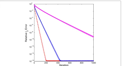
From step 1 of the algorithm, the ratio β/α plays a role of step-size of changinguk. We now investigate the performance of Algorithm 2 with various ratio β/α =
0.999
A2, 20.999A2, 40.999A2, andαis fixed. We consider the
con-figuration ofn = 215,m = n/2,s = 0.05n, the dynamic range parameterθ = 1 and the sensing matrixAis the partial DCT. The observed data is free of noise. The per-formance of Algorithm 2 in terms of the relative2error
against iteration with various values of β/α is shown in Fig. 1. As it can be seen, the performance with the largest ratioβα = 0.999A2 is the best. We therefore set
β= 0.999
A2α (19)
in our numerical experiments. In such the way,αis essen-tially the only parameter that needs to be determined. We now investigate the impact of the parameterαon the performance of Algorithm 2.
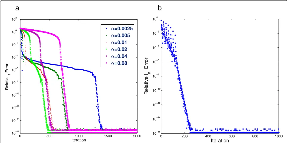
To investigate the impact of varying the parameterαon the performance of Algorithm 2, we consider the configu-rations ofn=215,m=n/2,s=0.05n, the dynamic range parameterθ =5, and the sensing matrixAis partial DCT. The observed data is noise free. Six different values ofα, namely, 0.0025, 0.005, 0.01, 0.02, 0.04, and 0.08, are tested. Figure 2a depicts the traces of the relative 1-error (see
(18)) against the number of iterations for eachα. As it can be seen from this figure, forα=0.0025, the smallest value
in our test, the relative1-error drops rapidly from 1 to
10−4, stabilizes with insignificant changes for about 1200
iterations, and then quickly drops again to the level of 10−16. Whenαincreases from 0.0025 to 0.08, the number
of iterations required for the relative 1-error dropping
from 1 to 10−4increases. Meanwhile, the numbers of iter-ations for the transitions from the first sharp jump region to the second one decrease. For example, it is about 700 forα=0.005 and only few iterations forα =0.08. These observations motivate us to extend Algorithm 2 to a sce-nario in which the parameterαcan be updated during the iteration with the goal of reducing the number of itera-tions. The proposed approach is rather simple. It begins with a relative smallαand then increases it for every given amount of iterations. A detailed flow of this new approach is given in Algorithm 3.
Algorithm 3A variant of Algorithm 1 for model(BP) Given: integersp>0,τ >1, andT>0; >0
Initialization:v0 ∈ Rm,u0 ∈ Rn,α > 0, andβ > 0 with
β
α< A12; setv−1=v0−(Au0−d0)
repeat(k≥0)
Step 1: Computeuk+1using step 1 of Algorithm 2 Step 2: Computevk+1using step 2 of Algorithm 2
Step 3: Ifkis a multiple ofpand the number of chang-ing the parametersαandβdoes not exceedT, updateα←
τα,β←τβ
untila given stopping criteria is met
0 200 400 600 800 1000 10−16
10−14 10−12 10−10 10−8 10−6 10−4 10−2 100
Iteration
Relative l
2
Error
Fig. 1The relative2error (thevertical axiswith a base 10 logarithmic scale) versus the number of iterations (thehorizontal axis) with various ratio of
β
0 500 1000 1500 2000 10−16
10−14 10−12 10−10 10−8 10−6 10−4 10−2 100 102
Iteration
Relatie l
1
Error
=0.0025 =0.005 =0.01 =0.02 =0.04 =0.08
0 200 400 600 800 1000
10−16 10−14 10−12 10−10 10−8 10−6 10−4 10−2 100
Iteration
Relative l
a
Error
a
b
Fig. 2The relative1error (thevertical axiswith a base 10 logarithmic scale) versus the number of iterations (thehorizontal axis).aConvergence of Algorithm 2 with different values ofα.bConvergence of Algorithm 3
Three new parameters introduced in Algorithm 3 are integersp > 0,τ > 1, andT > 0. The parameterT is the allowable maximum number of updating the parame-tersαandβ. For each update, the pair(α,β)will change to(τα,τβ)that will keep the ratioβ/α unchanged. The parameterpis to indicate that the underlying algorithm with a pair (α,β) will iterate p times before the algo-rithm with the pair (τα,τβ) runs another p times. We now demonstrate the efficiency of varying the parameters αandβvia applying Algorithm 3 for the same data used in Fig. 2a. We setT = 6,τ = 4, andp = 20 and ini-tializeα = mn A20Ab2
∞. Again, we chooseβ by using (19). The corresponding result is shown in Fig. 2b. It is clear to see that it takes about 200 iterations to drop the relative 1error down below 10−14. Hence, the strategy of
updat-ing the parametersαandβas described in Algorithm 3 is reasonable.
The rest of this section consists of two subsections. The first subsection focuses on comparisons of proposed algorithm to NESTA and DADM for sensing matricesA withAA = I, while the second subsection only focuses on numerical performance of proposed algorithms for random Gaussian sensing matrices.
4.1 Numerical comparisons
This subsection consists of three parts. Part one contains the comparisons of Algorithm 3, DADM, and NESTA for data setting with partial DCT measurement matrices, part two contains that for data setting with partial DWHT
measurement matrices, and part three contains results on random matrices with orthonormalized rows.
4.1.1 Numerical comparison with partial DCT sensing matrices
First of all, we compare the performance of Algorithm 3 with that of NESTA and that of DADM [23] for noise-free data. The algorithm NESTA was developed by applying a smoothing technique for the nonsmooth1-norm and
an accelerated first-order scheme, both from Nesterov’s work [19]. A parameter denoted byμis used to control how close the smoothed1-norm to the1-norm will be.
To obtain high accuracy of restored signal for NESTA, μ = 10−10 is used for partial DCT sensing matrices
and various dynamic range parameters. A parameter Tol for tolerance in NESTA varies for different values of the smoothing parameter μand different settings of gener-ated data and needs to be determined. We choose the tolerance to obtain reasonable results. We finally choose Tol = 10−12, 10−14, 10−15, respectively, for data gen-erated with dynamic range parametersθ = 1, 3, 5. For DADM, two parameters γ and β have to be predeter-mined.γ =1.618 is chosen in all settings, whileβvaries in different settings to obtain reasonable results. We choose parameters β = b1
m21, bm231, bm261 for dynamic range
and DADM is that the relative errors between the suc-cessive iterates of the reconstructed signal should satisfy the inequalityuk+1−uk/uk<Tol. We choose Tol= 10−15for data generated by partial DCT for Algorithm 3
and DADM.
For the noise-free data, the problem (BP) is used to recover underlying signals in experiments. The dimen-sions n are chosen from {213, 215} for data generated with partial DCT. The number of nonzero entries s is set to be 0.02n, 0.01n, respectively, for the number of measurements m = n/4, n/8. The performance of dif-ferent algorithms are reported in Tables 1 and 2. Based on these two tables, the performance of Algorithm 3 and DADM is comparable in terms of accuracy of recovered data for various values of dynamic range parameter θ and measurement ratio m/n. But Algorithm 3 outper-forms DADM in terms of computational cost (CUP time or iterations) for data with high value of dynamic range parameter (e.g., θ = 5). The performance of NESTA is
Table 1Numerical results with partial DCT sensing matrices for noise-free data. The number of measurementsmism=n/4, and the test signals ares-sparse withs=0.02n. Each value in a cell represents the mean over 50 trials
Method 2-error 1-error ∞-error CPU time(s) Iterations
n=213
Algorithm 3 4.99e−15 6.77e−16 6.55e−14 1.0153 387
DADM 4.48e−15 6.45e−16 5.24e−14 1.1525 391
NESTA 8.29e−11 1.75e−10 6.10e−10 1.8168 469
n=215
Algorithm 3 3.04e−15 3.81e−16 4.71e−14 5.1618 394
DADM 2.10e−15 2.96e−16 2.96e−14 5.6775 398
NESTA 8.48e−11 1.77e−10 6.80e−10 7.7550 477
n=213
Algorithm 3 6.20e−15 1.07e−15 4.65e−12 1.0640 394
DADM 3.96e−15 1.20e−15 2.72e−12 1.1331 388
NESTA 1.41e−12 4.70e−12 6.34e−10 2.8384 742
n=215
Algorithm 3 3.18e−15 5.39e−16 2.81e−12 5.3503 403
DADM 2.35e−15 3.96e−16 1.84e−12 5.7291 395
NESTA 1.48e−12 4.78e−12 6.95e−10 12.1293 748
n=213
Algorithm 3 4.69e−15 9.25e−16 2.94e−10 1.0637 397
DADM 3.01e−15 1.46e−15 1.74e−10 1.9593 665
NESTA 2.05e−14 1.96e−14 8.12e−10 4.7221 1236
n=215
Algorithm 3 3.04e−15 4.74e−16 2.08e−10 5.4653 404
DADM 2.05e−15 4.85e−16 1.28e−10 10.2053 691
NESTA 2.09e−14 3.04e−14 7.93e−10 19.5025 1209
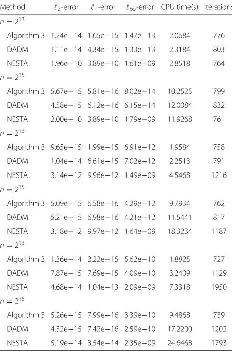
Table 2Numerical results with partial DCT sensing matrices for noise-free data. The number of measurementsmism=n/8, and the test signals ares-sparse withs=0.01n. Each value in a cell represents the mean over 50 trials
Method 2-error 1-error ∞-error CPU time(s) Iterations
n=213
Algorithm 3 1.24e−14 1.65e−15 1.47e−13 2.0684 776
DADM 1.11e−14 4.34e−15 1.33e−13 2.3184 803
NESTA 1.96e−10 3.89e−10 1.61e−09 2.8518 764
n=215
Algorithm 3 5.67e−15 5.81e−16 8.02e−14 10.2525 799
DADM 4.58e−15 6.12e−16 6.15e−14 12.0084 832
NESTA 2.00e−10 3.89e−10 1.79e−09 11.9268 761
n=213
Algorithm 3 9.65e−15 1.99e−15 6.91e−12 1.9584 758
DADM 1.04e−14 6.61e−15 7.02e−12 2.2513 791
NESTA 3.14e−12 9.96e−12 1.49e−09 4.5468 1216
n=215
Algorithm 3 5.09e−15 6.58e−16 4.29e−12 9.7934 762
DADM 5.21e−15 6.98e−16 4.21e−12 11.5441 817
NESTA 3.18e−12 9.97e−12 1.64e−09 18.3234 1187
n=213
Algorithm 3 1.36e−14 2.22e−15 5.62e−10 1.8825 727
DADM 7.87e−15 7.69e−15 4.09e−10 3.2409 1129
NESTA 4.68e−14 1.04e−13 2.09e−09 7.3318 1950
n=215
Algorithm 3 5.26e−15 7.99e−16 3.39e−10 9.4868 739
DADM 4.32e−15 7.42e−16 2.59e−10 17.2200 1202
NESTA 5.19e−14 3.54e−14 2.35e−09 24.6468 1793
inferior to that of Algorithm 3 and DADM in terms of accuracy and computational cost for various values ofθ and measurement ratio m/n. We also observe that the relative2-error and1-error of the results recovered by
Algorithm 3 along with iterations consumed are quite robust with respect to the dynamic ranges of the unknown signals.
for Algorithm 3 remains the same. For DADM, we choose parameters β = b1
m21, bm231, bm231 for dynamic range
parametersθ = 1, 3, 5, respectively, for better perfor-mance in terms of accuracy and computational cost. For the smoothing parameterμin the NESTA, we choose the default settingμ = max{0.1σ, 0.01}. The stopping crite-ria for our algorithm and DADM is that the relative errors between the successive iterates of the reconstructed signal should satisfy the inequalityuk+1−uk/uk < 10−5. And the stopping criterion for NESTA is Tol < 10−5. The performance of different algorithms are reported in Tables 3 and 4. The accuracy of recovered data from all three algorithms for each data setting is comparable. The computational cost of DADM is comparable to or slightly better than that of Algorithm 3 for data with dynamic range parameters θ = 1, 3. Both of Algorithm 3 and DADM outperform NESTA for data with dynamic range parametersθ = 1, 3 in terms of computational cost. For data with high dynamic range (e.g.,θ = 5), Algorithm 3
Table 3Numerical results with partial DCT sensing matrices for noisy data. The number of measurementsmism=n/4, and the test signals ares-sparse withs=0.02n. Each value in a cell represents the mean over 50 trials
Method 2-error 1-error ∞-error CPU time(s) Iterations
n=213
Algorithm 3 6.06e−2 6.28e−3 5.49e−1 0.2309 82
DADM 6.06e−2 6.23e−3 5.49e−1 0.2268 75
NESTA 7.25e−2 2.47e−2 6.68e−1 0.4006 123
n=215
Algorithm 3 6.10e−2 6.28e−3 6.15e−1 1.0700 80
DADM 6.10e−2 6.23e−3 6.15e−1 1.0925 76
NESTA 7.23e−2 2.29e−2 7.14e−1 1.7906 123
n=213
Algorithm 3 1.90e−2 1.76e−3 10.0453 0.2684 99
DADM 1.89e−2 1.72e−3 10.0370 0.2181 71
NESTA 2.05e−2 1.61e−2 12.0646 0.4353 132
n=215
Algorithm 3 1.88e−2 1.60e−3 11.3331 1.5018 111
DADM 1.88e−2 1.54e−3 11.3232 1.0662 71
NESTA 2.09e−2 1.54e−2 13.0586 1.8931 132
n=213
Algorithm 3 1.13e−3 1.03e−4 49.7915 0.2740 101
DADM 1.13e−3 5.85e−4 50.3671 0.5953 199
NESTA 1.28e−3 1.13e−3 61.2107 0.4243 125
n=215
Algorithm 3 1.18e−3 5.73e−5 56.1854 1.3543 102
DADM 1.18e−3 5.49e−4 56.8402 2.9696 200
NESTA 1.34e−3 1.11e−3 66.0787 1.7721 126
Table 4Numerical results with partial DCT sensing matrices for noisy data. The number of measurementsmism=n/8, and the test signals ares-sparse withs=0.01n. Each value in a cell represents the mean over 50 trials
Method 2-error 1-error ∞-error CPU time(s) Iterations
n=213
Algorithm 3 1.02e−1 1.94e−2 8.48e−1 0.3296 122
DADM 1.02e−1 1.94e−2 8.48e−1 0.2790 94
NESTA 1.20e−1 3.07e−2 1.0099 0.4606 145
n=215
Algorithm 3 1.02e−1 1.83e−2 9.37e−1 1.5691 121
DADM 1.02e−1 1.82e−2 9.37e−1 1.4009 95
NESTA 1.22e−1 2.74e−2 1.1065 2.0506 149
n=213
Algorithm 3 2.97e−2 5.30e−3 15.1517 0.2853 102
DADM 2.97e−2 5.21e−3 15.1429 0.3028 99
NESTA 3.10e−2 2.08e−2 17.2106 0.5012 160
n=215
Algorithm 3 2.92e−2 5.89e−3 16.8347 1.5609 120
DADM 2.92e−2 5.79e−3 16.8203 1.4675 99
NESTA 3.16e−2 1.93e−2 19.4426 2.2300 160
n=213
Algorithm 3 1.94e−3 2.87e−4 75.5390 0.3231 115
DADM 1.92e−3 3.49e−4 75.4992 0.6975 230
NESTA 1.93e−3 1.50e−3 90.2023 0.4981 157
n=215
Algorithm 3 1.89e−3 2.00e−4 86.3350 1.5025 114
DADM 1.88e−3 2.06e−4 86.2110 3.3468 233
NESTA 2.03e−3 1.41e−3 99.4225 2.2662 158
performs the best in terms of computational cost while DADM performs the worst.
4.1.2 Numerical comparison with partial DWHT sensing matrices
The performance of the three algorithms will be discussed in this part. The performance of the algorithms will be presented in a different manner from the previous part with partial DCT sensing matrices. In all of those three algorithms, the computational cost is mainly attributed to the matrix-vector multiplication involving A or A. Under the assumption that AA = I, the three algo-rithms only have two such multiplications, one involving A and the other involvingA in each iteration. Hence, we will only use the number of iterations to represent the computational cost. For the accuracy, only the relative 2− error will be selected. The setting of parameters of
300 350 400 450 500 550 600 650 700 750 10−15
10−14 10−13 10−12 10−11 10−10 10−9
Iteration (n=2048, m=n/4)
Relative l
2
−Error
Alg. 3, =1 Alg. 3, =3 Alg. 3, =5 DADM, =1 DADM, =3 DADM, =5 NESTA, =1 NESTA, =3 NESTA, =5
60 80 100 120 140 160 180
10−3 10−2 10−1
Iteration (n=2048, m=n/4)
Releative l
2
Error
Alg. 3, =1 Alg. 3, =3 Alg. 3, =5 DADM, =1 DADM, =3 DADM, =5 NESTA, =1 NESTA, =3 NESTA, =5
a
b
Fig. 3Numerical results with partial DWHT sensing matrices. The relative2errors (thevertical axiswith base 10 logarithmic scale) versus the iteration consumed (thehorizontal axis) forathe noise-free case andbthe noise case (the right). The colorsred,blue, andyellowrepresent the dynamic ranges of the tested signals withθbeing 1, 3, and 5, respectively
μ = 10−8, Tol= 10−13 is used in NESTA for noise-free data with dynamic range parameterθ =5.
Figure 3 shows the results of Algorithm 3, DADM, and NESTA when the dimension of the tested signals n is 2048 and the number of measurements m is n/4. The
symbols “,” “♦,” and “∇” denote the results produced by Algorithm 3, DADM, and NESTA, respectively. The colors “red,” “blue,” and “yellow” represent the dynamic ranges of the tested signals withθbeing 1, 3, and 5, respec-tively. The relative 2-error is displayed with a base 10
300 350 400 450 500 550 600 10−14
10−13 10−12
Iteration (n=2048, m=n/4)
Relative l
2
Error
Alg. 3, =1 Alg. 3, =3 Alg. 3, =5 DADM, =1 DADM, =3 DADM, =5
60 80 100 120 140 160 180 10−3
10−2 10−1
Iteration (n=2048, m=n/4)
Relative l
2
Error
Alg. 3, =1 Alg. 3, =3 Alg. 3, =5 DADM, =1 DADM, =1 DADM, =1
a
b
Table 5Numerical results with Gaussian measurement matrices for noise-free data. The test signals have sizen=4096. Each value in a cell represents the mean over 50 trials
m s θ 2-error 1-error ∞-error CPU time(s) Iterations
n/4 0.02n 1 1.64e−13 2.31e−14 2.07e−12 6.0768 844
n/8 0.01n 1 3.28e−13 4.93e−14 3.70e−12 5.1040 1305
n/4 0.02n 3 1.32e−13 3.13e−14 9.93e−11 5.7287 799
n/8 0.01n 3 3.93e−13 1.06e−13 2.61e−10 4.9531 1255
n/4 0.02n 5 1.08e−13 2.55e−14 5.76e−09 5.3643 752
n/8 0.01n 5 4.01e−13 1.25e−13 2.10e−08 4.5700 1157
logarithmic scale plot for the vertical axis. We see clearly that performance of the three algorithms follows the simi-lar phenomena that was seen in the numerical results with partial DCT measurements. The same conclusions can be drown for the results withm=n/8 as well.
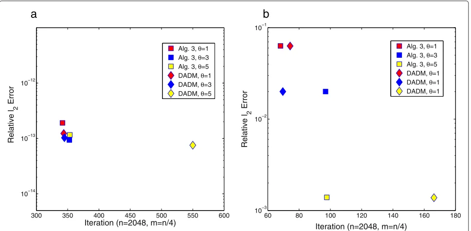
4.1.3 Numerical comparison with orthonormal Gaussian sensing matrices
In this part, the comparisons of numerical results with orthonormal Gaussian sensing matrices will be shown. Due to the unavailability of source code of NESTA for such sensing matrices, only the comparison between Algorithm 3 and DADM is provided. The setting of parameters of Algorithms 3 and DADM are the same as above except that the stopping criterion Tol=10−14is used for noise-free data. The numerical result is reported in Fig. 4 in the same manner as in previous part with DWHT sensing matrices. For the noise-free data or noisy data, the perfor-mance of Algorithm 3 and DADM is comparable in terms of relative2error. For noise-free data, the performance
of Algorithm 3 and DADM is comparable only for data with dynamic range parametersθ =1, 3 in terms of com-putational cost; while Algorithm 3 outperforms DADM in terms of computational cost (e.g., iteration) for data withθ =5. For noisy data and in terms of computational cost, performance of the two algorithms is comparable for θ = 1; DADM performs slightly better than Algorithm 3 forθ = 3; and Algorithm 3 outperforms DADM for θ =5. The same conclusions can be drawn for the results withm=n/8 as well.
4.2 Simulation with Gaussian sensing matrices
In this subsection, we only focus on the simulation of Algorithm 3 for data generated by general Gaussian sens-ing matrices (e.g., rows are not orthonormal), that is, AA =I. In such scenario, we do not compare Algorithm 3 with NESTA and DADM since the available source code of NESTA does not apply, and DADM needs an inner loop in each of iteration. The setting of parameters for Algorithm 3 is the same as the setting for data with orthonormal Gaussian sensing matrices. The results for noise-free data and noisy data are reported in Tables 5 and 6, respectively. It can be seen that the underlying signal can be recovered with high accuracy for noise-free data and with reasonable high accuracy for noisy data.
5 Conclusions
We reformulated the 1-norm minimization problems
(BP) and(BP) via indicator functions as unconstrained minimization problems. The objective function for each unconstrained problem is the sum of the1-norm of the
underlying signaluand the indicator function of a set in Rm, which is {0} for (BP) or the -ball for(BP
), com-posing with the affine transformation Au− b. Due to the structure of this objective function and the availabil-ity of the explicit forms of the proximavailabil-ity operators for both the 1-norm and the indicator function, an
accu-rate and efficient algorithm is developed for recovering sparse signals based on fixed-point equation. The algo-rithm outperforms NESTA in terms of the relative2, the
relative1, and the absolute∞error measures as well as
Table 6Numerical results with Gaussian measurement matrices for noisy data. The test signals have sizen=4096. Each value in a cell represents the mean over 50 trials
m s θ 2-error 1-error ∞-error CPU time(s) Iterations
n/4 0.02n 1 1.01e−3 4.08e−4 8.99e−3 2.3762 315
n/8 0.01n 1 1.65e−3 5.13e−4 1.29e−2 1.8412 455
n/4 0.02n 3 3.57e−4 1.68e−4 0.1729 1.2184 160
n/8 0.01n 3 6.10e−4 2.46e−4 0.2602 0.8990 211
n/4 0.02n 5 4.51e−05 5.52e−05 2.1526 1.0484 139
the computational cost for tested signals ranging from a low dynamic range to a high dynamic range with different sizes. For signal with high dynamic range, the proposed algorithm also outperforms DADM in terms of compu-tational cost but yields comparable accuracy. Further, the proposed algorithms also solve general problems without requiring conditionAA=Iefficiently and accurately.
Competing interests
The authors declare that they have no competing interests.
Acknowledgements
Lixin Shen was partially supported by the US National Science Foundation under grant DMS-1115523 and by an award from National Research Council via the Air Force Office of Scientific Research. Yuesheng Xu was partially supported by the US National Science Foundation under grant DMS-1115523.
Received: 9 April 2015 Accepted: 13 July 2015
References
1. E Candes, J Romberg, T Tao, Stable signal recovery from incomplete and inaccurate measurements. Commun. Pur. Appl. Math.59(8), 1207–1223 (2006)
2. E Candes, T Tao, Near optimal signal recovery from random projections: universal encoding strategies? IEEE Trans. Inf. Theory.52(12), 5406–5425 (2006)
3. SS Chen, DL Donoho, MA Saunders, Atomic decomposition by basis pursuit. SIAM J. Sci. Comput.20, 33–61 (1998)
4. SJ Wright,Primal-Dual Interior-Point Methods. (Society for Industrial and Applied Mathematics (SIAM), Philadelphia, PA, 1997)
5. P Combettes, V Wajs, Signal recovery by proximal forward-backward splitting. Multiscale Model. Simul. A SIAM Interdiscip. J.4, 1168–1200 (2005)
6. MAT Figueiredo, SJ Wright, RD Nowak, Gradient projection for sparse reconstruction: applications to compressed sensing and other inverse problems. IEEE J. Selected Topics Signal Process.1, 586–597 (2007) 7. A Beck, M Teboulle, A fast iterative shrinkage-thresholding algorithm for
linear inverse problems. SIAM J. Imaging Sci.2, 183–202 (2009) 8. ET Hale, W Yin, Y Zhang, Fixed-point continuation for1minimization:
methodology and convergence. SIAM J. Optim.19, 1107–1130 (2008) 9. J-F Cai, S Osher, Z Shen, Split Bregman methods and frame based image
restoration. Multiscale Model. Simul.: A SIAM Interdiscip. J.2, 337–369 (2009)
10. W Yin, S Osher, D Goldfarb, J Darbon, Bregman iterative algorithms for1
minimization with applications to compressed sensing. SIAM J. Imaging Sci.1, 143–168 (2008)
11. A Chambolle, RA DeVore, N-Y Lee, BJ Lucier, Nonlinear wavelet image processing: variational problems, compression, and noise removal through wavelet shrinkage. IEEE Trans. Image Process.7, 319–335 (1998) 12. R Chan, T Chan, L Shen, Z Shen, Wavelet algorithms for high-resolution
image reconstruction. SIAM J. Sci. Comput.24(4), 1408–1432 (2003) 13. B Efron, T Hastie, I Johnstone, R Tibshirani, Least angle regression. Ann.
Stat.32, 407–451 (2004)
14. MR Osborne, B Presnell, BA Turlach, A new approach to variable selection in least squares problems. IMA J. Numeric. Anal.20, 389–403 (2000) 15. D Donoho, Y Tsaig, Fast solution of1-norm minimization problems
when the solution may be sparse. IEEE Trans. Inf. Theory.54(11), 4789–4812 (2008)
16. E van den Berg, MP Friedlander, Probing the Pareto frontier for basis pursuit solutions. SIAM J. Scie. Comput.31, 890–912 (2008)
17. RT Rockafellar,Convex Analysis. (Princeton University Press, Princeton, NJ, 1970)
18. S Becker, J Bobin, E Candes, NESTA: a fast and accurate first-order method for sparse recovery. SIAM J. Imaging Sci.4(1), 1–39 (2009)
19. Y Nesterov, Smooth minimization of non-smooth functions. Mathematical Programming, Series A.103, 127–152 (2005)
20. Q Li, CA Micchelli, L Shen, Y Xu, A proximity algorithm accelerated by Gauss-Seidel iterations forL1/TVdenoising models. Inverse Probl. 28, 095003 (2012)
21. CA Micchelli, L Shen, Y Xu, Proximity algorithms for image models: denoising. Inverse Probl.27, 045009–30 (2011)
22. CA Micchelli, L Shen, Y Xu, X Zeng, Proximity algorithms for the L1/TV image denoising model. Adv. Comput. Math.38, 401–426 (2013) 23. J Yang, Y Zhang, Alternating direction algorithms for l1-problems in
compressive sensing. SIAM J. Scie. Comput.33, 250–278 (2011) 24. W Deng, W Yin, On the global and linear convergence of the generalized
alternating direction method of multipliers (ADMM). Technical report, UCLA, Center for Applied Mathematics (2012)
25. X Zhang, M Burger, S Osher, A unified primal-dual algorithm framework based on Bregman iteration. J. Sci. Comput.46, 20–46 (2011)
26. S Boyd, N Parikh, E Chu, B Peleato, J Eckstein, Distributed optimization and statistical learning via alternating direction method of multipliers. Foundations Trends Mach. Learn.3, 1–122 (2010)
27. A Chambolle, T Pock, A first-order primal-dual algorithm for convex problems with applications to imaging. J. Math. Imaging Vis.40, 120–145 (2011)
Submit your manuscript to a
journal and benefi t from:
7Convenient online submission
7Rigorous peer review
7Immediate publication on acceptance
7Open access: articles freely available online
7High visibility within the fi eld
7Retaining the copyright to your article