Performance Analysis of Optical Burst Switched Networks with Dynamic Simultaneous Link Possession

(1)

TZVETELINA (LINA) BATTESTILLI Performance Analysis of Optical Burst Switched Networks with Dynamic Simultaneous Link Possession. (Under the direction of Professor HARRY G. PERROS).

Given the current state of the technology, the Optical Burst Switched (OBS) architecture is a practical optical switching solution for the optical networks. In OBS, the user data is transmitted in variable size data units, called bursts, which travel as an optical signal along the entire route. The control information for each burst is transmitted prior to its corresponding burst and it is electronically processed at each hop along the route. The dynamic nature of OBS allows for network adaptability and scalability, which makes it very suitable for the transmission of bursty traffic.

In this thesis we study and analyze the performance of OBS networks. We consider the case when the bursts are large enough to simultaneously hold wavelengths on multiple links along the route. Since the size of the bursts varies and the link distance between two adjacent network nodes also varies, a burst may simultaneously occupy wavelengths on a variable number of links as it travels from its source to its destination. As the burst propagates through the network, it dynamically acquires and releases wavelengths from link to link. In this thesis, we propose queueing network models that feature dynamic simultaneous link possession and analyze them in order to obtain the end-to-end burst loss probabilities.

(2)

Performance Analysis of Optical Burst Switched Networks with Dynamic Simultaneous Link Possession

by

Tzvetelina Battestilli

B.S. Electrical Engineering, M.S. Computer Networking

A dissertation submitted to the Graduate Faculty of North Carolina State University

in partial satisfaction of the requirements for the Degree of

Doctor of Philosophy

Department of Computer Science

Raleigh

2005

Approved By:

Dr. Arne Nilsson Dr. Yannis Viniotis

Dr. Harry Perros Dr. William Stewart

(3)

(4)

iii

Biography

(5)

Acknowledgements

I would like to thank my adviser Dr. Harry G. Perros for his guidance and encouragement during the process of writing this thesis. He was supportive, insightful and always available to meet with me and discuss my progress. I thank him for introducing me to the interesting world of queueing theory. I very much enjoyed our weekly meetings.

I would like to acknowledge Dr. Nilsson, Dr. Stewart and Dr. Viniotis for agreeing to be on my thesis committee and for their valuable advise and recommendations.

I especially want to thank my wonderful husband for his unconditional support during my graduate studies. I want to thank him for listening to me and living with me when I got really involved in my research. I also want to thank him for the last six months, when he took care of our newborn son each evening and all weekend long while I was finishing this thesis.

(6)

v

List of Figures

1.1 Optical Network Evolution . . . 2

1.2 OBS Network Architecture . . . 3

1.3 One-Way Signaling Scheme . . . 5

1.4 Reservation and Release Schemes in OBS . . . 9

1.5 Control and Data Planes in Jumpstart . . . 10

2.1 A Path in an OBS Network . . . 18

2.2 Bursts simultaneously hold wavelengths on multiple links . . . 19

2.3 Queueing Model for an OBS Network with Simultaneous Link Possession . 20 3.1 The Queueing network model for an OBS Path, where the bursts span two links . . . 24

3.2 Bursts simultaneously hold wavelengths on two links . . . 25

3.3 Multiplexed IDLE-ON Sources . . . 26

3.4 Queueing Network for an OBS path of 6 links with 2 wavelengths per link . 35 3.5 Burst Loss Probability for W=16, L=8, N=32, low to high load . . . 40

3.6 Utilization λ/(µW) for W=16, L=8, N=32, low to high load . . . 40

3.7 Burst Loss Probability for W=8, L=6, N=16, low to moderate load . . . . 41

3.8 Utilization λ/(µW) for W=8, L=6, N=16, low to moderate load . . . 41

3.9 State-Dependent Arrival Rates for W=16, α= 0.2,γ = 0 . . . 42

3.10 Burst Loss Probability for W=16, L=8,γ = 0.5,N=32 and α= 0.5 . . . 44

3.11 The Queueing network model for an OBS path, where the bursts span either one or two links . . . 46

3.12 Bursts simultaneously hold wavelengths on either one or two links . . . 47

3.13 Multiplexed IDLE-SHORT-LONG Sources . . . 49

3.14 Queueing Network for an OBS path of 4 links with 2 wavelengths per link . 51 3.15 Low Load, Short Bursts, W=8, K=6, N=16,γ = 1 . . . 62

3.16 Low Load, Long Bursts, W=8, K=6, N=16, γ = 1 . . . 62

3.17 Low Load, Avg. Wavelength Utilization, W=8, K=6, N=16, γ = 1 . . . 63

3.18 High Load, Short Bursts, W=10, K=6, N=16, γ = 1 . . . 65

3.19 High Load, Long Bursts, W=10, K=6, N=16, γ = 1 . . . 65

(9)

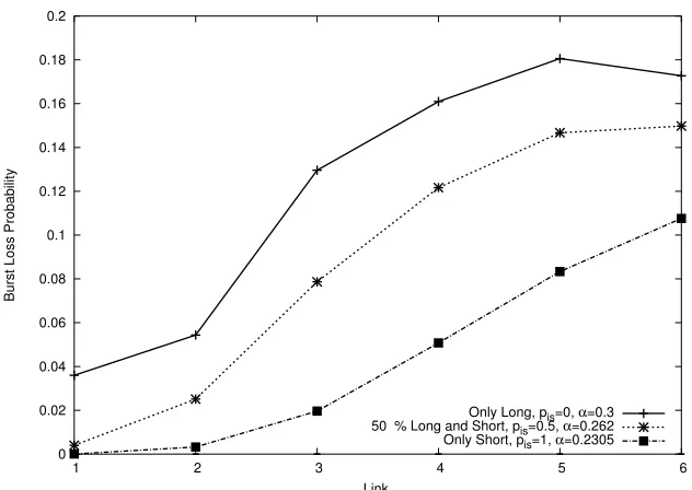
3.21 Loss Probability while varying the mixture of Short and Long Bursts, W=16,

K=6, N=32, γ = 2 . . . 67

3.22 Utilization while varying the mixture of Short and Long Bursts, W=16, K=6, N=32,γ = 2 . . . 67

4.1 Queueing Network Model of an OBS path with K links with short and long bursts arriving as a Poisson process . . . 71

4.2 State Transition Modified Rate Diagram for Short Nodes . . . 73

4.3 State Transition Modified Rate Diagram for Long Bursts . . . 75

4.4 Short Burst Loss Probability, W=50, K=7, γ = 20,Psh = 1 . . . 81

4.5 Long Burst Loss Probability, W=50, K=7,γ = 20, Psh= 0 . . . 81

4.6 Short Burst Loss Probability, W=50, K=7, γ = 20,Psh = 0.25 . . . 81

4.7 Long Burst Loss Probability, W=50, K=7,γ = 20, Psh= 0.25 . . . 81

4.9 Long Burst Loss Probability, W=50, K=7,γ = 20, Psh= 0.5 . . . 81

4.11 Long Burst Loss Probability, W=50, K=7, γ = 20, Psh= 0.75 . . . 82

4.12 Short Burst Loss Probability, W=100, K=7, γ = 50,Psh= 1 . . . 82

4.13 Long Burst Loss Probability, W=100, K=7, γ= 50, Psh = 0 . . . 82

4.14 Short Burst Loss Probability, W=100, K=7, γ = 50,Psh= 0.25 . . . 82

4.15 Long Burst Loss Probability, W=100, K=7, γ= 50, Psh = 0.25 . . . 82

4.17 Long Burst Loss Probability, W=100, K=7, γ = 50, Psh = 0.5 . . . 83

4.20 Short Burst Loss Probability, W=200, K=7, γ = 100, Psh= 1 . . . 83

4.21 Long Burst Loss Probability, W=200, K=7, γ = 100, Psh = 0 . . . 83

4.22 Short Burst Loss Probability, W=200, K=7, γ = 100, Psh= 0.25 . . . 84

5.1 Interrupted Poisson Process . . . 88

5.2 Blocking Probability as a function of r andc2 . . . 91

5.3 Departure Process from an IPP loss node . . . 93

5.4 Transition Rate Diagram for pa,w,c . . . 94

5.5 Transition Rate Diagram for an IPP loss node . . . 97

5.6 Overflow System . . . 98

5.7 Transformation of an IPP-node to an ERM-node . . . 100

5.8 ERM Transformation for each node of the OBS path . . . 101

(10)

ix

5.11 Blocking Probability for W=50, λcrossavg = 45,λlocalavg = 10, r= 0.6 . . . 109 5.12 Blocking Probability for W=200, λcross_avg = 180, λlocal_avg = 40,r = 0.6 . . . 110 5.13 Blocking Probability for W=500, λcross

avg = 450, λlocalavg = 100,r = 0.6 . . . 111 5.14 Blocking Probability for W=50, λcross

avg = 45,λlocalavg = 10, c2 = 20 . . . 112 5.15 Blocking Probability for W=200, λcross

avg = 180, λlocalavg = 40,c2 = 20 . . . 113 5.16 Blocking Probability for W=500, λcross

(11)

List of Tables

3.1 Possible State Transitions for sub-systemswhen in state (ni−₁,i, ni,i+1, ni+1,i+2)

30

3.2 Possible State Transitions for sub-systemswhen in state (ni−1,i, ni, ni,i+1, ni+1)

54

3.3 Low Load, Relative % Error . . . 64 3.4 High Load, Relative % Error . . . 64

4.1 Burst Loss Probabilities for an OBS Path with K = 3 Links, W = 2 Wave-lengths, Cross Mean ratesλ1= 1 andλ01= 1, Local Mean Rates γs = 1 and

γl= 1 . . . 80 4.2 Maximum Relative Errors . . . 85 4.3 Number of Iterations . . . 86

(12)

xi

List of Algorithms

1 Sub-System Decomposition Algorithm for a Queueing Network, where the bursts span two links . . . 33 2 Sub-System Decomposition Algorithm for a Queueing Network, where the

bursts span one or two links . . . 56 3 Single-Node Decomposition Algorithm for a Queueing Network where the

Bursts Span One or Two Links and a Large Number of Wavelengths . . . 77 4 Equivalent Transformation Algorithm for a Queueing Network With Bursty

(13)

Chapter 1

Introduction

1.1 Classification of All-Optical Networks

The potential of optical fiber was fully realized with the invention of dense wave-length division multiplexing (WDM). The evolution of WDM optical networks can be clas-sified as shown in Figure 1.1. Current WDM networks operate over point-to-point links, where optical-to-electrical-to-optical (OEO) conversion is required at each step. Future WDM designs focus on All-Optical Networks (AON) where the user data travels entirely in the optical domain. The elimination of the OEO conversion in AONs allows for un-precedented transmission rates. AONs can further be categorized as wavelength-routed networks (WRN), optical burst switched networks (OBSN) or optical packet switched net-works (OPSN). Also, each step of the optical evolution begins with a simpler ring design before moving on to the more general mesh topologies. In the following paragraphs we briefly outline the pros and cons of future all-optical architectures.

(14)

2

Wavelength−Routed Ring Point−to−Point WDM Links

Optical Network Functionality

Optical Packet Switched Optical Burst Switched Mesh Optical Burst Switched Ring Wavelength−Routed Mesh

time

AONs

OEO required

Figure 1.1: Optical Network Evolution

of routing and wavelength allocation of the lightpaths in order to optimally satisfy the user traffic. Another challenge for WRNs is their quasi-static nature, which prevents them from efficiently supporting constantly changing user traffic. The proposed signaling protocol for WRNs is the Generalized Multi-Protocol Label Switching (GMPLS) [1].

The most sophisticated AON is the OPSN [2], where the user traffic is carried in optical packets along with in-band control information. The control info is extracted and electronically processed at each node. The OPSN is a desirable architecture because it is a well-known fact that electronic packet switched networks are characterized by high through-put and easy adaptation to congestion or failure. The problem with OPSNs, however, is the lack of practical optical buffer technology .

(15)

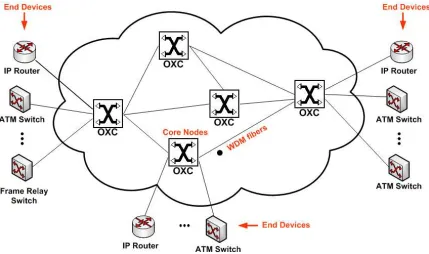
Figure 1.2: OBS Network Architecture

for the transmission of Internet traffic. In this thesis we study and analyze the performance of OBS networks. Even though the term OBS is used to describe a variety of architectures and protocols [5], we describe its definitive characteristics in the following section.

1.2 Optical Burst Switching

An OBS network consists of core nodes and end-devices interconnected by WDM fibers as shown in Figure 1.2. An OBS core node consists of an optical cross connect (OXC), an electronic switch control unit, and routing and signaling processors [6]. An OXC is a non-blocking switch that can switch an optical signal from an input port to an output port without converting the signal to electronics. The OBS end-devices are equipped with an OBS interface and could be electronic IP routers, ATM switches, frame relay switches, etc. Each OBS end-device is connected to an ingress OBS core node.

(16)

4

assembles it into larger variable-size units, called bursts. For each burst, the end-device also constructs a control packet, which contains information about the burst, such as the burst length, burst destination address, etc. This control packet is immediately sent along the route of the burst and it is electronically processed at each node. The function of the control packet is to inform the nodes of the impending data burst and to set up an end-to-end optical path between the source and the destination. After a delay time, known as the offset, the end-device transmits the burst itself. The burst travels as an optical signal over the end-to-end optical path set up by its control packet. This optical path is torn down after the burst transmission is completed.

This separation of the control information and the burst data is one of the main advantages of OBS. It facilitates efficient electronic control while it allows for a great flexi-bility in the format and transmission rate of the user data. This is because the bursts are transmitted entirely as an optical signal, which remains transparent throughout the net-work. In general, the time it takes the control packet to reach the destination end-device is equal to the end-to-end propagation delay plus the sum of all the processing delays at all the intermediate core nodes. On the other hand, the time it takes for a burst to reach the destination end-device is only equal to the end-to-end propagation delay. The reason is that the burst is transmitted as an optical signal that goes through the OBS switches without any processing or buffering delays. The transmission of a burst is delayed by an offset so that it always arrives at an OBS node, after its switch control unit has had the chance to process the control packet associated with the burst and configure its optical switch fabric. The offset, therefore, is a function of the number of hops that the control packet has to traverse end-to-end.

Burst aggregation algorithm

(17)

Figure 1.3: One-Way Signaling Scheme

and cause the unfair loss of other bursts. The minimum burst length is necessary because very short bursts may give rise to too many control packets. This situation can overload the control unit of the OBS node. The burst aggregation algorithm may use bit-padding if there is not enough data to assemble a minimum size burst.

One way to provide classes of traffic in OBS is to implement priority queues at the edge of the network during the burst aggregation. Based on the class of service, the end-devices sort the upper layer traffic into different queues [7]. As a result, each end-device will have C*N priority queues, where C is the number of service classes and N is the number of possible destinations. An appropriate scheduling algorithm guarantees that these queues are served according to their priority.

Signaling, routing and wavelength allocation

(18)

6

time line so as to show the actions taken by each node. End-device A transmits a control packet to its ingress OBS node. The control packet is processed at the ingress node. If the connection can be accepted, it is forwarded to the next node. The control packet is received by the next OBS node, and is processed. Assuming that the node can accept the connection, it is forwarded to the destination end-device. In the mean time, after an offset delay, end-device A starts transmitting the burst, which is propagated through the two OBS nodes to the end-device B as an optical signal without any buffering. In this example, the transmission of the burst begins before the control packet had reached the destination.

Note that in a one-way signaling scheme, it is possible that a burst may be lost if the control packet is not able to reserve resources at any of the OBS nodes along the bursts route. The OBS architecture, however, does not retransmit lost bursts as this job is left to the upper protocol layers. Note also, that it is very important that the offset is calculated correctly. If the offset is too short, then the burst may arrive at a node prior to the control packet and thus be lost. On the other hand, offsets that are too long reduce the throughput of the end-device.

Due to this one-way signaling scheme and lack of buffers, burst loss may occur in the OBS network. That is, the control packets may be unsuccessful at reserving resources at some of the intermediate OBS nodes. Bufferless transmission is important in OBS because electronic buffers require optical-to-electrical-to-optical conversion, which slows down the transmission while optical buffers are still quite impractical. In fact, as of today, there is no practical way to buffer light and the only possible optical buffering is to delay the signal through very long fiber delay lines (FDLs). The use of FDLs could potentially improve the network throughput [8, 9, 10]. However, the FDL technology is still being developed and it is not a viable solution yet. Another interesting strategy to reduce the burst loss in OBS is deflection routing. In case of resource contention at an output port of an OBS node, a burst is not dropped but instead it is re-routed on an alternative path to its destination [11, 12, 13]. An OBS network also needs an effective routing algorithm. One approach is to route the bursts on a hop-by-hop basis, as in an IP network, using a fast table look-up algorithm to determine the next hop. Another approach is to use multi-protocol label switching (MPLS) [14]. The MPLS idea is to assign the control packets to forward equivalent classes (FECs) at the OBS end-devices in order to reduce the processing of the routing info to the time it takes to swap the labels. A third approach is to use explicitly pre-calculated

(19)

RSVP-TE. Explicit routing is very useful in a constrained-based routed OBS network, where the traffic routes have to meet certain QoS metrics such as delay, hop-count, BER or bandwidth. In addition, in order to deal with node or link failures, OBS routing should also be augmented with a fast protection and restoration schemes. Unfortunately, this is a weak point for explicit routing schemes because sometimes the routing tables may become outdated due to the long propagation time until a failure message reaches all of the OBS nodes. The OBS protection and restoration schemes are still an open problem.

As in any other type of optical network, each OBS network has to assign wave-lengths at the different WDM fibers along the burst route. This wavelength allocation in OBS depends on whether or not the network is equipped with wavelength converters, which are devices that optically convert signals from one wavelength to another. In an OBS net-work with no wavelength converters, the entire path from the source to the destination is constrained to using the same wavelength. With a wavelength conversion capability at each OBS node, if two bursts contend for the same wavelength on the same output port, then the OBS node may optically convert one of the signals from an incoming wavelength to a different outgoing wavelength. Wavelength conversion is a desirable characteristic in an OBS network as it reduces the burst loss probability; however, it is still an expensive tech-nology. An OBS network will most likely be sparsely equipped with wavelength converters, i.e., only certain critical nodes will have that ability.

(20)

8

Reservation and Release of Resources

Upon receipt of a control packet, an OBS node processes the included burst infor-mation. It also allocates resources in its switch fabric that will permit the incoming burst to be switched out on an output port toward the destination. Baldine et. al [16] classify the resource reservation and release schemes in OBS based on the amount of time a burst occupies a path inside the switching fabric of an OBS node.

There are two OBS resource reservation schemes, namely, immediate reservation and delayed reservation. In the immediate reservation scheme, the control unit configures the switch fabric to switch the burst to the correct output port immediately after it has processed the control packet. In the delayed reservation scheme, the control unit uses the the offset parameter to calculate the time of arrival tb of the burst at the node, and it configures the switch fabric at tb.

There are also two different resource release schemes, namely, timed release and explicit release. In the timed-release scheme, the control unit uses the burst length infor-mation to calculate when the burst will completely go through the switch fabric. When this time occurs, it instructs the switch fabric to release the allocated resources. This requires knowledge of the burst duration. An alternative scheme is the explicit release scheme, where the transmitting end-device sends a release message to inform the OBS nodes along the path of the burst that it has finished its transmission. The control unit instructs the switch fabric to release the connection when it receives this message.

Combining the two reservation schemes with the two release schemes results in the following four possibilities: immediate reservation/explicit release, immediate reser-vation/timed release, delayed reservation/explicit release and delayed reserreser-vation/timed release, see Figure 1.4. Each of these schemes has advantages and disadvantages.

(21)

Figure 1.4: Reservation and Release Schemes in OBS

loss.

In the OBS literature, the three most popular OBS variants are Just-In-Time (JIT) [17], Just-Enough-Time (JET) [3] and Horizon [18]. They mainly differ based on their wavelength reservation schemes. The JIT protocol utilizes the immediate reservation scheme while the JET protocol uses the delayed reservation scheme. The Horizon reservation scheme can be classified as somewhere between immediate and delayed. In Horizon, upon receipt of the control packet, the control unit scheduler assigns the wavelength whose deadline (horizon) to become free is closest to the time before the burst arrives.

An OBS Testbed

The OBS technology is still in the developmental stage and it has not been stan-dardized yet. So far, OBS has mostly been studied through simulation. Recently, however, researchers from MCNC Research and Development Institute and North Carolina State University (NCSU) jointly designed an OBS architecture, based on the JIT protocol. Their OBS project is called Jumpstart [17]. Its architecture and signaling definition are detailed enough to begin a standardization path.

(22)

10

(23)

the control plane and the data plane. The data plane is responsible for the transportation of the bursts as optical signals while the control plane is responsible for the signaling, routing and network management (See Figure 1.5). The control plane could be either logical (designating one of the wavelengths in the all-optical network to be exclusively used by the control traffic) or it could be a completely separate electrical network, such as an ATM for example.

In Jumpstart, there are two types of connections: on-the-fly and persistent. The on-the-fly connections are set up and torn down each time an end-device wants to transmit a burst. Therefore, as the routing information in the network changes, the path between a source-destination pair may change. If, however, it is necessary to transmit a series of bursts over the same route, then it is possible to set up a persistent connection.

The scientists at MCNC and NCSU also designed and prototyped a JIT protocol accelerator card (JITPAC). This card handles the control information in the Jumpstart network. The JITPAC includes a microprocessor and a Field Programmable Gate Array (FPGA) connected via a 64-bit bus. To assure fast connection provisioning, the JITPAC uses the FPGA and implements in hardware the establishment and the tear down of con-nections, i.e., the processing of signaling messages. All the other control functions are implemented in software, running on the microprocessor. The JITPACs communicate with each other via an ATM network.

In Jumpstart, the addressing scheme is hierarchical with variable length addresses similar to the NSAP address format. The hierarchical addressing scheme allows different administrative entities to be responsible for assigning their part of the address and deciding how to further subdivide the address space.

Because of the nature of OBS, the signaling messages must follow the same path as their corresponding bursts in order to set up or tear down optical connections. This constraint is not necessary for the other control messages, such as those used to exchange routing information or report network failures. In Jumpstart, there are two different routing architectures: 1) for the data plane and the signaling messages, and 2) for the remaining control messages. This design decision was made to reduce the complexity of implementation and use existing routing protocols whenever appropriate, especially in the control plane.

(24)

12

route computation is centralized and it is done at the Routing Data Node (RDN), a server attached to one of the JITPACs. Each JITPAC collects information about the outgoing optical interfaces of its OXC. This includes optical QoS information such as the linear and non-linear impairments of the fibers. This information is sent to the RDN, which computes the data paths between all pairs of OBS nodes and downloads that information back to the JITPACs.

In January 2004, the researchers built a Jumpstart testbed within the US Gov-ernment’s Advanced Technology Demonstration Network (ATDnet) in the Washington DC area. They demonstrated its performance by transporting uncompressed digital HDTV signals. The demonstration confirmed that the Jumpstart optical connection establishment time is only a few milliseconds through micro-electro-mechanical switches (MEMS). This time can be reduced to mere microseconds if faster photonic switches replace the MEMS and the FPGAs in the JITPACs are replaced by Application Specific Integrated Circuits (ASICs). This connection provisioning time is a significant improvement over GMPLS, which promises connection establishment within minutes, or the weeks and even months that it currently takes for a manual set up.

With its fast connection provisioning time, the JIT protocol could be used to continuously set up and release hundreds of gigabits of bandwidth. Connections are set up and torn down on demand, which leads to network efficiency and high resource utilization. Network applications can utilize bandwidth as needed, without unnecessarily tying up the resources. The Jumpstart infrastructure could be very beneficial to grid computing, where the network bandwidth will be shared the same way as computing cycles and storage.

1.3 Performance evaluation of OBS

(25)

1.3.1 Analytical models of a Single OBS node

The more popular OBS variants such as JET, JIT and Horizon are all based on the one-way signaling scheme but employ different resource scheduling algorithms. The performance of these protocols has been studied both through simulation and analytical models. The analytical studies usually focus on a single output port of an OBS node, assume Poisson-distributed burst arrivals and full wavelength conversion [19, 8, 20]. Assuming no buffers, the OBS output port is modeled as an M/G/W loss system, where W is the number of wavelengths per fiber. The well-known Erlang-B formula is used to estimate the burst loss probability.

Other OBS studies consider the JET protocol in an OBS node with fiber delay lines FDLs. An FDL can buffer the optical signals for a small amount of time in case of contention at an output port and thus reduce the probability of burst loss. Yoo et al. [8] derived a lower bound for the blocking probability by approximating an OBS output port as an M/M/W/D, whereW is the number of wavelengths per fiber,D =W +W ∗N and

N is the number of FDLs. More recently, Lu and Mark [21] proposed a Markovian model for an OBS port with FDLs, which captures the bounded delay and the balking properties of FDL buffers.

Deflection routing has also been proposed as a strategy for contention resolution in a JET-based OBS network. Hsu et al. [11] proposed a two-stage Markovian model that approximates the behavior of deflection routing in an OBS node with a single output port. Chen et al. [22] also proposed Markovian models for deflection routing, but theirs are more general and could be applied to an OBS node with any number of output ports.

The optical composite burst switching (OCBS) [23] is yet another OBS variant, where in case of contention only the initial part of the burst is dropped until a free wave-length becomes available. Therefore, in OCBS the loss probability is calculated in terms of the upper layer packets rather than the OBS bursts. Detti et al. [23] developed an analytical model for OCBS with an ON-OFF arrival process. Neuts et al. [24] also analyzed OCBS assuming Poisson-distributed arrivals which allowed them to use an M/G/∞ model.

(26)

14

Puttasubbappa and Perros [27] proposed an analytical model for modeling limited-range wavelength conversion in an OBS node. They use a product-form solution which calculates approximate blocking probabilities for degree of conversion d = 1; 2 and for large number of wavelengths. They also propose an approximate model for large values of d.

1.3.2 Analytical models of an OBS network

All of the previously cited analytical models focus on a single OBS node. These models provide a limited insight about the overall performance of an OBS network. To our knowledge, the only published analytical model of an OBS network is the one in [28], where the OBS network is modeled by a network of loss nodes, each representing a link of W wavelengths. Bursts are assumed to arrive in a Poisson process and each burst occupies a single wavelength on each link along its source-destination path until it is lost or until it departs from the network. That is, each burst is at least as long as the source-destination path. This type of queueing network has been previously used to model circuit-switched networks. It is analyzed by studying each node separately in an iterative fashion. The arrival rate of bursts to a node is modified to take into account blocking of bursts at previous links, which is similar to the Link-Decomposition method from teletraffic theory [29]. This technique ignores the fact that the wavelengths along the path are allocated and released dynamically. It has a good accuracy when the traffic load is extremely low [30]. In addition, in a real OBS network a burst does not hold wavelengths on all links along its source-destination path. Bursts vary in size and the link distance between two adjacent nodes also varies depending on the network’s topology. Therefore, depending on its size, a burst may span only a portion of its source-destination route but not the entire route. This is what we refer to as the simultaneous link possession problem, which is the main problem addressed in this thesis.

1.4 Thesis Organization

(27)

per link. We develop an iterative sub-system decomposition algorithm of how to solve for the burst loss probability in these networks. First, in Section 3.1 we study bursts that span two links as they propagate from their source to their destination. We propose a queueing network model where the burst arrival process is a 2-state Markov process, referred to as IDLE-ON. This process depicts the burst transmission more accurately than the Poisson process because it models the fact that burst transmission at the edge OBS nodes takes time and it is not instantaneous. We evaluate the burst loss probabilities by analyzing the queueing network numerically in an iterative fashion. In Section 3.2 we extend the study to OBS networks where the bursts span one or two number links. Once again, we propose a queueing network model and analyze it.

The sub-system algorithms in Chapter 3 are based on numerical solutions of Markov chains. If there is a large number of wavelengths per fiber in the OBS network, these solutions become computationally intensive. In Chapters 4 and 5 we address this problem and develop approximation techniques for OBS networks with large number of wavelengths per fiber. In Chapter 4 we consider Poisson-distributed arrival process and in Chapter 5 we extend the study to a more realistic, bursty arrival process.

(28)

16

Chapter 2

The Simultaneous Link Possession

Problem

2.1 Motivation

The bursts in an OBS network vary in size and the link distance between two adjacent nodes also varies depending on the network’s topology. In view of this, a burst may simultaneously occupy wavelengths on a variable number of links as it travels from its source to its destination. The number of links, simultaneously occupied by a burst, dynamically changes as the burst moves through the network. This behavior differs from the widely studied packet-switched or circuit switched networks. In packet-switching, a packet typically occupies a small fraction of a link in a wide-area network, due to to the high-speed of the links and the relatively small size of a packet. On the contrary, in a circuit-switched network, such as the telephone network, a call simultaneously occupies one time slot on each link of the path between the source and the destination. Therefore, new techniques have to be developed in order to investigate the performance of OBS networks, where a burst may occupy more than one link, but not all the links along the path between its source and its destination.

(29)

the data rate, bursts may span one, two, three or even more links at the same time. In a long haul network, the bursts will most likely occupy only a single link at any time. However, in a metropolitan area network (MAN) the nodes are closer to each other and bursts may occupy more than one link at the same time. As shown by Madamopoulos et al. [31], in a study of an U.S. MAN of ∼3600 km2 the core rings have a a circumference of 50-250 km and are made of several OXCs connected by short links. In one scenario, the circumference of a core ring is only 37.5 km and it is made of 5 OXCs, which results in an average link length of ∼7.5km. Assuming a high data rate of OC192, in this example all bursts larger than∼45KB will simultaneously hold resources on more than one link while bursts that are smaller than∼45KB occupy resources on only one link at a time.

Our focus in this thesis is to develop analytical ways to investigate the performance of OBS networks with dynamic simultaneous link possession, i.e, OBS networks where the bursts span multiple links and dynamically acquire and release wavelengths from link to link in a snake-like fashion. We propose queueing network models that feature dynamic simultaneous link possession and we present decomposition algorithms that solve these queueing networks in order to obtain the end-to-end burst loss probabilities.

2.2 The OBS Network Under Study

We study an OBS network, where the core nodes are made of an OXC and an electronic control unit. Two adjacent network nodes are linked by a single WDM link (fiber), which has W + 1 transmission wavelengths. The first W wavelengths are used for burst transmission while the (W+ 1)st _{wavelength is used to transmit control information.} Each OBS node has a full wavelength conversion capability, i.e., in the case of contention at an output port it can optically convert an optical signal from one wavelength to another. Also, there are no FDL buffers available at the network nodes and thus a burst is lost if it arrives at an output port where all the wavelengths are busy.

(30)

18

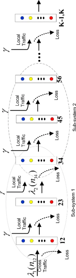
Figure 2.1: A Path in an OBS Network

is linked to OXC 1 by a single fiber and it may be equipped with one or more transmitters. We refer to the traffic generated from the N transmitting end-devices as thecross traffic. In addition, to the cross traffic we consider traffic generated by any other sources in the OBS network. This traffic arrives at the intermediate links of the considered path. We refer to this traffic as thelocal burst traffic. Thelocal traffic is routed toward the same destination end-devices as the cross traffic.

(31)

Figure 2.2: Bursts simultaneously hold wavelengths on multiple links

2.3 The Queueing Network Model

We propose the queueing network model from Figure 2.3 for an OBS path of K links, where the bursts simultaneously hold wavelengths on consecutive links. Since in OBS there is no buffering, in our queueing model there areno queues and burst loss is possible at each node. Each queueing node has W servers, where W is the number of wavelengths per link. Each node in the queueing network does not represent the state of a physical link but rather, as explained below, it represents the number of bursts that occupy wavelengths on a certain number of successive links.

(32)

20

(33)

2. Node (i, i+ 1), 1≤i≤K−1, represents the number of bursts simultaneously holding wavelengths on linki and link (i+ 1). Due to the full wavelength conversion capability at each OBS node, these bursts may occupy one wavelength on linkiand the same or different wavelength on link (i+ 1).

For clarity, in Figure 2.3 we have only shown the queueing network for two different burst sizes: bursts that occupy wavelengths on one link and bursts that occupy wavelengths on two consecutive links. If in the OBS network there were even larger bursts, i.e., bursts that occupy wavelengths on three consecutive links then there would be an additional third row added to the queueing network. In the third row each loss node will model three consecutive links of the OBS path. This idea can be extended to bursts that span any number of links.

(34)

22

Chapter 3

Sub-System Decomposition

Algorithm for Small Number of

Wavelengths

In this chapter, we develop an iterative sub-system decomposition algorithm which solves for the burst loss probabilities in an OBS path with simultaneous possession. This algorithm is recommended for OBS networks where the fibers have a small number of wavelengths because it is based on the numerical solution of Markov Chains. First, in Section 3.1 we look at the case where bursts hold wavelengths on exactly two consecutive links. Then, in Section 3.2 we extend the study to bursts holding wavelengths on one or two number of links as they travel from their source to their destination.

The burst arrival process in this chapter is an m-state Markov process, where

(35)

3.1 Bursts Span Two Links

We begin our study of OBS networks with dynamic simultaneous link possession with the scenario when all bursts are large enough to occupy wavelengths on two links as they propagate through the network. In Figure 2.1, once launched by an end-device, a burst will first occupy a wavelength on link 1 and a wavelength on link 2 simultaneously, then it will move to occupy the same wavelength on link 2 and a wavelength on link 3 simultaneously, and so on until it departs from the network.

This Section is organized as follows. First in 3.1.1 we describe a queueing net-work that models an OBS path with simultaneous link possession, where all bursts hold wavelengths on two consecutive links. We set the the burst arrival process to this queueing network to be a 2-state Markov process, which we refer to as the IDLE-ON arrival pro-cess. Then, in 3.1.2, we propose a sub-system decomposition algorithm that solves for the burst loss probabilities at each link of the OBS path. Further, we illustrate our algorithm through an example in 3.1.3. In 3.1.4 we verify the accuracy of the algorithm and in 3.1.5 we conclude. The material in this Section will appear in [32].

3.1.1 The Queueing Network Model

We propose the queueing network model in Figure 3.1 for an OBS path of K links, where all the bursts simultaneously hold wavelengths on two consecutive links. This queueing network is a subset of the one shown in Figure 2.3. The details of the OBS network under study were described in Section 2.2. Since in OBS there is no buffering, in our queueing model there are no queues and burst loss is possible at each node. The queueing network consists of (K −1) loss nodes linked in tandem. Each node has W

(36)

24

(37)

Figure 3.2: Bursts simultaneously hold wavelengths on two links

queueing notation, the given scenario is described byn12= 2 andn23= 1.

A customer in our queueing network represents a burst, which always occupies a wavelength on two adjacent links at the same time. As the burst propagates through the network, the corresponding customer simply moves from one loss node of the queueing network to the next. Due to the assumption that each OBS node has full wavelength conversion capability, a burst may occupy one wavelength on link (i−1) and the same or different wavelength on link i.

The maximum capacity of each queueing node isW, which means that no more than W burst can be transmitted over the same link at the same time. Therefore the following constraints hold:

ni,i+1≤W, 1≤i≤K−1 (3.1)

whereni (ni,i+1) denotes the number of bursts in queueing nodei(i, i+ 1).

Furthermore, each physical link of the OBS path, with exception of the first and the last, is modeled by two consecutive nodes of the queueing network. For example, link

iis modeled by both node (i−1, i) and node (i, i+ 1). Since link ican transmit no more thanW bursts at one time we also have the following constraints:

ni−₁,i+ni,i+1 ≤W, 2≤i≤K−1 (3.2)

(38)

26

Figure 3.3: Multiplexed IDLE-ON Sources

by the findings in [33] that the blocking probability does not depend on the burst size distribution. We note that in our queueing model it is possible to model the burst length with a Coxian or Phase-Type distribution, but this will increase the dimensionality and thus the complexity of the solution.

(39)

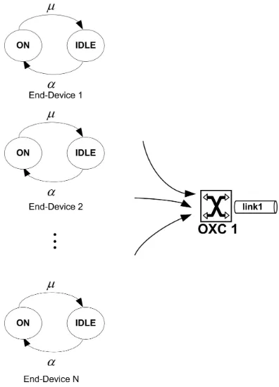
We model each transmitting end-device with the IDLE-ON traffic source, which is the two-state Markov process from Figure 3.3. With the IDLE-ON traffic the burst arrivals are not instantaneous and we can account for the burst transmission time. An OBS end-device is in the ON state when it is transmitting a burst. It remains in this state for the duration of the burst, which is exponentially distributed with a mean of 1/µ. If the end-device is not transmitting a burst then it is in the IDLE state, which is also exponentially distributed with a mean of 1/α. Note, that the IDLE-ON process differs from the popular ON-OFF process, which is used to model the arrival of voice packets. In IDLE-ON, the source transmits only one burst in the ON state and then it moves to the IDLE state. In the ON-OFF model, however, the source continuously transmits packets for the entire time it is in the ON state.

The total traffic due to the N end-devices, referred to from here on as the cross

traffic, is the multiplexed stream of the burst arrivals from all N OBS end-devices. That is, there are N IDLE-ON traffic sources, which generate traffic as shown in Figure 3.3. We assume that all N end-devices are modeled with an identical IDLE-ON source. We note that the case where each of the N end-devices has W transmitters can be modeled by the multiplexed traffic from (N ∗W) traffic sources. We assume that N > W since OBS is designed for backbone networks and the user traffic will be generated by from a large number of sources.

As mentioned previously, each burst occupies two links at once. Therefore, imme-diately upon entering the network, a burst will request wavelengths on links 1 and 2 and if no free wavelengths are available then it will be lost. Also note that only W sources can transmit simultaneously because they all share the wavelengths on links 1 and 2. In our queueing model n12 indicates the number of bursts currently being transmitted over links

1 and 2. That is, n12 sources are in the ON state and the remaining (N −n12) are in the

IDLE state. Burst arrivals are only possible from the traffic sources that are currently in the IDLE state. In view of this, the cross traffic has the following state-dependent arrival rate:

(N −n12)α, 0≤n12≤W (3.3)

(40)

Poisson-28

distributed traffic. This Poisson assumption can be justified by the fact that the OBS technology is mostly likely to be used in a backbone network. To that effect, the local traffic will be generated by a large number of sources and the Palm-Khintchine Theorem [34] says that the superposition of a large number of independent processes behaves asymptotically like a Poisson process. The local traffic arrives at each link, except the first and the last one, and it subsequently becomes part of the cross traffic. That is, a local traffic burst enters the OBS path at an intermediate link and it is routed to the same destination end-devices as the cross traffic. The rate of the Poisson traffic is denoted withγ.

3.1.2 The Solution

The queueing network, described in the previous section, is anopen loss queueing network, which does not have a product form solution. However, this queueing network has the Markovian property because both the duration of the bursts and their interarrival times are exponentially distributed. The underlying Markov process of this queueing network can be completely described by the tuple (n12, n23, ..., nK−₁,K). Depending on the number of links and the number of wavelengths per link, the state space of this Markov process can become quite large. For example, an OBS path of 9 links, where each link’s capacity is 16 wavelengths, will result in a Markov process with 140,930,306 states. For this reason, we analyze the network approximately, by decomposing it into small sub-systems. Each sub-system is a Markov process and we analyze it numerically. In order to analyze each sub-system, we need to obtain probability information from its adjacent sub-systems. This leads to an algorithm where the sub-systems are analyzed iteratively. Below, we describe our algorithm and next we illustrate it through an example.

(41)

the execution time of the algorithm because the total number of sub-systems increased. In either case, when a sub-system has three nodes, the number of states is (see Appendix A):

(W + 1)2+W(2W + 1)(W + 1) 6

which grows in the order ofO(W3).

Yet another possible decomposition is to have two nodes per sub-system withsingle node overlap. If we use use two nodes per sub-system, we can solve OBS paths with much larger number of wavelengths per link than if we use a three node decomposition. The number of states for a sub-system with two nodes is (see Appendix A):

(W + 1)(W + 2) 2

which grows in the order ofO(W2). The accuracy of the two-node decomposition is expected to be lower than that of the three-node decomposition. That is due to the fact that in general the larger the sub-system the better the accuracy of the decomposition algorithm.

In this work, we choose the decomposition of three nodes per sub-system with single node overlap, shown in Figure 3.1. An OBS path ofK links is modeled by a queueing network of (K−1) nodes, which is decomposed into S sub-systems, where:

S=

K−1 2

With this decomposition if the number of nodes in the queueing network is odd then each sub-system will have three nodes. Otherwise, if the number of nodes in the queueing network is even then the last sub-system will contain only two nodes. The analysis of a two-node sub-system is identical to a three-node sub-system. In fact a sub-system with two nodes results in a smaller state space, which is faster to analyze.

The state of a sub-system of three nodes is described by the 3-tuple:

n= (ni−₁,i, ni,i+1, ni+1,i+2)

The state space of a sub-system is subject to the constraints (3.1) and (3.2). We denote the steady-state probability vectors of the sub-systems by πs, 1≤s≤S and obtain them numerically by solving the following linear equations in matrix form:

(42)

30

Event Rate Transition States

cross arrival to (i−₁, i) λs (ni−1,i, ni,i+1, ni+1,i+2)→(ni−1,i+ 1, ni,i+1, ni+1,i+2)

if link i has a free wavelength

no transition if all the wavelengths on link i are busy

local arrival to (i, i+ 1) γ (ni−1,i, ni,i+1, ni+1,i+2)→(ni−1,i, ni,i+1+ 1, ni+1,i+2)

if both links i and i+1 have a free wavelength

no transition if the wavelengths on either link i or link i+1 are all busy

local arrival to (i+1, i+ 2),

γ (ni−1,i, ni,i+1, ni+1,i+2)→(ni−1,i, ni,i+1, ni+1,i+2+ 1)

if both links i+1 and i+2 have a free wavelength

no transition if the wavelengths on either link i+1 or i+2 are all busy

transition from (i−₁, i) to (i, i+ 1)

µni−1,i (ni−1,i, ni,i+1, ni+1,i+2)→(ni−1,i−1, ni,i+1+ 1, ni+1,i+2)

if link i+1 has a free wavelength

no transition if all the wavelengths on link i+1 are busy

transition from (i, i+ 1) to (i+ 1, i+ 2)

µni,i+1 (ni−1,i, ni,i+1, ni+1,i+2)→(ni−1,i, ni,i+1−1, ni+1,i+2+ 1)

if link i+2 has a free wavelength

no transition if all the wavelengths on link i+2 are busy

departure from (i + 1, i+ 2)

µni+1,i+2 (ni−1,i, ni,i+1, ni+1,i+2)→(ni−1,i, ni,i+1, ni+1,i+2−1)

always

Table 3.1: Possible State Transitions for sub-systemswhen in state (ni−₁,i, ni,i+1, ni+1,i+2)

πses=1 (3.5)

where Qs is the transition rate matrix for sub-system s and (3.5) is the normalization condition, es = (1,1, ...,1)T. We solve this system of linear equations using either the forward or backwards Gauss-Seidel method (see Stewart [35]).

3.1.2.1 Rate Matrix Generation

We now show how to construct the state transition matricesQs, 1≤s≤S for the sub-systems. Assume that at time t, sub-systems is in state (ni−₁,i, ni,i+1, ni+1,i+2). Then

at timet+4tit may transition into one of the states shown in Table 3.1. Linkihas a free wavelength if:

(43)

and all of its wavelengths are busy if:

(ni−₁,i+ni,i+1) =W

Note, that in the condition for some of the transitions in Table 3.1 we need to find out whether link (i+2) has a free wavelength. However, the nodes that make up sub-system s can only determine the status of linksiand (i+1). In order to determine the status of link (i+ 2) we need to obtain information from sub-system (s+ 1), which contains all the nodes that model link (i+ 2). So in sub-system (s+1), we useπs+1 and calculate the conditional

probability that link (i+ 2) has a free wavelength given that there are exactly ni+1,i+2 in

node (i+ 1, i+ 2). We denote this probability as:

p(ni+1,i+2) =P rob{link (i+2) has a free wavelength|ni+1,i+2} (3.6)

=P rob{ni+2,i+3 < W−ni+1,i+2|ni+1,i+2}

Note the use of the overlap node (i+ 1, i+ 2) between sub-system s and sub-system (s+1). We make sure that the value of the overlap node is the same in both sub-systems. So in sub-system s we use the probability p(ni+1,i+2) when we need to determine whether a

transition is possible based on the status of link (i+ 2). A burst successfully transitions from node ni,i+1 to node ni+1,i+2 with rate p(ni+1,i+2)ni,i+1µ. Otherwise with a rate of

(1−p(ni+1,i+2))ni,i+1µ, the sub-system transitions to a state where the burst is lost.

3.1.2.2 State-Dependent Arrival Rates

As mentioned previously, the state-dependant arrival process to sub-system 1 is given by the multiplexed IDLE-ON traffic:

λ1(n12) = (N −n12)α, 0≤n12≤W (3.7)

(44)

32

For example, let us consider sub-system s, which consists of nodes (i−1, i), (i, i+1) and (i+ 1, i+ 2). The arrival rate to this sub-system is determined based on sub-system (s−1). Since sub-systems s and (s−1) overlap with node (i−1, i), the arrival rate to sub-systemsis the departure from node (i−2, i−1). In sub-system (s−1), this departure process can be written asµni−₂,i−₁, where 0≤ni−₂,i−₁≤W. However, node (i−2, i−1) is not part of sub-system s and thus we can’t use this description. Instead, we use the overlap node and re-write this departure process to be dependent on ni−1,i. In sub-system (s−1), we calculate the state-dependent arrival rate to sub-system s as follows:

λs(ni−1,i) = W X

j=0

P rob{ni−2,i−1=j|ni−1,i}jµ, 0≤ni−1,i≤W (3.8)

where the probabilities are based onπs−1.

3.1.2.3 The Algorithm

The iterative algorithm to determine the steady-state probabilities vectors for each sub-system is summarized in Algorithm 1. The superscriptmrefers to the iteration number. The algorithm begins with an initialization step, where we ignore all of the link interdepen-dencies between the sub-systems (no conditioning of the transitions, i.e., p = 1) in order to get an initial guess for the steady-state probabilities πs, 1 ≤ s ≤ S. In the iterative step, we solve for πs, 1 ≤ s ≤ S by conditioning some of the transitions in sub-system s based on the probability information from the adjacent sub-systems, i.e., using p(sm). The state-dependent arrival rate for sub-systems is determined based on the current estimate of πs−1. For the last sub-system S, there is no need to condition so we just calculate its

arrival rates fromπS−1 and solve forπS. We repeat the iterative step until the steady-state probabilities converge. The convergence condition is met when:

|π_j(m)−π_j(m−1)| < , 1≤j≤S

whereis a sufficiently small positive number.

3.1.2.4 Calculation of the Burst Loss Probability

(45)

OBS Path of K links is modeled by a queueing network of (K−1) nodes. The queueing network is decomposed intoS sub-systems;

Initialization Step;

forj= 1 :S do

//Calculate the state-dependent arrival rates;

if j= 1 then

forλ1 use (3.7); else

forλ(1)_j use (3.8), based onπ_j(1)−1 ; end

//Ignore the link interdependencies between the adjacent;

//sub-systems by setting p=1; generate Q(1)_j ;

solve forπ(1)_j ;

end

Iterative Step m;

form= 2 until convergence do forj= 1 :S do

if j6= 1 then

calculate λ(_jm) by using (3.8) based on π_j(m−1) ; end

if j6=S then

//Calculate the link interdependencies between two adjacent;

//sub-subsystems;

calculate p(_jm) based onπ_j(m₊₁−1) by using (3.6) ;

else

//for the last sub-system there are no link dependencies;

p(_Sm) = 1

end

generate Q(_jm) by using p(_jm) ; solve for π_j(m) ;

end end

(46)

34

probability that a burst is lost upon moving from links (i−2) and (i−1) to links (i−1) and iwith bi−1,i. Note, that this burst already has a wavelength on link (i−1) and it is blocked because link idoes not have any free wavelengths.

Since we model the arrival rates to be state-dependent, the burst loss probabilities are obtained based on the steady-state vectors πs, 0 ≤ s ≤ S in combination with the appropriate arrival rates. In Section 3.1.2.2 we have already obtained the state-dependant arrival rates to all of the overlap nodes. Therefore the burst loss probability at the first overlap node of sub-system s is the following conditional probability:

bi−1,1=P rob{link i is full|arrival to node (i−1, i)} (3.9)

= W X

j=0

P rob{ni,i+1=W −j|ni−1,i =j}λs(j)

W X

j=0

P rob{ni−1,i=j}λs(j)

where all the probabilities are obtained using the steady state probability vector πs. The numerator represents the portion of bursts that arrive at node (i−1, i) and find all of the wavelengths on link i to be busy. The form of the numerator is justified by the fact that

λs is a state-dependant arrival rate. The denominator represents the average burst arrival rate to node (i−1, i).

We haven’t yet calculated the arrival rate for nodes that are not overlap nodes, i.e., the middle nodes of the sub-systems. For these nodes, we use the departure process from the previous node and thus the burst loss probability is:

bi−1,i=P rob{link i is full|departure from node (i−2, i−1)} (3.10)

= W X

j=0

P rob{ni−1,i+ni,i+1 =W |ni−2,i−1=j}jµ

W X

j=0

P rob{ni−2,i−1 =j}jµ

(47)

Figure 3.4: Queueing Network for an OBS path of 6 links with 2 wavelengths per link

on link i to be busy. The denominator represents the average departure rate from node (i−2, i−1).

3.1.3 Example

In this section, we illustrate our algorithm through an example. We consider an OBS path, consisting of 6 links connected in tandem. Each link has two wavelengths, i.e.,

W = 2. This OBS path is modeled by the five-node queueing network, shown in Figure 3.4. The queueing network is decomposed into two sub-systems each containing three nodes. Sub-system 1 consists of nodes 12, 23 and 34 while sub-system 2 consists of nodes 34, 45 and 56. We note that the two sub-systems overlap with node 34.

The traffic load λ1(n12) to the OBS path is generated by N OBS users, modeled

by the multiplexed IDLE-ON process described in Section 3.1.1. Therefore, the cross arrival rate to link 1 is λ1(n12) = (N −n12)α, 0≤ n12 ≤2. The Poisson-distributed local traffic

has an average rate γ.

Analysis of Sub-system 1

The state of sub-system 1 is described by the 3-tuple vector:

n= (n12, n23, n34) (3.11)

The state space is subject to the constraints (3.1) and (3.2) and it consists of the following states:

(48)

36

Using the transitions from Table 3.1 we construct the rate matrix Q1 for

sub-system 1:

Q1= 2 6 6 6 6 6 6 6 6 6 6 6 6 6 6 6 6 6 6 6 6 6 6 6 6 6 6 6 6 6 6 6 4

? γ 0 γ 0 0 λ1(0) 0 0 0 0 0 0 0

µ ? γ 0 γ 0 0 λ1(0) 0 0 0 0 0 0

0 2µ ? 0 0 0 0 0 λ1(0) 0 0 0 0 0

µq µp 0 ? γ γ 0 0 0 λ1(0) 0 0 0 0

0 µq µp µ ? 0 0 0 0 0 λ1(0) 0 0 0

0 0 0 2µq 2µp ? 0 0 0 0 0 0 0 0

0 0 0 µ 0 0 ? γ 0 γ 0 λ1(1) 0 0

0 0 0 0 µ 0 µ ? γ 0 γ 0 λ1(1) 0

0 0 µ 0 0 0 0 2µ ? 0 0 0 0 λ1(1)

0 0 0 0 0 µ µq µp 0 ? γ 0 0 0

0 0 0 0 µ 0 0 µq µp µ ? 0 0 0

0 0 0 0 0 0 0 0 0 2µ 0 ? γ 0

0 0 0 0 0 0 0 0 0 0 2µ µ ? γ

0 0 0 0 0 0 0 0 2µ 0 0 0 2µ ?

3 7 7 7 7 7 7 7 7 7 7 7 7 7 7 7 7 7 7 7 7 7 7 7 7 7 7 7 7 7 7 7 5 (3.12)

where each diagonal element, indicated by ?, is the negative sum of all the non-zero tran-sition rates on the same row.

In sub-system 1, the number of bursts at links 1, 2 or 3 can be easily calculated. The number of bursts at link 1 is simply n12. The number of bursts at link 2 is computed

by adding up the number of bursts at nodes 12 and 23. The number of bursts occupying a wavelength on link 3 is computed by adding the number of bursts at nodes 23 and 34.

However, for some of the transitions we need to determine the status of link 4. For example, a burst transition from node 23 to node 34 is only possible if link 4 has a free wavelength. However, sub-system 1 doesn’t contain all the queueing nodes that model link 4. We address this problem by conditioning these transitions in sub-system 1 using probability information from sub-system 2. Suppose that a burst is about to depart links 2 and 3 and move into links 3 and 4 and the state of sub-system 1 is currently (1,1,1). There are two possibilities for that burst: it could move on successfully or it could be dropped. If the burst is successfully transmitted then the sub-system will move into state (1,0,2) and if it is lost it will move into state (1,0,1). The transition rate out of the current state is computed using probability information from sub-system 2. We find the conditional probability that link 4 has a free wavelength given that there are n34 bursts

(49)

1 and 2 and thus it must have the same value in both sub-systems. Therefore, in sub-system 2 we find the conditional probability that a burst successfully transitions from links 2 and 3 to links 3 and 4:

p(n34) =P rob{link 4 has a free wavelength|n34} (3.13)

=P rob{n45< W−n34|n34}

The rate of successful burst transition becomes µp. The loss transition rate is µq, where

q = 1−p. These are the values for p and q used in Q1. Once we have constructed Q1 we

use (3.4) and (3.5) to solve forπ1.

Analysis of Sub-systems 2

The arrival process to sub-system 2 consists of the cross traffic, which departs from links 2 and 3 and attempts to enter links 3 and 4 in addition to the Poisson-distributed local trafficγ at link 3. The departure process from links 2 and 3 is determine based on the steady-state probability vector of sub-system 1:

λ2(n34) =

W X

j=0

P rob{n23=j|n34}jµ, 0≤n34≤W (3.14)

With the addition of the local traffic, the total arrival rate to sub-system 2 becomes

λtot

2 (n34) =λ2(n34) +γ (3.15)

We analyze sub-system 2 following the same procedure as for sub-system 1. We use the transitions from Table 3.1 and generate the rate matrixQ2. This requires the status

(50)

38

Q2= 2 6 6 6 6 6 6 6 6 6 6 6 6 6 6 6 6 6 6 6 6 6 6 6 6 6 6 6 6 6 6 6 4

? γ 0 γ 0 0 λtot

2 (0) 0 0 0 0 0 0 0

µ ? γ 0 γ 0 0 λtot

2 (0) 0 0 0 0 0 0 0 2µ ? 0 0 0 0 0 λtot

2 (0) 0 0 0 0 0

µ µ 0 ? γ γ 0 0 0 λtot

2 (0) 0 0 0 0

0 µ µ µ ? 0 0 0 0 0 λtot

2 (0) 0 0 0

0 0 0 2µ 2µ ? 0 0 0 0 0 0 0 0

0 0 0 µ 0 0 ? γ 0 γ 0 λtot

2 (1) 0 0

0 0 0 0 µ 0 µ ? γ 0 γ 0 λtot

2 (1) 0

0 0 µ 0 0 0 0 2µ ? 0 0 0 0 λtot

2 (1)

0 0 0 0 0 µ µ µ 0 ? γ 0 0 0

0 0 0 0 µ 0 0 µ µ µ ? 0 0 0

0 0 0 0 0 0 0 0 0 2µ 0 ? γ 0

0 0 0 0 0 0 0 0 0 0 2µ µ ? γ

0 0 0 0 0 0 0 0 2µ 0 0 0 2µ ?

3 7 7 7 7 7 7 7 7 7 7 7 7 7 7 7 7 7 7 7 7 7 7 7 7 7 7 7 7 7 7 7 5 (3.16)

where each diagonal element, indicated by?, is the negative sum of the all the other non-zero elements on the same row. OnceQ2 is generated, we use (3.4) and (3.5) to findπ2.

The Iterative Algorithm

The algorithm begins with an initial guess for the steady-state probability vectors of the two sub-systems by settingp= 1 andq= 1−p= 0. In the iterative step, we solve for a new π1, using p calculated based on the current known value forπ2. Then, we calculate

a new state-dependent arrival rateλ2 to sub-system 2 and solve for a new value for π2. We

repeat these steps iteratively untilπ1 and π2 converge.

Burst Loss Probability

We now show how to use the steady-state vectors of the sub-systems to calculate the burst loss probabilities at each link of the OBS path.

Burst Loss Probability b2 at node 12:

The burst loss probability of the cross traffic at link 2 is given by the expression:

b2=P rob{Link2is f ull|Arrival to node12}

=

PW

i=0P rob{n23=W −i|n12=i}(N −i)α

PW

i=0P rob{n12=i}(N −i)α

(51)

where all the probabilities are obtained from π1 Burst Loss Probability b3 at middle node 23:

The burst loss probability of the cross traffic at link 3 is given by:

b3 =P rob{Link3is f ull|Departure f rom node12}

=

PW

i=0P rob{n23+n34=W | n12=i}iµ

PW

i=0P rob{n12=i}iµ

(3.18)

All the probabilities in the above expression come fromπ1. Burst Loss Probability b4 at node 34:

The cross traffic burst loss probability at link 4 is given by:

b4 =P rob{Link4is f ull|Arrival to node 34}

=

PW

i=0P rob{n45=W −i|n34=i}λ2(i)

PW

i=0P rob{n34=i}λ2(i)

(3.19)

where, the probabilities come from π2 and λ2(i) is the state-dependent cross traffic arrival

rate to sub-system 2.

Burst Loss Probability b5 at node 45:

The burst loss probability at link 5 is calculated the exact same way as for link 3 but all the information comes fromπ2.

3.1.4 Numerical Results

We now present numerical results for the cross traffic burst loss probability at each link of an OBS path by utilizing our decomposition algorithm and we compare them to simulation results. The analytical results are obtained using Matlab code, while the sim-ulation results are obtained with a custom event-driven C++ simulator. For each reported statistic, we ran the simulation 30 times for a sufficiently long time in order to compute the 95% confidence intervals. Note, that the simulation results are plotted along with their confidence intervals but the confidence intervals are quite small and hardly visible on the plots. We only present a few specific examples but we tested our algorithm for a variety of input parameters and we found it to have good accuracy.

(52)

40

0 0.1 0.2 0.3

2 3 4 5 6 7

Link

α=1.0

α=0.8

α=0.6

α=0.4

α=0.2

Sim, α=0.2 Num, α=0.2 Sim, α=0.4 Num, α=0.4 Sim, α=0.6 Num, α=0.6 Sim, α=0.8 Num, α=0.8 Sim, α=1.0 Num, α=1.0

Figure 3.5: Burst Loss Probability for W=16, L=8, N=32, low to high load

0.1 0.2 0.3 0.4 0.5 0.6 0.7 0.8

2 3 4 5 6 7

Utilization

Link

(53)

0 0.05 0.1 0.15

2 3 4 5

Link

Figure 3.7: Burst Loss Probability for W=8, L=6, N=16, low to moderate load

0.05 0.1 0.15 0.2 0.25 0.3 0.35 0.4 0.45

2 3 4 5

Utilization

Link

(54)

42

3 4 5

0 1 2 3 4 5 6 7 8 9 10 11 12 13 14 15 16

Arrival Rate

n₁₂ Sub-System 1

Sim, λ₁(n₁₂) Num, λ1(n12)

0 1 2 3 4

0 1 2 3 4 5 6 7 8 9 10 11 12 13 14 15 16

Arrival Rate

n₃₄ Sub-System 2

Sim, λ2(n34)

Num , λ₂(n₃₄)

0 1 2 3 4

0 1 2 3 4 5 6 7 8 9 10 11 12 13 14 15 16

Arrival Rate

n₅₆ Sub-System 3

Sim, λ₃(n₅₆) Num, λ₃(n₅₆)

(55)

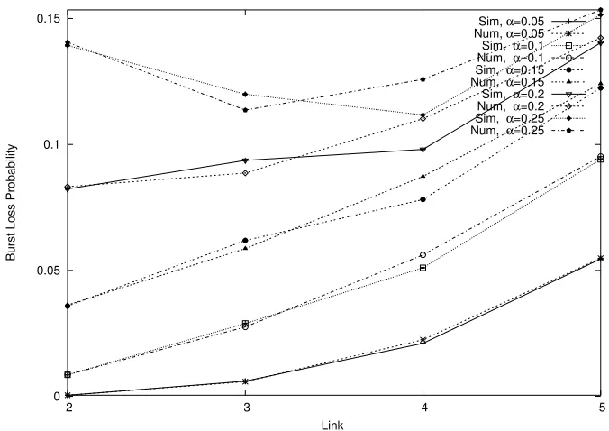
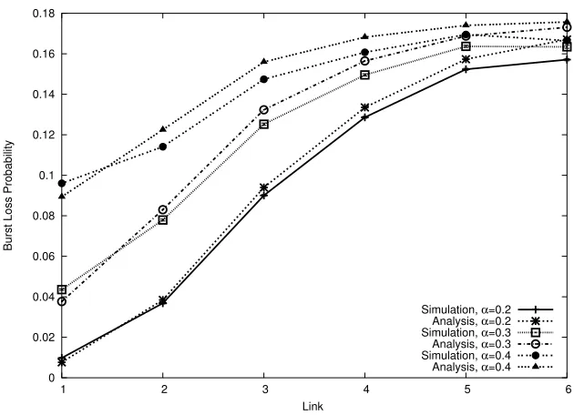
there are N = 32 OBS transmitting end-devices, each modeled by an IDLE-ON source. The intensity of the cross traffic is varied based on the time spent in the IDLE state, i.e., based on the value of α. The local arrivals are Poisson-distributed and their average rate is the same at each link of the OBS path, i.e.,γ = 0.5. The analytical results are obtained by decomposing the queueing network into 3 sub-systems each containing 3 nodes and overlapping by a single node.

In Figure 3.5, we plot the burst loss probabilitybi at each link i, wherei= 2,3...,7 for various values ofα. The plot shows that our analytical results match quite closely the results obtained through simulation. There is a slightly higher error at links 4 and 6, whose burst loss probabilities are calculated at the overlap nodes between the three sub-systems. The slightly higher error is due to the approximation used in calculating the state-dependent arrivals.

We observe afiltering effect of the burst loss probabilities. That is, as we increase the load at the front of the OBS path, the burst loss probability at link 2 rapidly increases but that phenomenon does not carry over to the other links in the path. Each link acts as a filter because it drops some of its incoming bursts and thus the load to the following link is reduced. In addition, there is a tendency for the burst loss probability to slightly increase from link 2 to link 7, which is caused by local arrivals at each link. The reason is that any local traffic burst, that is not lost at the link where it arrives, is carried on as part of the cross traffic to the following link. We do not plot the cross traffic burst loss at links 1 and 8 because it is zero.

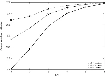
For this scenario, we also plot the utilization λ/(µW) of each link in Figure 3.6. We observe that at the lower load the link utilization increases from link 2 to link 7 because of the added local arrivals. However, as we increase the load, the utilization of links 5, 6 and 7 converges. Once again, that is explained by the previously noted filtering effect. It is also interesting to note that at utilization of 50% and below, the burst loss probability is around 0.1.

In Figure 3.7 we plot the burst loss probabilities for an OBS path withL= 6 links and W = 8 wavelengths but this time the load is low to moderate. Again, the accuracy of our algorithm is very good with the largest error at link 4, which is the overlap node in the analytical solution. The utilization of this scenario is plotted in Figure 3.8. Note again, that at utilization below 50%, the burst loss probability is kept below 0.15.