ABSTRACT
SEDHAI, SUMIT RAJ. A Multiscale Flame-Embedding Framework for Turbulent Combustion using LES-ODT. (Under the direction of Dr. Tarek Echekki.)
A novel method for the simulation of a turbulent non-premixed flame is formulated. The
simulation strategy is a multi-scale framework with a flame-embedding approach consisting
of a coupling between a large-eddy simulation (LES) and a one-dimensional turbulence model
(ODT). The coarse grid LES model simulates large scale flow phenomena. High resolution ODT
grids embedded in the LES grid solve for fine-grained effects of combustion including chemistry
and species transport. The ODT solution is used as a closure for LES governing equations.
A Lagrangian approach is used for embedding the ODT domains in which they are attached
to the flame and advected along with the flow. High resolution ODT grids exist only around the
flame surface, where the important combustion processes occur. As the grid resolution is low
in locations without flame, computation cost is relatively low while maintaining high fidelity
of solution. Flame surface is defined from mixture fraction field in LES, corresponding to the
stiochiometric mixture fraction value. FDS, an open source code, is used as an LES solver.
Information is passed between the LES and ODT grids by the processes of interpolation and
filtering. Some strategies for filtering data from fine grained ODT grid to coarse LES grid have
been studied.
The ability of the model to capture important fine-grained effects, such as finite-rate
chem-istry effects and flame extinction, is demonstrated. The model can be extended to include more
c
Copyright 2011 by Sumit Raj Sedhai
A Multiscale Flame-Embedding Framework for Turbulent Combustion
using LES-ODT
by
Sumit Raj Sedhai
A thesis submitted to the Graduate Faculty of North Carolina State University
in partial fulfillment of the requirements for the Degree of
Master of Science
Mechanical Engineering
Raleigh, North Carolina
2011
APPROVED BY:
Dr. Alexei Saveliev Dr. Thomas Ward
Dr. John Harlim Dr. Tarek Echekki
DEDICATION
BIOGRAPHY
The author was born in Kathmandu, Nepal. He completed his Bachelor’s degree in
Mechan-ical Engineering from Tribhuvan University, Pulchowk Campus. After that, he joined North
ACKNOWLEDGEMENTS
I would like to extend my sincere gratitude to my advisor Dr. Tarek Echekki, without whose
support this thesis would not have been possible. I shall always be indebted to him for his
brilliant mentorship, encouragement and inspiration.
I would also like to thank Dr. Alexei Saveliev, Dr. Thomas Ward and Dr. John Harlim for
agreeing to serve on my committee. Their guidance and valuable insights have been of much
importance in the completion of this work.
I would like to thank Sivaramakrishnan Balasubramanian for providing me his code and his
valuable guidance towards the beginning of my study. I am also indebted to the generosity of
Dr. Elisabeth Larsson and Dr. Bengt Fornberg who provided me with their RBF codes.
Finally, I would like to express my appreciation to friends and family for their motivation
and love. My family, for their unwavering support, and for the regular phone calls that would
put the calendar to shame. My labmates, for making it such an enjoyable workplace, and for
their support during times of need – like homework, among others. My roommate, for doing
my part of the chores without complaint when I would turn up late. My friends, for keeping
TABLE OF CONTENTS
List of Tables . . . vii
List of Figures . . . .viii
Chapter 1 Introduction . . . 1
1.1 Background . . . 1
1.2 Existing Methods in Combustion Simulation . . . 2
1.2.1 Direct Numerical Simulation . . . 2
1.2.2 Reynolds-Averaged Navier-Stokes . . . 3
1.2.3 Large-Eddy Simulation . . . 3
1.2.4 Closure Strategies in LES . . . 3
1.3 Motivation . . . 4
1.4 Objective . . . 5
1.5 Outline . . . 6
Chapter 2 Large-Eddy Simulation . . . 7
2.1 Objective . . . 7
2.2 Introduction . . . 7
2.3 Governing Equations . . . 8
2.4 Fire Dynamics Simulator (FDS) Model . . . 11
2.4.1 Model Features . . . 11
2.4.2 The Subgrid-scale Model . . . 12
2.4.3 Mixture Fraction Based Combustion Model . . . 13
2.4.4 The Flame Surface and the Marching Cubes Algorithm . . . 16
Chapter 3 The One-Dimensional Turbulence Model . . . 17
3.1 Objective . . . 17
3.2 Introduction . . . 17
3.3 ODT Governing Equations . . . 18
3.4 Turbulence Modeling . . . 19
3.4.1 Eddy Size Determination . . . 21
3.4.2 Eddy Location Determination . . . 21
3.4.3 Eddy Rate Distribution . . . 22
3.4.4 ODT Acceptance Probability . . . 22
3.4.5 The Triplet Map . . . 22
3.4.6 The Pressure-Scrambling Model . . . 24
3.5 Computation of Scalars . . . 25
3.5.1 Viscosity . . . 25
3.5.2 Mass Diffusivity . . . 26
3.5.3 Thermal Conductivity . . . 26
3.5.5 The Chemical Reaction Rate . . . 27
Chapter 4 LES-ODT Coupling . . . 29
4.1 Objective . . . 29
4.2 LES-ODT Coupling – Lagrangian Formulation . . . 29
4.3 LES-ODT Information Exchange . . . 31
4.4 Interpolation . . . 31
4.5 Initialization of Scalar Parameters . . . 34
4.6 Management of ODT Domains . . . 35
4.6.1 Flame Displacement Speed . . . 35
4.7 Filtering . . . 36
4.7.1 Region of Influence of Domains . . . 37
4.7.2 Method of Cubature . . . 39
4.7.3 Implementation . . . 39
Chapter 5 Simulation Condition and Results . . . 41
5.1 Overview . . . 41
5.2 Simulation Condition . . . 42
5.3 ODT Solutions of Scalar Parameters . . . 44
5.4 Finite-Rate Chemistry Effects . . . 46
5.5 Addition and Redistribution of ODT Elements . . . 46
5.6 Filtering Process . . . 49
5.7 Filtering using RBF . . . 51
5.7.1 Error analysis . . . 52
5.8 Simulation Time . . . 54
5.9 Simulated Flame . . . 54
Chapter 6 Conclusions and Future Work . . . 59
6.1 Conclusions . . . 59
6.2 Recommendations for Future Work . . . 60
References. . . 61
Appendix . . . 64
Appendix A Radial Basis Functions . . . 65
A.1 Introduction . . . 65
A.2 Mathematical Representation . . . 66
A.3 Basic Functions . . . 68
LIST OF TABLES
Table 3.1 Constants used in the calculation of ΩD . . . 26
LIST OF FIGURES
Figure 1.1 Schematic of LES-ODT coupling using Eulerian approach [4]. ODT
ele-ments in only one direction have been shown. . . 4
Figure 2.1 Oxygen-temperature phase space showing where combustion is allowed to take place [23] . . . 15
Figure 3.1 Flowchart for a stirring process in ODT. . . 20
Figure 3.2 Effect of the triplet map on a scalar field. . . 23
Figure 4.1 Embedding strategy: The ODT domains attached to the flame brush. The orientation of domains is normal to the flame surface. . . 30
Figure 4.2 Embedding strategy: ODT domains in an LES grid . . . 31
Figure 4.3 Exchange of information between LES and ODT . . . 32
Figure 4.4 Trilinear interpolation on an ODT grid point . . . 33
Figure 4.5 State relation: Initialization of ODT scalars from the mixture fraction. . 34
Figure 4.6 Anchoring and transport of ODT domains. . . 36
Figure 4.7 Kernel function used in the filtering process as a function of distance. . . 37
Figure 4.8 Averaging the data on an ODT domain. . . 38
Figure 4.9 Region of influence of an ODT domain. . . 38
Figure 5.1 Computational domain used in the simulation. . . 42
Figure 5.2 Temperature on an ODT domain. . . 44
Figure 5.3 Fuel mass fraction on an ODT domain. . . 45
Figure 5.4 Oxidizer mass fraction on an ODT domain. . . 45
Figure 5.5 Effect of turbulence and finite-rate chemistry on temperature. . . 46
Figure 5.6 Unveven distribution of ODT elements when not corrected. . . 47
Figure 5.7 ODT elements leaving the flame surface from the flame tip. . . 48
Figure 5.8 ODT elements attached to the flame surface (in half-section). . . 48
Figure 5.9 Filtered density and FDS density in x-plane. . . 50
Figure 5.10 Filtered density and FDS density in y-plane. . . 50
Figure 5.11 Grid cells with filtered values. . . 50
Figure 5.12 Randomly distributed data points used as a test grid. . . 52
Figure 5.13 Track-data points used as a test grid. . . 53
Figure 5.14 Error as a function ofεfor randomly distributed points. . . 53
Figure 5.15 Error as a function ofεfor track-data points. . . 54
Figure 5.16 Simulation time for LES and LES-ODT model. . . 55
Figure 5.17 Temperature plot at 0.10 s. . . 55
Figure 5.18 Temperature plot at 0.20 s. . . 56
Figure 5.19 Temperature plot at 0.25 s. . . 57
Figure 5.20 Simulated flame 0.10 s. . . 57
Figure 5.22 Simulated flame at 0.25 s. . . 58
Chapter 1
Introduction
1.1
Background
The importance of the phenomenon of combustion in engineering requires no explanation.
Combustion is encountered in a variety of applications around us, such as internal combustion
engines, jet engines, furnaces and boilers. To develop the ability to understand this phenomenon
and to predict its processes has been, and continues to be, of particular interest to scientists
and engineers. For hundreds of years scientists have studied combustion; nevertheless, due to
its complex nature, newer developments in this field continue to occur. Traditionally, scientific
studies on this subject have been made using theoretical and experimental methods. More
recently, after the advent of modern computers, computational methods have become popular.
Several numerical methods for simulating combustion processes have been developed as more
research in this field continues. The goal of developing new methods is to improve the accuracy
while reducing the cost of computation. This study is one such attempt in formulating a
novel approach for simulating a combustion process, in particular a turbulent non-premixed
flame. The method discussed involves the coupling of a 1-D model known as One Dimensional
1.2
Existing Methods in Combustion Simulation
A combustion process occurs as a result of chemical reaction between a fuel and an oxidizer.
Heat is produced during the process and it is accompanied by transport of molecules. Hence,
it entails the processes of fluid dynamics, thermodynamics and chemistry. A wide range of
scales in both space and time is involved. This includes small scales of chemical reaction as well
as relatively large scales of fluid mechanics. This makes computation of combustion processes
particularly challenging. Computational approaches for reacting flows can be divided into three
categories based on the resolved scales in the flow [26].
1. Direct Numerical Simulation (DNS)
2. Reynolds-Averaged Navier-Stokes (RANS)
3. Large-Eddy Simulation (LES)
1.2.1 Direct Numerical Simulation
In Direct Numerical Simulation (DNS), all temporal and scalar scales are resolved and the
transport equations are directly solved. The grid resolution is very fine (of the order of
mi-crons), and the governing equations are directly solved. As the grid resolution is fine, the time
steps taken are also extremely small. The main advantage of DNS is that the information it
provides regarding the flow field is the most accurate of all available methods and parallels
experimentation. Measurements that can be difficult through experimentation can be made
using DNS and it is also used in validating other methods. However, due to its resolution the
computational costs are high. This cost increases rapidly with physical size and complexity of
chemical reaction. This method is practical only in cases of small domain sizes and relatively
1.2.2 Reynolds-Averaged Navier-Stokes
Reynolds-Averaged Navier-Stokes (RANS) is an averaging method and the cheapest among
the three. The mean values of scalars and momentum are obtained by solving the averaged
governing equations for scalars and momentum. The averaging can be both temporal and
spatial. The averaging results in the loss of unresolved details, and some method for closure
of these terms is required. Besides being the cheapest it is also the least accurate of the three
methods.
1.2.3 Large-Eddy Simulation
Large-Eddy Simulation (LES) lies between DNS and RANS both in terms of cost and
accu-racy. This method was proposed by Smagorinsky [34] and further explored by Deardorff [7] for
turbulent non-reacting flows. In LES, the effect of the large scales is directly computed, and
only the small subgrid scales are modeled [14]. LES is based on the idea that the large and
small scale turbulent processes can be decoupled. While the flow field is mainly defined by the
larger scale eddies, the smaller scale ones are universal and isotropic throughout the flow. The
grid size is coarse and is so chosen such that only the large scales processes are resolved. This
is essentially a low pass filtering of the governing equations. The filtered governing equations
thus have unclosed terms and other methods are used for closure. Since ours is an LES model,
we briefly introduce some of the closure strategies commonly used in LES.
1.2.4 Closure Strategies in LES
The filtered equations in both LES and RANS give rise to unclosed terms which are often
non-linear. Several strategies have been used to resolve these terms, the oldest of them being the
Eddy Dissipation Concept (EDC) and the Eddy Break-Up (EBU) model. More sophisticated
approaches include the Flamelet model, Conditional Model Closure (CMC) model, and the
transported Filtered Density Function (FDF) model [4]. More recent developments are the
are low dimensional models and are based on a one-dimensional physical domain. They treat
molecular reaction-diffusion and turbulent stirring by distinct processes, and the scalars in
consideration are resolved both spatially and temporally. Because they are low-dimensional
models, high resolution can be obtained with much less computational complexity. The ODT
model will be further discussed in subsequent chapters.
1.3
Motivation
Large-Eddy Simulation (LES) is emerging as a preferred method in combustion simulation.
This is due to its ability to deliver good results at a relatively low cost. As discussed earlier,
a separation of scales is implicit in LES, the larger scales being resolved and the smaller scales
being modeled. Thus, if LES is used in conjunction with a robust sub-grid scale model high
fidelity predictions can be achieved. The ODT is one such sub-grid scale model.
The coupling of LES and ODT has been previously done by Cao and Echekki [5]. In this
study, a novel method consisting of embedding fine 1D ODT grids in a course 3D LES grid is
developed and the model validated. The grid embedding is done using an Eulerian approach,
i.e. the ODT grids are stationary in space. The ODT grids are to be embedded throughout
the domain of simulation as shown in Figure 1.1.
The disadvantage of the Eulerian approach is that the high resolution ODT grids cover the
entire domain and hence increase the computational cost. The physical size of the simulated
flame is limited due to this constraint. In flames, high resolution is desired mainly around
the flame since that is where the small scale chemistry effects reside. This is addressed in the
current study by adopting a Lagrangian approach, where the ODT domains are attached to
the flame surface and move with the flow. It is demonstrated that flames of considerable sizes
can be simulated with this method at a relatively modest cost. A preliminary study on the
Lagrangian approach of LES-ODT coupling was done by Balasubramanian [2], in which a fixed
number of ODT domains were used. In the present study, the number of ODT domains depends
on the flame size and domain management is introduced. A number of methods for filtering
have been investigated.
The LES code used in this study is the Fire Dynamics Simulator (FDS), an open source
code developed by National Institute of Standards and Technology (NIST).
1.4
Objective
The objective of this study is to develop and implement an LES-ODT coupled modeling
frame-work with a Lagrangian approach for a non-premixed flame. The LES solutions are carried out
in three dimensions and the ODT solutions are in 1D. The 1D domains containing the ODT
solutions are attached to the flame brush defined in the 3D domain through a flame surface
marker and carried along with the flame as it evolves. There is exchange of information
be-tween LES and ODT solutions such that the ODT model provides closure to the LES governing
equations. This is essentially a flame-embedding approach in which high resolution 1D ODT
grids are attached to a flame. The ODT grids capture small scale effects and provide closure
1.5
Outline
This section describes the organization of the rest of the thesis.
• Chapter 2 gives an introduction to the LES method.
• Chapter 3 gives an introduction to the ODT model used.
• Chapter 4 describes the method of LES and ODT coupling.
• Chapter 5 describes the simulation conditions and presents the results.
Chapter 2
Large-Eddy Simulation
2.1
Objective
In this chapter, the formulation and numerical implementation of the large-eddy simulation
(LES) model is described. The theory behind LES and its governing equations are discussed.
In the later part of the chapter the working of Fire Dynamics Simulator (FDS), the source code
for LES solver, is discussed.
2.2
Introduction
Large-eddy simulation is a Computational Fluid Dynamics (CFD) model for turbulence
simula-tion. In LES, the larger three-dimensional turbulent motions are directly represented, whereas
the effects of the smaller scale motions are modeled [28]. LES can be implemented in a grid
much coarser than direct numerical simulation (DNS) and hence has a much lower computaional
cost. Compared to Reynolds-averaged Navier-Stokes (RANS), it has better fidelity but it is more
expensive.
LES is based on the concept that much of the energy in a turbulent flow resides in the large
scale eddies and the flow characteristics are defined by them. The smaller eddy statistics are
In principle, LES is a low-pass filtering process applied to the Navier-Stokes equations.
In combustion modeling, however, LES alone is not suitable since important effects such as
chemical reaction and species transport occur at the small (subgrid) scales.
Filtering The filter in LES can be either implicit or explicit. In the former case the filter
is implicitly defined by the grid used, while in the latter explicit mathematical filtering
func-tions are defined. The implicit filter is more commonly used as it is computationally efficient.
Mathematically, a filtered quantity is defined as:
u(x) = Z
G(r)u(x−r)dr (2.1)
where integration is over the entire flow domain, and the specified filter functionG(r) satisfies
the normalization condition
Z
G(r)dr= 1 (2.2)
Commonly used filter functions are the box filter, the Gaussian filter and the sharp spectral
filter [28]. The velocity field is thus decomposed as:
u(x) =u(x) +u0(x) (2.3)
whereu0(x) is the unresolved or residual field.
2.3
Governing Equations
The LES governing equations are obtained by performing filtering operations on the general
transport equations. These are given below [1] [24]. In the following equations, ρ, u, p and h
space and time coordinates.
Conservation of Mass
∂ρ¯
∂t + ∂ρ¯u˜i
∂xi
= 0 (2.4)
Conservation of Momentum
∂
∂t( ¯ρu˜i) =− ∂p¯
∂xi − ∂
∂xj
( ¯ρu˜iu˜j) +
∂¯τij
∂xj
+ ¯ρfi+
∂ ∂xj
τijSGS (2.5)
where the stress tensor τij is
τij =µ
∂ui
∂xj +∂uj
∂xi
− 2 3δij
∂uk
∂xk
(2.6)
δij is the Kronecker delta defined as
δij =
0 if i6= j
1 if i = j
and τijSGS is the subgrid stress tensor given by
τijSGS = ¯ρu˜iu˜j−ρ¯ugiuj (2.7)
Conservation of Energy
∂
∂t( ¯ρ˜h) = Dp¯
Dt + ¯˙q
000−q¯˙000
b −
∂q¯˙i00 ∂xi
+ ∂
∂xi
( ¯ρ˜hu˜i−ρ¯ghui) + ¯ε (2.8)
whereεis known as thedissipation rate. It is the rate at which kinetic energy is transferred to
ε≡τij
∂ui
∂xj =µ
"
2SijSij − 2 3 ∂uk ∂xk 2# (2.9)
Sij is the symmetric strain tensor given as
Sij = 1 2
∂ui
∂xj +∂uj
∂xi
(2.10)
The bar symbol ( ¯·) is the filter operator as defined above. The symbol tilde ( ˜·) is the density weighted average known as Favre average. It is defined as:
˜ Φ = ρΦ
¯
ρ (2.11)
In Eq. 2.8, ¯˙q000 is the heat release rate per unit volume from a chemical reaction. The term ¯˙qb000
is the energy transferred to the evaporating droplets. The term ¯˙qi00 represents the conductive and radiative heat fluxes[23].
¯˙
qi00=−k∂T ∂xi
+X
α
hαρDα
∂Yα
∂xi
+ ¯˙qr,i00 (2.12)
wherek is the thermal conductivity,Dα is the diffusivity of species α, and ¯˙q00r,i is the radiative heat flux.
The numerical algorithm of the LES solver makes a low Mach number assumption and
combines the mass and energy equations through divergence.
Ideal Gas Equation
¯
p= ρRT¯
W (2.13)
2.4
Fire Dynamics Simulator (FDS) Model
FDS is a Computational Fluid Dynamics (CFD) model of fire-driven fluid flow. It solves
numericallly an LES form of the Navier-Stokes equations appropriate for low-speed, thermally
driven flow with an emphasis on smoke and heat transport from fires [23]. It also has a DNS
option.
It is an open source code written in FORTRAN 90 and developed by the National Institute
of Standards and Technology (NIST) in cooperation with VTT Technical Research Centre of
Finland. It is primarily aimed at simulating building fires, fire spread and fire growth. The
first version of FDS was released in February 2000, and since then it has gone through many
upgrades. FDS v5 is the latest version and is the one used in this study. It is widely used in
fire simulation and various add-ons to it have been developed. FDS along with Smokeview [12],
a companion program for visualizing the results, is provided freely by NIST.
2.4.1 Model Features
FDS uses a simple rectilinear grid which enables an efficient numerical algorithm. It uses a fast
pressure solver that utilizes a Fast Fourier Transform (FFT) algorithm. Some of the features
of FDS are discussed below.
Hydrodynamic Model FDS solves a form of Navier-Stokes equations appropriate for
low-speed, thermally driven flow. A low Mach number assumption based on the work of Rehm
and Baum [31] is made, which is appropriate for flows with Mach number less than 0.3. The
algorithm is an explicit predictor-corrector scheme that is second-order accurate in both space
and time. The Smagorinsky model is used to treat the subgrid scale stresses.
Combustion Model FDS uses a combustion model based on mixture fraction, which is the
fraction of a gaseous mixture originating at the fuel. The mixture fraction is a conserved scalar
the mixture fraction and corresponds to the stoichiometric mixture fraction value. The flame
surface thus defined is used as a marker for anchor points of ODT domains. The assumption
is that combustion is mixing controlled and the reaction of fuel and oxygen is infinitely fast.
However, the latest versions of FDS allow suppression of combustion based on some empirical
criteria. This is achieved by partitioning the mixture fraction into two or three components.
The present study uses a single step reaction with local extinction utilizing two components of
the mixture fraction.
Radiation Transport FDS uses a primitive model for radiation transport using a finite
volume method (FVM) in which the radiation equation is solved using a technique similar to
convective transport. Radiation transport is discretized via approximately 100 solid angles
which gives good results for smaller domains with a modest cost. The radiation solver requires
about 20% of the CPU time. However, the LES-ODT coupled model formulated in the present
study does not use the implemented radiation model.
Boundary Conditions Solid surfaces are assigned thermal boundary conditions based on
information about the burning behavior of the material. Heat and mass transfer are handled
using empirical correlations. For velocity boundary conditions near walls, the viscous stresses
are calculated using an empirical relation based on Werner and Wengle model [35].
2.4.2 The Subgrid-scale Model
As mentioned earlier, FDS uses a low Mach number assumption to approximate the governing
equations. The general Navier-Stokes equations describe fluid flow at a wide range of speeds,
including at speeds close to the speed of sound. These include compressiblity effects and shock
waves, which is not a required feature for most low-speed fire simulations. Inclusion of flow
regimes at high speed entails greatly increased computational cost since relatively small time
steps have to be taken. The low Mach number assumption in FDS involves filtering out of
LES model, large-scale eddies are computed directly and subgrid-scale dissipative processes
are modeled. The numerical algorithm is designed such that LES becomes DNS as the grid is
refined. It uses an explicit predictor-corrector scheme which is second order accurate in both
space and time. According to the analysis of Smagorinsky [34], the viscosity µ is modeled as
follows.
µLES =ρ(Cs∆)2
2 ¯SijS¯ij− 2 3(
∂u¯k
∂xk )2
(2.14)
In equation Eq. 2.14,Cs is an empirical constant and ∆ a length scale of the order of the grid
size. The thermal conductivity and material diffusivity are modeled as
kLES =
µLEScp Prt
(2.15)
(ρD)LES =
µLES Sct
(2.16)
wherecp is the thermal capacity. Prt and Sct, the turbulent Prandtl and Schmidt numbers are
assumed constant.
2.4.3 Mixture Fraction Based Combustion Model
FDS uses a mixture fraction based combustion model for simulating a hydrocarbon fuel
com-bustion. A one-step reaction as given by Eq. 2.17 is considered.
CxHyOzNaMb+νO2O2 →νCO2CO2+νH2OH2O+νCOCO+νN2N2+νMM (2.17)
The symbol M represents additional product species.
A mixture fraction of a given volume of gaseous mixture is defined as the ratio of the mass
of a subset of species to the total mass of the volume. In combustion, mixture fraction has
traditionally been defined as the mass fraction of the gas mixture originating in the fuel and is
0. Mathematically,
Z = sYF −(YO2 −Y
∞
O2) sYFI+YO∞
2
; s= νO2WO2 νFWF
; νF = 1 (2.18)
where YF and YO2 are the mass fractions of fuel and oxygen respectively, and W denotes
the molecular weight. YFI and YO∞
2 are the mass fractions in fuel supply and oxidizer supply
respectively. Alternatively, assuming the carbon carrying components are the fuel, CO2 and
CO, it can also be defined as
Z = 1
YI F
YF +
WF
xWCO2
YCO2+ WF
xWCO
YCO
(2.19)
where x is the number of carbon atoms in the fuel molecule. All species can be related to the
mixture using their state relations.
If infinite reaction rate is assumed such that fuel and oxygen cannot coexist, the
stoichio-metric mixture fraction is given as [20]
Zf =
YO∞ 2 sYFI+YO∞
2
(2.20)
The version of FDS used in the current study allows a single step reaction but with local
extinction. In order to facilitate this, the mixture fraction as defined in Eq. 2.18 and Eq. 2.19
is split into two components such thatZ =Z1+Z2.
Z1 =
YF
YFI (2.21)
Z2 = 1
YI F
WF
xWCO2
YCO2+ WF
xWCO
YCO
(2.22)
This formulation allows the reaction to occur in two steps – first, the fuel and oxygen mix but
do not react and second, the reaction occurs and products are formed. The second step, i.e. the
the reaction to take place. It should be noted, however, that even though the LES simulation
uses the splitting of mixture fraction, the coupling process between LES and ODT uses the
combined value (Z).
Figure 2.1: Oxygen-temperature phase space showing where combustion is allowed to take place [23]
The mass fractions of each of the species is determined from the mixture fraction by the
following state relations.
YF =YFIZ1 YH2O=
νH2OWH2O WF
YFIZ2
YN2 = (1−Z)Y
∞
N2 +Y
I N2Z1+
νN2WN2 WF
YFIZ2 YCO=
νCOWCO
WF
YFIZ2
YO2 = (1−Z)Y
∞
O2 −
νO2WN2 WF
YFIZ2 YCO2 =
νCO2WCO2 WF
YFIZ2
YM =
νCO2WCO2 WF
The stoichiometric coefficients are given by the following, where yCO is the soot yield.
νN2 = a
2 νH2O =
y
2
νO2 =νCO2+
νCO+νH2O−z
2 νCO=
WF
WCO
yCO
νCO2 =X−νCO νM =b
2.4.4 The Flame Surface and the Marching Cubes Algorithm
Tracking the flame surface is important in our LES-ODT coupling since the ODT domains are
attached to it. The mixture fraction is the flame surface marker in our case of a non-premixed
flame wherein the flame surface corresponds to the stoichiometric mixture fraction (Zf) as
given by Eq. 2.20. We recall that our LES domain is a rectilinear grid with a scalar field of the
mixture fraction. After determining the flame surface, we obtain anchor points on it to which
the ODT domains are attached. As the flame evolves, the ODT domains are advected with it.
FDS uses an algorithm known as the marching cubes algorithm to determine the isosurface
corresponding to Zf. The marching cubes algorithm is a computer graphics algorithm for
extracting a polyhedral mesh of an isosurface from a three-dimensional scalar field. It was
developed by Lorensen and Cline in 1987 [21]. In this method, the isosurface is formed by
triangulation. The discrete scalar field is located at the nodes of a three-dimensional rectilinear
grid. The grid is composed of cubes whose vertices contain the scalar values. The points of
intersection of the isosurface with the edges of the cubes are determined by linearly interpolating
values between vertices (of each edge). By joining these points triangles are formed which
constitute the polyhedron approximating the isosurface. The centroids of these triangle are
Chapter 3
The One-Dimensional Turbulence
Model
3.1
Objective
This chapter introduces the one-dimensional turbulence (ODT) model. The theory and
numer-ical implementation of the ODT model are discussed. The ODT governing equations and the
method by which turbulence is approximated are explained in the subsequent sections.
3.2
Introduction
ODT is a self-contained turbulence model with a DNS-like resolution which resolves
trans-port equations in 1D [17]. ODT is an outgrowth of the linear-eddy model [16] in which fluid
motions are prescribed without explicit introduction of a velocity field or dependence on the
instantaenous flow [33]. Since it is implemented on a physical domain, various multiphysics
implementations can be carried out.
In ODT, the grid points are arranged along 1D lines known as the ODT domains. The grid
resolution is fine and comparable to that of DNS. However, since it utilizes a low dimensional
rel-atively efficient. A distinguishing characteristic of ODT is that turbulence is implemented with
a stochastic model, while other transport phenomena such as diffusion and chemical reactions
are solved deterministically. The effect of turbulence in velocity and scalar fields is modeled
using a Monte Carlo simulation and a technique known as “triplet maps” for stirring events.
3.3
ODT Governing Equations
The ODT governing equations describe the temporal and spatial evolution of the momentum
and scalars on the ODT domains. The equations being one-dimensional, only one spatial
variable – along the direction of the domains – exists. This direction is denoted by η. In the
present study, the scalar parameters transported on the ODT domains are:
• Temperature (T)
• Fuel mass fraction (YF)
• Oxidizer mass fraction (YO2)
A simple one-step propane-air reaction given by Eq. 3.1 is implemented.
C3H8+ 5(O2+ 3.76N2)→3CO2+ 4H2O+ 18.8N2 (3.1)
Conservation of Species
Fuel : DYF
Dt =
1 ρ ∂ ∂η ρDF ∂YF ∂η + ˙mF
+ΩF (3.2)
Oxidizer : DYO2
Dt =
1 ρ ∂ ∂η
ρDO2 ∂YO2
∂η
+ ˙mO2
+ΩO2 (3.3)
Conservation of Momentum
Dui
Dt =
1
ρ ∂ ∂η
µ∂ui ∂η
Conservation of Energy
DT
Dt =
1 ρcp ∂ ∂η k∂T ∂η
−Qm˙F
+ΩT (3.5)
Ideal Gas Equation
ρ= p
RT (3.6)
In Eq. 3.2 – Eq. 3.6, theΩterms represent the turbulence terms implemented by a stochastic
process. D,µ, k and cp are, respectively, the mass diffusivity, the viscosity, the thermal
con-ductivity and the thermal capacity. Q is the heat released per unit mass of fuel and ˙mα is the
mass rate of production of species α.
Also note that in the above equations the symbol D
Dt has been used for the time derivative.
This denotes a “total” derivative since it is a semi-Lagrangian formulation as only one point on
the ODT domain (the anchor point) is tracked, while the other points move with it maintaining
a normal orientation with the flame. This becomes purely Lagrangian in the limiting case where
the length of the ODT domain is reduced to a point.
The transport processes involved in the above governing equations are:
• Reaction-diffusion, and
• Turbulence
We note that the convection terms do not exist in the above equations. This is because of the
Lagrangian formulation, in which the ODT domains move along with the flow. However, a
correction is needed to account for the straining of the flame.
3.4
Turbulence Modeling
Turbulent processes are represented as Ω terms in the ODT governing equations Eq. 3.2–
domains. These events are emulated by a technique known as “triplet maps” which will be
discussed in a subsequent section.
The method discussed here for turbulence modeling is based on a model called “vector ODT”
which involves the transport of all components of a velocity vector [18]. In this method, the
probability of an eddy event of a certain size is selected and its possible location is determined
stochastically. Then, the occurrence of the eddy event is determined based on a probability
function. If the event occurs, it is implemented by the “triplet map” procedure. The algorithm
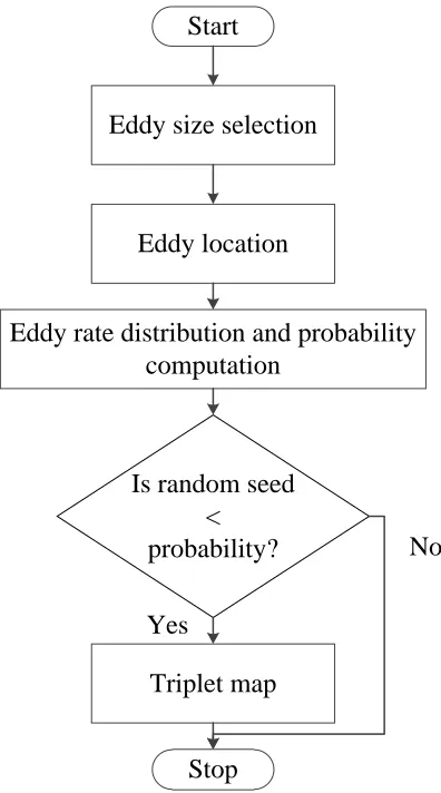
for modeling turbulence is given in Figure 3.1.
Start
Eddy size selection
Eddy location
Eddy rate distribution and probability
computation
Is random seed
<
probability?
Triplet map
Stop
No
Yes
3.4.1 Eddy Size Determination
The eddy length scale, l, is sampled from a distribution function given by Eq. 3.7.
f(l) = A
l2 (3.7)
where A is a constant. Letsminandsmaxbe the smallest and largest eddy sizes. The integration
of the distribution function from smin tosmax should result 1.
Z smax
smin
f(l) dx= 1 (3.8)
From Eq. 3.7 and Eq. 3.8, we get
A= sminsmax
smax−smin
(3.9)
The length distribution can thus be written as
f(l) = sminsmax
smax−smin 1
l2 (3.10)
3.4.2 Eddy Location Determination
The eddy location is based on a uniform distribution function on the ODT domain. The
distribution function corresponding to a locationy0 is given by Eq. 3.11.
g(y0) = 1
LODT
(3.11)
3.4.3 Eddy Rate Distribution
The eddy rate distribution, λ, governs the rate of eddy events in ODT. It is a function of the
eddy length scaleland eddy locationy0. It is associated with a time scale τ which is based on the instantaneous velocity field.
λ(t;y0, l) =
C l2τ(t;y
0, l)
(3.12)
In Eq. 3.12,C is a constant that represents the turbulent intensity.
3.4.4 ODT Acceptance Probability
The acceptance probability determines whether or not an eddy event occurs. It is the ratio of
the desired probability to the presumed probability. In order to determine whether or not an
eddy event occurs, a random number is chosen and compared to the acceptance probability.
The event is accepted if it is less than the probability. The acceptance probability is evaluated
based on the eddy rate distribution normalized by the probability density functions of location
and eddy size [8].
Pa=
λ(t;y0, l) ∆ts
f(l)g(y0)
(3.13)
In Eq. 3.13, ∆ts is the time step between successive eddy events.
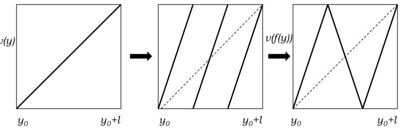
3.4.5 The Triplet Map
Turbulence is implemented in ODT by a mapping procedure known as triplet maps, which
modifies the scalar and vector field along the 1D domain. The triplet map satisfies the
triplet map is defined according to Eq. 3.14 [18].
f(y)≡y0+
3(y−y0) ify0 ≤y≤y0+13l 2l−3(y−y0) ify0+13l≤y≤y0+ 23l 3(y−y0)−2l ify0+23l≤y≤y0+l
y−y0 otherwise
(3.14)
In Eq. 3.14, f(y) is the mapping function,y0 is the starting location of the eddy, and l is the eddy length scale. The effect of triplet mapping on a scalar field along an ODT domain is
shown in Figure 3.2. A segment of the ODT domain corresponding to an eddy location and
size is shown. The initial scalar field is compressed to one-third its original extent, and two
additional copies are made. These are arranged as shown in the figure, and then the middle
copy is inverted. This is done to mimic the effect an eddy has on the scalar field.
y0 y0+l y0 y0
v(y) v(f(y))
y0+l y0+l
Figure 3.2: Effect of the triplet map on a scalar field.
A discrete version of triplet map is implemented in the current study. For this the number
defined by Eq. 3.15 [22].
f(j)≡j0+
3(j−j0) ifj0≤j≤j0+13ke 2ke−3(j−j0) ifj0+ 13ke≤j≤j0+23ke 3(j−j0)−2ke ifj0+ 23ke≤j≤j0+ke+ 1
j−j0 otherwise
(3.15)
In Eq. 3.15,f(j) is the discrete mapping function, j is the grid location,j0 is the starting grid location of the eddy, and keis the discrete eddy size. The eddy size is thusl=ke∆xODT.
3.4.6 The Pressure-Scrambling Model
In buoyant stratified flows, triplet mapping of density may alter the total potential energy
while leaving the kinetic energy unchanged [36]. The energy conservation is enforced by adding
a kernel transformation function to the velocity field so that the total energy is conserved. The
kernel transformation funcionK(y) is added to each component of velocity as given in Eq. 3.16.
ui(y)→ui(f(y)) +ciK(y) (3.16)
Here, ci is the amplitude given by Eq. 3.18. The kernel transformation function is given by
Eq. 3.17.
K(y)≡y−f(y) (3.17)
ci = 27 4l
−ui,K+ sgn(ui,K) s
u2i,K+α0 X
j
Tiju2j,K
(3.18)
In Eq. 3.18,α0 represents the maximum allowable energy that is to be exchanged and 0< α0< 1. α0 = 0 results in no exchange of energy while α0 =
2
in all three directions. T is a the transfer matrix defined as:
T ≡ 1 2
−2 1 1
1 −2 1
1 1 −2
(3.19)
3.5
Computation of Scalars
The fine grid resolution of ODT permits the use of the actual value of the scalar parameters
such as viscosity and thermal conductivity. This is in contrast to LES where these parameters
have to be modeled to take into account the subgrid scale effects. The evaluation of these
parameters in ODT is taken to be the same as that FDS uses in DNS mode.
3.5.1 Viscosity
The viscosity computation is given by Eq. 3.20 [27] [2].
µβ =
26.69×10⁻⁷(WβT)
1 2
σ2 βΩv
kg
m·s (3.20)
Wβ is the molecular weight of speciesβ,T is the temperature, and Ωv is the collision integral
given by Eq. 3.21. exp
Ωv = 1.6145(T∗)−0.14874+ 0.52487e−0.7732T
∗
+ 2.16178e−2.43787T∗ (3.21)
T∗= kB
T (3.22)
σβ and are the Lennard-Jones potential parameters with units of length and energy
respec-tively. kB is the Boltzmann constant. The effective viscosity of the gaseous mixture is given
as:
µ=X β
whereYβ is the mass fraction of speciesβ.
3.5.2 Mass Diffusivity
Mass diffusivity is a function of temperature and the species. The diffusion coefficient of species
α intoβ is given by Eq. 3.24. It has been assumed that all species diffuse into nitrogen.
Dαβ =
2.66×10⁻⁷T32 W
1 2
αβσ2αβΩD
m2
s (3.24)
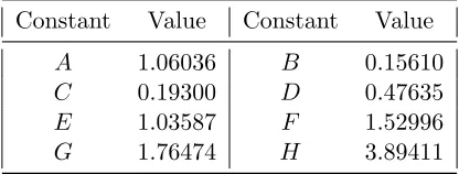
ΩD is the diffusion collision integral given by Eq. 3.27 [27].
σαβ = σα+σβ 2 (3.25) 1 Wαβ = 1 2 1 Wα + 1 Wβ (3.26)
ΩD =
A
(T∗)B +
C
eDT∗ + E
eF T∗ + G
eHT∗ (3.27)
The constants used in Eq. 3.27 is given Table 3.1.
Table 3.1: Constants used in the calculation of ΩD
Constant Value Constant Value
A 1.06036 B 0.15610
C 0.19300 D 0.47635
E 1.03587 F 1.52996
G 1.76474 H 3.89411
3.5.3 Thermal Conductivity
The thermal conductivity for a speciesβ is calculated based on the viscosity (µβ), specific heat
and a value of 0.7 is used.
kβ =
µβcp,β Pr
W
m·K (3.28)
The thermal conductivity of the gaseous mixture is calculated in a manner similar to that of
viscosity.
k=X β
Yβkβ (3.29)
3.5.4 The Density
The density of each species is calculated using the ideal gas relation given in Eq. 3.6. The
pres-sure is constant while the mass fraction and temperature are governed by the ODT equations.
The mixture density is given by Eq. 3.30.
ρ= p
RuTX
β
Yβ
Wβ
(3.30)
where Ru is the universal gas constant.
3.5.5 The Chemical Reaction Rate
A simple propane-air reaction as show in Eq. 3.31 is considered. The reaction rate is calculated
using the Arrhenius equation, and the mass productoin rates are calculated as in Eq. 3.31 –
Eq. 3.32.
˙
m000F =−B χFχO2e
Ea
RuT (3.31)
˙
m000O2 = 5 ˙m000FWO2 WF
(3.32)
whereχis the mole fraction,Bis the pre-exponential factor, andEais activation energy. These
Chapter 4
LES-ODT Coupling
4.1
Objective
Chapters 2 and 3 discussed the LES and ODT models. This chapter discusses the
imple-mentation details of the coupling between the two models. The specialities of the Lagrangian
approach to coupling is discussed along with the flow of information between LES and ODT.
Interpolation, filtering and management of ODT domains are discussed in this chapter.
4.2
LES-ODT Coupling – Lagrangian Formulation
As mentioned before, a Lagrangian formulation has been adopted for coupling between the LES
and ODT models in this study. In this approach, the ODT elements are attached to the flame
surface and they exist only in the vicinity of the flame brush. As the flame evolves, the ODT
elements attached to the flame move with them. This is in contrast to the Eulerian approach
[4] in which the ODT elements are embedded throughout the computational domain and are
stationary. Figure 4.1 and Figure 4.2 show the arrangement of the ODT domains on the flame
brush.
The objective of formulating such a model is to decouple the computation of the non-reacting
the small scale effects in a flame such as chemistry. This is a flame-embedding technique in
which the ODT solution provides closure to the LES equations.
Flame surface (obtained by transporting the mixture fraction in LES) ODT domains
Figure 4.1: Embedding strategy: The ODT domains attached to the flame brush. The orien-tation of domains is normal to the flame surface.
The ODT domains are attached to the flame brush and are oriented normal to the flame
surface. This can be compared to the Eulerian approach show in Figure 1.1. The flame surface
is determined from LES based on the mixture fraction field. It is the isosurface corresponding
to the stoichiometric mixture fraction (Zf). The ODT domains have anchor points, which are
in the middle of each ODT domain. These anchor points are attached to the flame surface.
As the flame evolves the anchor points follow it while maintaining their orientation normal to
the flame surface. As shown in Figure 4.2, the ODT domains traverse multiple LES grid cells.
Each LES cell through which a flame surface passes has at least one ODT domain.
Since much of the chemistry effects reside around the flame surface, higher resolution is
desired in this region. In the Lagrangian approach, the high resolution ODT grids exist only
around the flame surface. This method obviates embedding ODT elements in other regions
where they are not required as much, hence reducing computational cost. This allows simulation
LES domain (coarse grid)
LES cell ODT domain
Flame surface
Figure 4.2: Embedding strategy: ODT domains in an LES grid
of the solution. Also, since the domains are stationary relative to flame convection terms are
removed from the governing equations.
4.3
LES-ODT Information Exchange
During the initialization time step, velocity and mixture fraction are interpolated from LES
into ODT using tri-linear interpolation. Temperature and mass fractions on ODT grid points
are calculated from the mixture fraction. The solution parameters of ODT governing equations
are hence velocity, temperature and mass fractions. At the subsequent time steps, the ODT
velocity is replaced by the filtered velocity field from the LES solution interpolated from LES
into ODT and the residual term from the ODT solution, while the scalar solutions are advanced
using the existing thermo-chemical scalar profiles. The densities obtained from ODT solutions
is spatially filtered into LES grid. The filtered density replaces LES density. This is illustrated
in Figure 4.3.
4.4
Interpolation
The parameters on LES grid including the velocity field and mixture fraction are passed on to
Velocity
Large Eddy
Simulation
One Dimensional
Turbulence
Filtered density
Figure 4.3: Exchange of information between LES and ODT
scalar field is assumed, and this method is an extension of the linear interpolation and bilinear
interpolation [29] to three dimensions. The interpolation of a scalar parameter is discussed in
this section, and its implementation for a vector is obvious as a vector can be treated as three
different scalars.
The interpolated value in each ODT grid point is based on the nodal values of the rectilinear
LES cell within which it is located. This is shown in Figure 4.4 where a scalar parameter is
interpolated from the nodes of the cube on a point in the cube. The interpolation is given by
Eq. 4.1, where f is the scalar parameter on an LES grid node and ginterp is the interpolated
value on an ODT grid point. Velociy and mixture fraction are interpolated using this method.
ginterp= (1−α)(1−β)(1−γ)fi,j,k + ( α)(1−β)(1−γ)fi+1,j,k + (1−α)( β)(1−γ)fi,j+1,k
+ (1−α)(1−β)( γ)fi,j,k+1 (4.1) + (1−α)( β)( γ)fi,j+1,k+1
zc
z0
xc x0
yc
x y z
Cartesian grid points
y0
Interpolation point
(i,j,k)
(i+1,j+1,k+1)
The parametersα,β and γ used in Eq. 4.1 are defined as:
α = x0 xc
; β = y0
yc; γ = z0 zc
(4.2)
4.5
Initialization of Scalar Parameters
The solution parameters of the ODT governing equations are velocity, temperature and mass
fractions. Velocity is interpolated from LES grid at each time step. Temperature and mass
fractions of fuel and oxygen are calculated based on the interpolated mixture fraction only
at initialization of ODT domains. The relation between mixture fraction and ODT scalars is
shown in Figure 4.5.
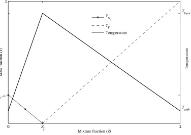
0 1
1
Mixture fraction (Z)
Mass fraction (
Y ) Temperature Y O 2 Y F Temperature T burn T amb Y O
2, air
Zf
Figure 4.5: State relation: Initialization of ODT scalars from the mixture fraction.
for pure oxidizer. For a premixed flame, it can used as a flame surface marker where the flame
brush corresponds to the stoichiometric mixture fraction (Zf). For a propane-air reaction,
Zf = 0.059. Infinitely-fast chemistry is assumed such that fuel and oxygen are completely
consumed at the flame surface. However, it is to be noted that this assumption is only during
initialization and ODT solutions do exhibit finite-rate chemistry effects. On the fuel side, the
fuel mass fraction (YF) varies from 1 forZ = 1 to 0 for Z =Zf. The temperature on the fuel
side varies from the fuel inlet temperature, which is assumed to be the same as the ambient
temperature (Tamb), for Z = 1 to the adiabatic flame temperature (Tburn) for Z =Zf. On the
oxidizer side, the oxygen mass fraction goes from 0 for Z =Zf to the mass fraction value for
oxygen in pure air (YO2,air) forZ = 0. The temperature again varies from Tburn atZ =Zf to
the ambient temperature atZ = 0.
4.6
Management of ODT Domains
Since the ODT domains are not fixed, managing the location and orientation of the ODT
domains is an important aspect of the modeling framework. The flame surface is determined
from the LES solution based on the stoichiometric mixture fraction. The ODT domains are
attached to the flame surface along anchor points which lie on the center of the domains as
shown in Figure 4.6. As the domains are transported with the flame, the domains have to be
redistributed to maintain a uniform distribution.
4.6.1 Flame Displacement Speed
The ODT elements are oriented normal to the flame surface. At each LES time step, the
flame surface changes and new location of the anchor point is determined as well the new
normal. The ODT domains are then moved to this location and their orientation changed. The
displacement of the anchor points is given by Eq. 4.3, where ˜ui is the filtered flow velocity and
xi is the location of the anchor point.
dxi
Flame brush
(stoichiometric
mixture fraction)
Previous
orientation
New domain
orientation
Anchor point
Figure 4.6: Anchoring and transport of ODT domains.
Eq. 4.4 gives the unit vector that is normal to the flame surface. It is the direction of
maximum gradient of the mixture fraction scalar field. Since the discrete scalar field is located
at the cell centers, the gradients at the cell centers are first calculated. The gradient value at
the anchor points are then calculated by interpolation as described in Section 4.4.
ˆ
n= ∇Z
|∇Z| (4.4)
whereZ is the mixture fraction.
4.7
Filtering
As shown in Figure 4.3, the values of density for cells around the flame calculated from ODT
are provided into LES. LES cells around the flame surface have a number of ODT grid points
in their vicinity. The ODT grid resolution is much finer than LES and as such any ODT data
supplied has to be spatially filtered.
A method for filtering based on distance-weighted kernel functions around the ODT domains
is discussed in this section. This method is currently used in the code. However, in this method
RBF interpolation is studied and is discussed in Section 5.7. An introduction to RBF is included
in Appendix A. At its current stage, the RBF method is determined to be not feasible in our
case. With some modifications that is still a subject of research, it could potentially be used as
a filtering method.
We proceed to describe the distance weighted method used in filtering scalar parameters
from ODT grids to LES grid.
4.7.1 Region of Influence of Domains
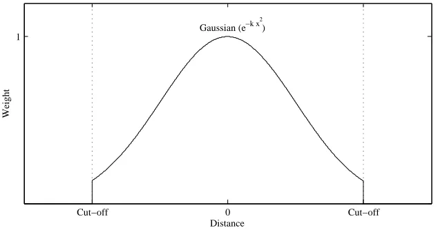
For the filtering process, the ODT domains are thought to be having a region of influence
around them. The influence of the domain in this region is given by a kernel function (G(r))
which is a function of the perpendicular distance of a point from the line consisting the ODT
domain. In the present study, this kernel function is a clipped Gaussian with a cut-off at a
distance as shown in Figure 4.7.
Cut−off 0 Cut−off
1
Distance
Weight
Gaussian (e−k x
2
)
Figure 4.7: Kernel function used in the filtering process as a function of distance.
It should be noted that the solution parameters in ODT domains are not deterministic but
stochastic. The ODT domain is divided into smaller segments and an average value is calculated
Figure 4.8.
ODT Domain
Scal
ar
V
al
ue
Actual value
Averaged value
Figure 4.8: Averaging the data on an ODT domain.
The region of influence of the domains can be visualized as a set of cylinders as shown in
Figure 4.9 with weight distribution given by the kernel functionG(r).
ODT Domain
LES Cell
4.7.2 Method of Cubature
The filtered value for a scalar parameter (density in the present case) within an LES cell is
calculated as a volume averaged value given by Eq. 4.5. The method of cubature is used to
numerically evaluate a multivariate integral [19].
¯
ρ= Z Z Z
cell ˆ
ρ(x) dV
Z Z Z
cell dV
(4.5)
The integration is done throughout the volume of the LES cell and x is the coordinate of a
point within the cell. ˆρ is a value based on the influence of ODT domains given by Eq. 4.6.
ˆ
ρ(x) = X
ODT
G(r)ρavg
X
ODT
G(r) (4.6)
The summation is done for all the ODT domains influencing the pointx. r is the perpendicular
distance from the point to the ODT domain. ρavg is the average scalar value in the segment
influencing x.
4.7.3 Implementation
The volume integral for each LES cell is calculated by dividing the cell into a number of identical
smaller sub-divisions. The ˆρ values for each of these sub-divisions is calculated and then the
average taken.
When calculating ˆρ in Eq. 4.6 the most direct way would be to calculate the influence of
each domain on a particular point. However, in a typical simulation scenario the number of
ODT points are of the order of a few thousands and the LES cells of a million. Also, the points
further away do not have an influence as the kernel function has a cut-off beyond a certain
point. The direct method would be unnecessarily costly. Hence, for each point evaluation is
LES cell within which it is located. During evaluation, only the domains close to the LES cell
are considered.
The selection of a number of parameters influence the result of the filtering method. These
include the shape of the kernel function and the number of sub-divisions within an LES cell.
Taking a large number of sub-divisions increases the computational cost and an optimal value
has to be chosen. Imcreasing the span of the kernel function, a Gaussian curve, results in
reduction of peak values. But a span too narrow results in a solution where the filtered cells are
not contiguous. The selection of these values is done by making trial runs and selecting values
Chapter 5
Simulation Condition and Results
A sample simulation using the proposed LES-ODT coupled model is performed. The simulation
condition including some results have been demonstrated and explained in this chapter. This
chapter discusses the results of the simulation of a non-premixed propane-air jet flame using
the LES-ODT coupled model with a Lagrangian formulation.
5.1
Overview
A flame-embedding framework for simulation of a non-premixed flame is described in the
pre-vious chapters. In this chapter, some of the steps involved in the formulation of the model
are demonstrated. These include managing the ODT domains on the flame surface (Section
5.5) and filtering of scalar parameters (Sections 5.6 and 5.7). The specifications of the sample
simulation performed are illustrated in Section 5.2. The simulation results on a sample ODT
domain are given in Sections 5.3 and 5.4 in which the capabilities of the model to predict
phe-nomena such as flame wrinkling and turbulence-chemistry interacitons can be seen. Finally,
5.2
Simulation Condition
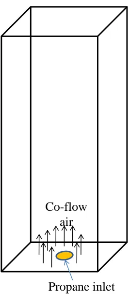
A non-premixed flame consisting of propane (C3H8) as fuel and air as oxidizer is simulated. The computational domain is a rectangular box open to the atmosphere on all sides except the
bottom as shown in Figure 5.1. A fuel inlet of diameter 10 mm is at the center of the bottom
surface which supplies propane at a speed of 1 m/s. The fuel inlet is surrounded by co-flow air
at a speed of 0.5 m/s.
Propane inlet
Co-flow
air
Figure 5.1: Computational domain used in the simulation.
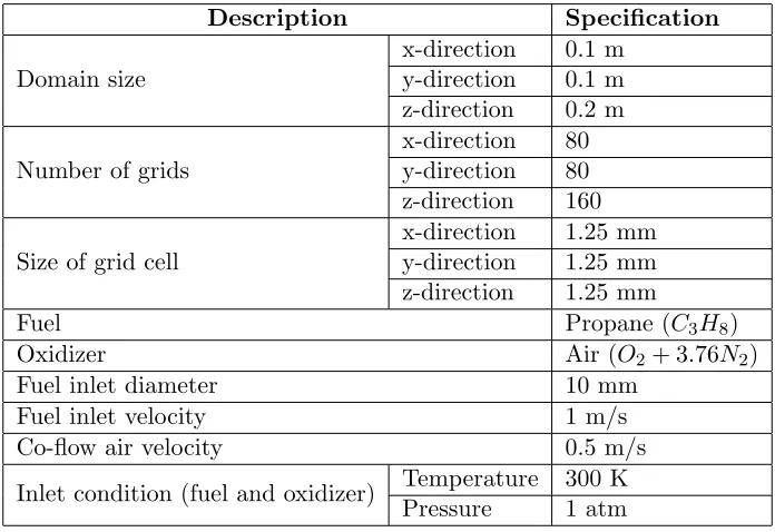
The domain is divided into uniform rectilinear grid cells. The grid size is constant within
each dimension but may vary between dimensions. Table 5.2 shows some of the parameters
Table 5.1: Simulation condition: Description of the LES domain.
Description Specification
Domain size
x-direction 0.1 m y-direction 0.1 m z-direction 0.2 m
Number of grids
x-direction 80 y-direction 80 z-direction 160
Size of grid cell
x-direction 1.25 mm y-direction 1.25 mm z-direction 1.25 mm
Fuel Propane (C3H8)
Oxidizer Air (O2+ 3.76N2)
Fuel inlet diameter 10 mm
Fuel inlet velocity 1 m/s
Co-flow air velocity 0.5 m/s
Inlet condition (fuel and oxidizer) Temperature 300 K Pressure 1 atm
At the beginning of simulation the model is run with only the LES formulation existing
in the FDS model (i.e. without ODT). After the flame has reached a sufficient height, ODT
domains are introduced and the ODT simulation is started. Table 5.2 shows the parameters
related to the ODT domain.
Table 5.2: Simulation condition: Description of the ODT domains.
Description Specification
ODT domain length 16 mm
Number of ODT grids 41
ODT grid size 0.4 mm
5.3
ODT Solutions of Scalar Parameters
The scalar parameters on ODT grid are the temperature, the fuel mass fraction and the oxidizer
mass fraction. As mentioned earlier, these are initialized from the mixture fraction based on
the state relations shown in Figure 4.5. On initialization, there is one peak temperature, fuel
mass fraction is zero on the oxidizer side, and oxygen mass fraction is zero on the fuel side. An
example of the effects of the ODT governing equations on these scalar parameters can be seen
in Figure 5.2 – Figure 5.4.
The effect of turbulence and finite-rate chemistry can be seen in these plots. Multiple peak
tempertures caused by the stirring events can be seen which results in flame wrinkling. Also,
it can be seen that the fuel and oxygen can coexist at a point, which demonstrates the effect
of finite-rate chemistry.
ODT Grid Position
T
e
m
p
e
ra
tu
re
(K
)
10 20 30 40 0
500 1000 1500 2000
ODT Grid Position F u e l M a s s F ra c ti o n (Y f)
10 20 30 40 0 0.02 0.04 0.06 0.08 0.1
Figure 5.3: Fuel mass fraction on an ODT domain.
ODT Grid Position
O x y g e n M a s s F ra c ti o n (Y o )
10 20 30 40 0
0.05 0.1 0.15 0.2
5.4
Finite-Rate Chemistry Effects
ODT introduces finite-rate chemistry effects where fuel and oxygen can diffuse into each other
and reaction rate is dictated by the Arrhenius equation (Eq. 3.31). This effect can be seen in
Figure 5.5 where temperature on ODT grid points is plotted against mixture fraction. The
color map is based on the gradient of filtered mixture fraction. As can be seen from the figure,
temperature for the same mixture fraction decreases with increasing gradient. This may result
in lower temperature and eventually flame extinction at locations with high gradient. This
demonstrates the ability of the model to show the effect of finite-rate chemistry effects and
turbulence.
Figure 5.5: Effect of turbulence and finite-rate chemistry on temperature.
5.5
Addition and Redistribution of ODT Elements
The number of ODT domains used in the simulation changes at each time step. When ODT
elements are first introduced into the domain, they are uniformly distributed on the flame
surface. As the flame gets larger and changes shape, the ODT domains follow it. A growth
and compression of the flame surface results in an uneven distribution of ODT elements. If
not corrected, this leads to clustering of domains in some locations and sparse distributions in
others as shown in Figure 5.6.
Cluster Sparse
Figure 5.6: Unveven distribution of ODT elements when not corrected.
Also, as the flame grows the ODT domains tend to move to the flame tip. The domains
leave the flame surface once they reach the flame tip as can be seen in Figure 5.7. These “stray”
domains are removed and are replaced by newer elements.
In order to ensure a uniform distribution of domains, they are redistributed at each LES
cycle. Every LES cell that is on the flame must have at least one ODT domain in it. A
minimum and a maximum number of domains that each cell on the flame can have is fixed.
If a cell has too many domains they are removed, and if it has too few domains newer ones
are added. Besides, for the mixture fraction corresponding to the anchor points on each ODT
domain, a minimum and a maximum values are fixed. Any domain for which this is beyond the
range is removed making sure “stray” domains do not exist. Figure 5.8 shows the arrangement
of domains on the flame after correction has been made.
Figure 5.7: ODT elements leaving the flame surface from the flame tip.
X Y Z
on them as discussed in Section 4.5. The filtered velocity and mixture fraction are first
inter-polated on ODT domains. The ODT scalar parameters – temperature, fuel mass fraction and
oxygen mass fraction – are initialized from mixture fraction using the state relations.
5.6
Filtering Process
Density is calculated from the temperature and mass fractions on the ODT domain. This is
then filtered and the filtered density is stored at the LES cell centers. The filtered density
replaces the density calculated in FDS. The filtering method used is described in Section 4.7,
the results of which are discussed in this section. Apart from this, another method using radial
basis functions has been investigated, which is described in Section 5.7.
Since the ODT domains exist only around the flame, filtered density is used only for cells
that are in the neighborhood of the flame. Figure 5.9 – Figure 5.10 show the filtered density
and density generated from FDS. The latter is the density used in the LES model. These
are shown here for comparison. The filtered density is overlayed on the LES density, so LES
density is shown in cells where a filtered value does not exist. The density in ODT is lower
than that of LES since the temperature is higher in ODT. Besides, the filtering process is an
averaging process and hence reduces peak values. We can see in the figures that the LES-ODT
filtered density does exhibit the expected trends in the flame which corresponds to a reduction
in density. However, the filtered density contours may need to be smoothed using a recursive
filter, such as a Kalman filter, given the potentially-noisy nature of filtering stochastic densities.
Figure 5.11 shows the LES grid cells to which filtered density is passed. These cells surround
FDS Density
X Y
Z 2 1.6 1.2 0.8 0.4 0.1
Filtered Density
kg/m^3
Figure 5.9: Filtered density and FDS density in x-plane.
FDS Density
X Y Z
2 1.6 1.2 0.8 0.4 0.1
Filtered Density
kg/m^3
Figure 5.10: Filtered density and FDS density in y-plane.
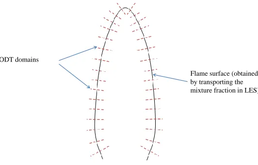
Full
X Y Z
Half-section
![Figure 1.1:Schematic of LES-ODT coupling using Eulerian approach [4]. ODT elements inonly one direction have been shown.](https://thumb-us.123doks.com/thumbv2/123dok_us/1596117.1196992/15.612.185.442.486.617/figure-schematic-coupling-eulerian-approach-elements-inonly-direction.webp)