University of Windsor University of Windsor
Scholarship at UWindsor
Scholarship at UWindsor
Electronic Theses and Dissertations Theses, Dissertations, and Major Papers
2011
Source Node Expansion Algorithm for Coherency Based Islanding
Source Node Expansion Algorithm for Coherency Based Islanding
of Power Systems
of Power Systems
Issah Ibrahim
University of Windsor
Follow this and additional works at: https://scholar.uwindsor.ca/etd
Recommended Citation Recommended Citation
Ibrahim, Issah, "Source Node Expansion Algorithm for Coherency Based Islanding of Power Systems" (2011). Electronic Theses and Dissertations. 129.
https://scholar.uwindsor.ca/etd/129
This online database contains the full-text of PhD dissertations and Masters’ theses of University of Windsor students from 1954 forward. These documents are made available for personal study and research purposes only, in accordance with the Canadian Copyright Act and the Creative Commons license—CC BY-NC-ND (Attribution, Non-Commercial, No Derivative Works). Under this license, works must always be attributed to the copyright holder (original author), cannot be used for any commercial purposes, and may not be altered. Any other use would require the permission of the copyright holder. Students may inquire about withdrawing their dissertation and/or thesis from this database. For additional inquiries, please contact the repository administrator via email
SOURCE NODE EXPANSION ALGORITHM FOR COHERENCY
BASED ISLANDING OF POWER SYSTEMS
by
Issah Ibrahim
A Thesis
Submitted to the Faculty of Graduate Studies
through the Department of Electrical and Computer Engineering
in Partial Fulfillment of the Requirements for
the Degree of Master of Applied Science at the
University of Windsor
Windsor, Ontario, Canada
2011
iii
AUTHOR’S DECLARATION OF ORIGINALITY
I hereby certify that I am the sole author of this thesis and that no part of this thesis has
been published or submitted for publication.
I certify that, to the best of my knowledge, my thesis does not infringe upon anyone’s
copyright nor violate any proprietary rights and that any ideas, techniques, quotations, or any
other material from the work of other people included in my thesis, published or otherwise, are
fully acknowledged in accordance with the standard referencing practices. Furthermore, to the
extent that I have included copyrighted material that surpasses the bounds of fair dealing within
the meaning of the Canada Copyright Act, I certify that I have obtained a written permission
from the copyright owner(s) to include such material(s) in my thesis and have included copies of
such copyright clearances to my appendix.
I declare that this is a true copy of my thesis, including any final revisions, as approved by
my thesis committee and the Graduate Studies office, and that this thesis has not been submitted
iv ABSTRACT
The electric power system is an exposed man-made structure susceptible to wide arrays of
disturbance. If not cleared, a lingering disturbance can plunge the system into the unstable mode
in a fairly short time frame.
In distributed generation, a drawn-out perturbation can cause system components to
operate under unacceptable conditions. When restoration controls fail to revive the troubled
system, generators may lose synchronism causing them to swing haphazardly in groups. This
crisis separates the power system into unbalanced regions called unintentional islands.
In this thesis, Source Node Expansion Algorithm based on Slow Coherency has been
proposed to resolve unintentional islanding. The algorithm initiates expansion from source node,
engulfs connected loads until desired power mismatch is met. It then terminates and optimal
cutsets deduced from the Adjacency Matrix.
The proposed technique is tested on 14 and 37-bus systems to endorse its potency. The
experimentation is carried out in the PowerWorld platform.
v
ACKNOWLEDGEMENTS
I wish to express my utmost gratitude to my advisor, Dr. M. Sid-Ahmed, for his endless
support, ideas, perspectives, and artful encouragement during my two-year stint as a graduate
student at the University of Windsor.
I also owe an incalculable debt of gratitude to my co-advisor, Dr. Ali Tahmasebi, who
does the work of ten men and seemly enjoys every minute of it. His passion for ideas, his
formidable knowledge, and his balance between academic life and everything else have been
inspirational. He has showed me, and continues to show me crucial mentorship and guidance
throughout my research. Thank you, Tahmasebi.
The following people deserve thanks for agreeing to be part of my defense committee: Dr.
N. Kar, Electrical and Computer Engineering department; Dr. D. Ting, Mechanical Engineering
department; and Dr. J. Wu for emceeing my thesis defense. Their painstaking review of my
work, their comments and suggestions were very useful in the final redaction of this thesis.
I would also like to thank the University of Windsor Electrical and Computer Engineering
Department especially, Ms. Andria Ballo, Graduate secretary extraordinaire, for her unflinching
support and assistance with all the paper works.
Finally, a lot of thanks go to my family and friends in Canada whose contribution have
brought my master’s experience to fruition, and those outside who refreshingly have no idea
vi
TABLE OF CONTENTS
AUTHOR’S DECLARATION OF ORIGINALITY…………..……….……….………….iii
ABSTRACT ………...…….………...………...……iv
ACKNOWLEDGEMENTS ………..………..……….….…………..…v
LIST OF TABLES………..………..……….….……...…….ix
LIST OF FIGURES ………...….……x
CHAPTER 1 Introduction 1.1 Electric Power System ………...…….…1
1.1.1 Transmission System ……….…………....2
1.1.2 Sub-Transmission Level ….……….………….….…3
1.1.3 Distribution System ……….….….3
1.1.4 Utilization……….……....……….…4
1.2 Electric Power System Representation……….…..……….………4
1.3 Forms of Electric Power System ……….…...…….6
1.3.1 Centralized Generation System ………...……….……...…..6
1.3.2 Distributed Generation System ……….……...…….9
1.3.3 Technologies used for Distributed Generation……..…..…...……..10
1.3.4 Benefits of Distributed Generation ……….…………...…11
1.3.5 Challenges of Distributed Generation ………….………....….12
CHAPTER 2 Islanding Concept 2.1 How Islands are Formed …………...…….……..….…….…..…..……...…..15
2.2 Issues Related to Islanding ……….……..….…….……….…..…..……16
2.3 Islanding Detection Techniques………….……….……….16
2.3.1 Remote Detection Technique ………..…….………17
vii CHAPTER 3 Literature Review
3.1 Controlled Islanding ……….…....……….22
3.2 Coherency Identification of Generators ………23
3.2.1 Slow Coherency Method ……….……….24
3.3 Graph Theory….………...…….………25
3.3.1. Graph Generation ………....……….26
3.3.2 Graph Simplification ………..…………..27
3.3.3 Graph Partitioning ………29
3.4 Graph Searching Algorithms….………....………29
3.4.1 Classical Dijkstra Algorithm………...………...29
CHAPTER 4 Source Node Expansion Algorithm 4.1 How the Algorithm works……..………...……….….…….32
4.1.1 Generator Grouping………..….….………32
4.1.2 Transport Network……….………...………...…….……..32
4.1.3 Dijkstra Implementation……….………..………….………….…....33
4.1.4 Adjacency Matrix Formation……….…..………..………….………35
4.1.5 Source Node Expansion Using Adjacency Matrix…..……….……..36
4.1.6 Final Separation……....……….………...…....…..39
CHAPTER 5 Case Study 5.1 The 14-bus System ………..…..………...…….40
5.1.1 System Design………..………….…………...40
5.1.2 The 14-Bus Graph Model ……….……….…………..……40
5.1.3 Fault Analysis ………..………41
5.1.4 Simulation Results ………..….42
5.1.5 Cutset Search ……….…..45
5.1.6 Final Separation ……….………..…47
5.1.7 Bus Voltage Comparison ………..………...……48
5.2. The 37-Bus System ……….………..………51
viii
5.2.2 The 37-Bus Graph model ………...…………..……...52
5.3 Fault Analysis ………...………….54
5.3.1 Contingency 1 ………...…………54
5.3.2 Simulation Results ………..………..……….….55
5.3.3 Contingency 2 ………..…….…..57
5.3.4 Simulation Results ………...………..…….…58
5.3.5 Contingency Resolution ………..……….…..59
5.3.6 Final Separation ……….………..……….…..62
5.3.7 Simulation Results………..……….…63
CHAPTER 6 Discussion and Conclusion 6.1 Future work to be done.………...……….66
APPENDICES Appendix A1……….………..……….……….67
Appendix A2………..……...………68
Appendix A3………...……..………...………69
REFERENCES……….……….………...………..70
ix
LIST OF TABLES
Tables
1.1. Voltage Hierarchy ………..……….2
1.2. Component and symbols ……….………….…….…..5
1.3. Historic Blackouts Data ……….…….……7
1.4. T&D Losses & Unaccounted for Electricity in the US ……….….…….…8
4.1. Grouping Data ……….…..……33
4.2. Dijkstra Output ……….………...……..35
4.3. Generation-Load Mismatch Data ……….……….39
5.1. Load Information ……….………...……..41
5.2. Generator Information ……….……...……..41
5.3. Dijkstra Results ……….…….……..………….46
5.4. Adjacency Matrix ……….………...………..47
5.5. Bus Voltages ………..……….……..………48
5.6. Bus Information ………...……….………...………….53
5.7. Adjacency Matrix ……….……….61
x
LIST OF FIGURES
Figures
1.1. Electric Power System ………..………..1
1.2. Single Line Diagram……….……….…………..6
1.3. One Line Diagram of a Distributed Generation System……….……….9
2.1. Islanding Operation ……….…………..14
2.2. Generator Speed after Contingency ……….…...………..15
2.3. Bus Voltage Magnitude after Contingency ……….……..………15
2.4. Islanding Detection Techniques ……….………...………17
2.5. Power Line Carrier Communication ………..………...………18
3.1. Swing Curve of a 56-Bus System ………....…….………24
3.2. Swing Trajectories of 15,549 Bus System ……….….………..25
3.3. Removal of Degree-one Node ……….………….27
3.4. Removal of Degree-two Node ……….……….27
3.5. A 6-Bus System ………..…………..………28
3.6. A 4-Bus Graph Model….……….…....………..28
3.7. Graph size before and after Reduction ………...……..…….………28
3.8. A Directed Graph….………...……….………..30
4.1. SNE Flow Chart…..……….…………..………31
4.2. 16-node Transport Network..……….……….……..….33
4.3. Dijkstra Algorithm on 16-node Transport Network..……….……….…..……34
4.4. Adjacency Matrix of 16-node Transport Network …...……...….…....…………..…..36
4.5. SNE of Adjacency Matrix and Cutsets…...……….…………...………37
4.6. Balanced Islands in the 16-node Transport Network ………..….………38
4.7. Balanced Islands ………...………..……….39
5.1. 14-bus System ……….…….40
5.2. Simplified Graph of 14-Bus System ……….….……..41
5.3. Generator Angles after Contingency ………..….42
5.4. Generator 1 Rotor Angle……….………...…...43
xi
5.6. Generator 3 Rotor Angle ……….….…43
5.7. Generator 6 Rotor Angle ……….……….…....43
5.8. Generator 8 Rotor Angle ………..……43
5.9. Generator Speed Deviations after Contingency ……….…..…44
5.10. Bus Voltage Magnitudes after Contingency ……….………….……..…45
5.11. MATLAB Graph ……….……….45
5.12. Marking Cutsets ……….…………..……47
5.13. Removing Cutsets ………..………..……47
5.14. Balanced Islands ………..……...……….48
5.15. 37-Bus System ……….…..……..51
5.16. Simplified Graph of the 37-Bus System ………..…52
5.17. Fault Location on 37-Bus System ………..…………..54
5.18. Generator Rotor angle after Contingency ………..………….…….55
5.19. Bus Speed Deviation after Contingency ……….…….……55
5.20. Generator Speed Deviation after Contingency ………..……….…….56
5.21. Bus Voltage Magnitudes after Contingency ………...……….……56
5.22. Three Phase Fault………...…...57
5.23. Generator Rotor angles after Contingency……….…..………58
5.24. Bus Speed Deviations after Contingency…...……….……….58
5.25. Bus Voltage Magnitudes after Contingency…….………59
5.26. A MATLAB Graph…..……….………60
5.27. Cutset Locations………62
5.28. Balanced Islands…...………..………..62
5.29. Generator Rotor angle after Islanding………...……..………..63
5.30. Generator Speed Deviations after Islanding… …………...….………...…….63
1 CHAPTER 1
INTRODUCTION
1.1. Electric Power System (EPS)
The electric power system was initially developed in the late 1800s and is considered the most significant engineering accomplishment of the 20th century. In 1878, Thomas A. Edison began work on the electric light. His epoch-making invention of the dc generators, then called the dynamos, driven by steam engines to supply an initial load of 30KW for 110V incandescent lighting to 59 customers in a 1-square-mile area at Pearl Street in New York City, marked the beginning of the electricity industry [1].
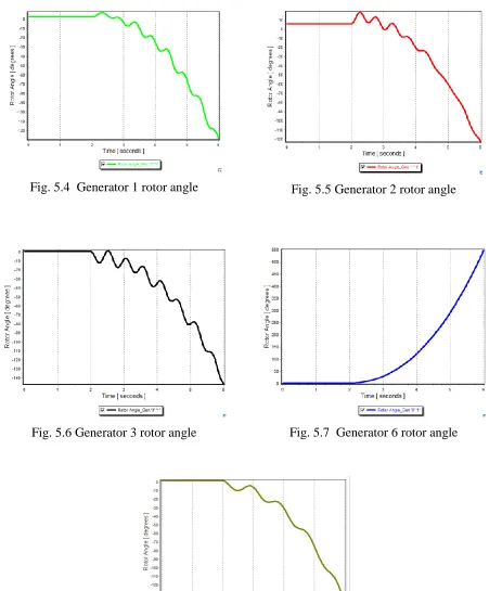
A typical electric power system structure can be divided into four (4) basic subsystems.
a. Generation b. Transmission c. Distribution d. Utilization (Load)
Fig. 1.1 Electric power system
2
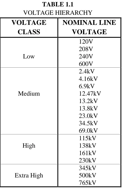
decrease with increasing voltage level. The larger the blocks of power to be transmitted and the greater the distance over which they must be wheeled, the higher operating voltage must be chosen. The U.S standard operating voltages are given in Table 1.1.
TABLE 1.1 VOLTAGE HIERARCHY VOLTAGE CLASS NOMINAL LINE VOLTAGE Low 120V 208V 240V 600V Medium 2.4kV 4.16kV 6.9kV 12.47kV 13.2kV 13.8kV 23.0kV 34.5kV 69.0kV High 115kV 138kV 161kV 230kV Extra High 345kV 500kV 765kV
1.1.1. Transmission System
3
The transmission circuit, unlike the sub-transmission and distribution systems, tends to obtain a loop structure with voltage levels ranging from 115kV to about 765kV. The two general types of power transmission medium are:
a. Overhead Line b. Underground Cable
The most common type of AC power transmission is by overhead conductors suspended from metal towers.
1.1.2. Sub-Transmission Level
The sub-transmission circuit distributes energy to a number of distribution sub-stations in a certain geographical area at a voltage level that typically varies between 23 and 138 kV. It receives the energy directly from the generator bus in a generator station or via bulk power substations. Large customers are served directly from those substations.
The role of a sub-transmission system is mainly the same as that of a distribution system, except that it serves a larger geographical area and distributes energy in larger blocks at higher voltage levels. It should be pointed out that in many systems there are no clear demarcation lines between sub-transmission and transmission circuits. Increased load density makes it necessary and economical to superimpose a new and higher voltage grid on the existing one. In this way yesterday‟s transmission network becomes part of tomorrow‟s sub-transmission network.
1.1.3. Distribution System
The distribution circuits constitute the finest meshes in the overall network. These lines carry limited amounts of power over shorter distances and operate at lower voltages as well. Usually, two distribution voltage levels are used:
1. The Primary or feeder voltage (for instance 23kV)
4
The distribution circuits, fed from the distribution substations (transformer stations), supply energy to the small (domestic) or medium-sized (small industrial and commercial) customers.
1.1.4. Utilization
Loads of power systems are divided into industrial, commercial and residential. Very large industrial loads may be served from the transmission system. Large industrial loads are served directly from the sub-transmission network, and small industrial loads are served from the primary distribution network. The industrial loads are composite loads, and induction motors form a high proportion of these load.
1.2. Electric Power System Representation
Power systems are extremely complicated electrical networks that are geographically spread over very large areas. For most part, they are also three phase networks – each power circuit consists of three conductors and all devices such as generators, transformers, breakers, disconnects etc. are installed in all three phases. In fact, the power systems are so complex that a complete conventional diagram showing all the connections is impractical. Yet, it is desirable, that there is some concise way of communicating the basic arrangement of power system components. This is done by using Single Line Diagrams (SLD). SLDs are also called One Line Diagrams.
5
There is no universally accepted set of symbols used for single line diagrams. Often used symbols are shown in Table 1.2.
TABLE 1.2
COMPONENT & SYMBOLS
NO COMPONENT SYMBOL
1
Generator (Power Station)
2
Transformer (Two winding)
OR
3
Auto-Transformer
4
Current Transformer
5
Circuit Breaker
OR
6
Fuse
7
Disconnect switch
8
Lightning Arrester
OR
9
6
Figure 1.2 shows a small power system. Any information that is required is added to the SLD. In this case connections of generator and transformer windings, as well as the method of grounding the neutral are indicated. This type of SLD has often also specified the size of the equipment in MVAs, voltage levels, and any other relevant information.
Figure 1.2 Single line diagram
1.3. Forms of Electric Power System
The electric utility industry‟s outlook has been greatly influenced by the increasing demand for electricity and the emergence of new generation technologies. This has led to continued restructuring and modification of the conventional EPS structure. The two major forms of EPS are discussed in section 1.3.1 and section 1.3.2 respectively.
1.3.1. Centralized Generation System
The centralized generation paradigm has become the cornerstone of the electricity industry for some time now. It is often referred to as the „archetype‟ of all electric power system structures.
Under this paradigm, electricity is mainly produced at large generation facilities (power plants), shipped through the transmission and distribution grids to load centers. Thomas A. Edison formulated the concept of a centrally located power station in the late 1800‟s.
7
construction, structural and operational drawbacks. The major issues bedeviling the centralized generation system are discussed below.
1. Blackouts:
In power systems, a blackout refers to the total loss of electricity to an area and it is the most severe form of power outage that can occur. Power outages may last from a few seconds to weeks depending on the nature and severity of the blackout and the configuration of the electrical network.
The study of the process of blackouts falls outside the purview of this thesis, but the main cause of their occurrence is major dynamic instabilities following big disturbances. Poor system design, human error, sudden changes to system and many more factors can also play a role.
The centralized generation architecture in most parts is radial in nature. Therefore, any part of the system downstream of a major fault will suffer serious power outages. A historic data of the major blackouts worldwide are tabulated below.
TABLE 1.3
Historic Blackouts Data [3]
No: LOCATION DATE LOST MW AFFECTED
PEOPLE
COLLAPSE TIME
RESTORATION TIME
1 North-eastern US
12/09/65 20,000 30 million 13 mins 13hrs
2 France 12/19/78 29,000 --- 26 mins 5hrs
3 US Western 12/22/82 12,350 5 million --- ---
4 Sweden 12/27/83 67% (Total load)
--- 53secs About 5hrs
5 Tokyo 07/23/87 8,200 2.8 million 20mins About 75hrs
6 Ghana 08/02/97 80%(total
Load)
20 million >1hr 20 days
7 Brazil 04/11/99 25,000 75 million 30 secs 30min to 4hrs
8 North-eastern US
8 2. Transmission and Distribution (T&D) Cost
Transmission and distribution costs amount for up to 30% of the cost of delivered electricity on average (IEA 2002). The high price for transmission and distribution results mainly from losses made up of the following:
a. Line losses: electricity is lost when flowing into the transmission and distribution lines. Prominent causes are corona, radiation, induction losses, copper losses and sometimes skin effects.
b. Unaccounted for electricity consumption.
c. Conversion losses: when the characteristics of the power flow is changed to fit the specifications of the network e.g. changing the voltage while flowing from the transmission network to the distribution network (EIA, 2009).
The total amount of the losses is significant as shown in Table 1.4.
TABLE 1.4
T&D losses &unaccounted for electricity in the US [4]
DATE NET GENERATION
KWH
T&D LOSS &
UNACCOUNTED (%)
1995 3353 229 6.8
1996 3444 231 6.7
1997 3492 224 6.4
1998 3620 221 6.1
1999 3695 240 6.5
2000 3803 244 6.4
2001 3737 202 5.4
2002 3858 248 6.4
2003 3883 228 5.9
2004 3971 266 6.7
2005 4055 269 6.6
2006 4065 266 6.5
2007 4157 264 6.4
9 1.3.2. Distributed Generation System
Recent quest for energy efficiency, reliability and the reduction of greenhouse gas emissions led to exploring possible alternatives to supersede the current generation paradigm. It is in this regard that the idea of „distributed‟ generation was conceived.
Distributed generation, also known as the „Decentralized Energy‟ is an approach that employs small-scale technologies to produce electricity close to the end users of power. As per IEEE STD 1547-2003 [17], distributed generation is defined as electric generation facilities connected to power systems through a point of common coupling (PCC). It has since maintained its position as the best candidate to complement or even supplant the centralized energy system.
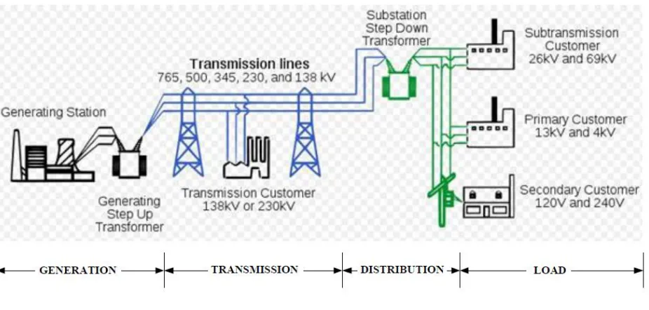
Distributed generation entered the electricity market solely because they provided solutions to overcome the shortfalls of the centralized generation paradigm. Figure 1.3 shows a 54-bus distributed energy system.
10
A „bus bar‟ is a high voltage or low voltage common collecting point for receiving and redistributing power. The utility sources are S1 & S2 and the distributed sources are DG1, DG2, DG3 & DG4 connected to the 110KV, 35KV, 35KV and 10KV voltage level busbars respectively as shown in figure above.
1.3.3. Technologies Used For Distributed Generation
According to the International Energy Agency, IEA (2002), the range of technologies for distributed generation can be categorized as follows [4]:
1. Reciprocating Engines:
This technology uses compressed air and fuel. The mixture is ignited by a spark to move a piston. The mechanical energy is then converted into electrical energy. Most reciprocating engines run either on fuel or natural gas with an increasing number of engines running on biogas produced from biomass and waste.
2. Gas Turbines:
They are widely used for electricity generation thanks to the regulatory incentives included to favour fuel diversification towards natural gas and their low emission levels. Gas turbines are widely used for cogeneration.
3. Micro turbines:
Micro turbines have the same characteristics as the gas turbines. But, the only differences that they have are lower capacities and higher operating speed.
4. Fuel Cells
11 5. Renewable Resources:
Renewal technologies have also been deployed to produce distributed energy. Renewal sources range from photovoltaic, wind energy, thermal energy etc. These sources qualify as distributed generation only if they meet the criteria of the definition which is not always the case.
1.3.4. Benefits of Distributed Generation
The distributed generation system has myriads of advantages over the centralized generation paradigm. The major benefits of decentralizing the electric power system are discussed below.
a. Reduction In T&D Losses
One of the key advantages of distributed energy is that it helps reduce transmission and distribution losses as distributed generators are not connected to the transmission grid. Some of them might even choose to operate as captive plant for a client with thus limited use of the distribution grid.
b. Reduction In T&D Distance
Since power is produced next to its point of use, transmission and distribution distance is greatly reduced. This explicitly affects the cost of installing transmission and distribution lines.
c. Quality of Power
Distributed generators can help improve the quality of services provided through voltage control (connecting a distributed generator to a low voltage network makes it possible to reduce the drop in voltage over the distance), providing additional peaking capacities.
d. Increase Power Capacity
12
e. Reliability
Unlike the centralized energy system, several electricity production facilities are connected to the distribution grid. Customers on the network no longer have to depend on a particular generating source. Hence, the pooling of resources to augment power supply ensures system reliability.
1.3.5. Challenges of Distributed Generation
a. Installation Issues
In the decentralized energy system, whenever a new generator is introduced reinforcement works will have to be undertaken. At times part or the whole system will have to be redesigned to cope with the changes. Besides, we have to incorporate control and protection software and hardware to coordinate with the distributed generators.
b. Voltage and Current Transients
Short term abnormal voltage or current oscillation may occur as distributed generators are switched on or off. The result of these oscillations can have a destabilizing effect on the network.
c. Reverse Power Flow
When the rotor speed of a distributed generator dips below the synchronous speed normally due to transient faults, the generator begins to behave like motor [37]. At this point, the machine loses its sense of purpose and instead of injecting power onto the grid; it turns into an „electrical vampire‟ and sucks power from the grid. This phenomenon seldom happens, but the possibility of its occurrence cannot be ruled out.
d. Harmonics
13
Non-linear loads such as rectifiers, computers, UPS, variable speed drive and industrial electronic equipment which contain power semiconductors such as Thyristor converters, inverters etc. are some of the sources of harmonics.
The above loads draw non-sinusoidal currents from the supply (generators) and lead to voltage distortions. This deviation from a perfect sine wave can be represented by harmonic components having a frequency that is an integral multiple of the fundamental frequency [8].
e. Formation of Islands
14 CHAPTER 2
ISLANDING CONCEPT
Electric power distribution systems have traditionally been designed assuming that the primary substation is the sole source of power. But, the advent of distributed generation has invalidated this assumption by placing power sources onto the distribution system. As a result, DG interconnection results in operating conditions which do not occur in a conventional system without generation directly connected at the distribution level. These operating situations present engineering challenges unique to distributed generation integration.
One of the new technical issues created by distributed generation interconnection is islanding. It could be intentional (when system is shut down for maintenance) or unintentional (when it happens as a result of an unanticipated fault). As per IEEE STD 1547-2003 [17], an island is a condition where a portion of a grid is energized solely by DGs while that portion of the grid is electrically separated from the rest of the power system. Therefore, we can say that intentional or unintentional island according to the above standard, is a planned or an unplanned island respectively. Figure 2.1 shows the pictorial illustration of islanding operation.
15
2.1. How Islands are Formed
The DG grid under normal operating conditions, maintain voltage and frequency within their standard permissible levels. Also, synchronism exists amongst all DGs on the distribution network and they operate together in unison with constant rotor speed.
When the system is driven into the unstable mode, DG protection system detects the fault and affected tie line is tripped. This action breaks the equilibrium that exists amongst the generators causing them to move out of step. The DGs swing haphazardly due to the deviations in their rotor angles. Interestingly, those generators with rotor angle deviations falling within a specific value will stick together in a group and operate as one entity supplying power to the local loads within its near vicinity. Two or more of such groups (coherent group) may result in a single or multiple swings.
The coherent groups of generators supplying power to local loads in their vicinity bring about an automatic partitioning of the power system into smaller sections called islands. The service in these islands is degraded and system components operate under extremely unacceptable conditions. This can be seen from the dynamic performance of the system at fault. In figures 2.2 and 2.3, a 15,549 bus system showing signs of islanding operations are illustrated [18].
16
2.2. Issues Related To Islanding
Islanding of distributed networks does present a number of safety, commercial, power quality, and system integrity problem. In summary, the major issues are [19]:
1. Islanding may create hazards for utility line workers or the public by causing a line to remain energized that may be assumed to be disconnected from all energy sources.
2. The distributed generators in the island could be damaged when the island is reconnected to the supply system. This is because the generators are likely to be out of synchronism with the system at the instant of reconnection. Such out-of-phase re-closing could result in large starter currents and damages to the generator shaft. It may also result in re-tripping in the supply system.
3. Unintentional islanding may interfere with the manual or automatic restoration of normal service for the neighboring customers.
4. Other major problems may be the isolated DG could cause abnormal voltage and frequency to the utility loads, which could be detrimental to the utility customers.
Due to these reasons, it is very important to detect the islanding quickly and accurately before the situation exacerbates.
2.3. Islanding Detection Techniques
Since islands pose a significant risk to safety and equipment, the ability to quickly detect and eliminate a power island is a critical requirement for both the DG owners and utilities. This is reflected in IEEE Std. 1547TM 2003 [20] and IEEE Std. 929-2000 [21] which specify that a DG should cease to energize the EPS within a specified time once an island occurs.
17
ISLAND DETECTION
REMOTE LOCAL
TRANSFER
TTRIP PLCC ACTIVE PASSIVE HYBRID
Fig. 2.4 Islanding detection techniques [19]
2.3.1. Remote Detection Technique
Most remote techniques for detection of islands are based on communication between the utility and the DGs. Usually remote detection schemes do not have a non-detection zone and are therefore very sound approaches for anti-islanding. However, remote techniques tend to be expensive to implement for small DG systems that do not otherwise require communication within the utility. Two popular detection methods are used under the remote and they are:
1. Transfer Trip (TT) Scheme:
18
2. Power Line Carrier Communication (PLCC) Scheme:
Here, a signal generator at the transmission system continuously sends a low-energy communication signal along the power line through a transmitter on the grid site [23]. The receiver, at the DG side can detect an islanding condition based on whether or not the receiver detects the presence of the PLCC signal. The use of PLCC for the detections of islanding does not degrade the quality of the generating power of the DG. It is also effective in multi-DG systems. Existing PLCC signals on the utility not originally intended for anti-islanding may be used to detect islands without interfering with their normal functions. Figure 2.5 shows a PLCC scheme.
Fig. 2.5 Power line carrier communication
2.3.2. Local Detection Technique
19
1. Passive Detection Techniques
Passive methods work on measuring system parameters such as variations in voltage, frequency, harmonic distortion etc. These parameters vary greatly when the system is islanded. Differentiation between an islanding and grid connected condition is based upon the threshold set for these parameters. Passive techniques are fast and they do not introduce disturbance in the system but they have a large non detectable zone (NDZ) where they fail to detect the islanding condition.
2. Active Detection Techniques
With active methods, islanding can be detected even under the perfect match of generation and load, which is not possible in case of the passive detection schemes. Active methods directly interact with the power system operation by introducing perturbations. The idea behind an active detection method is that this small perturbation will result in a significant change in system parameters when the DG is islanded, whereas the change will be negligible when the DG is connected to the grid.
3. Hybrid Detection Schemes
20 CHAPTER 3
LITERATURE REVIEW
The phenomenal growth in load demand in recent times has emerged as a potential challenge to the power system planners and operators. Fortunately, the advent of distributed generation system provided the solutions to the growing demand for electricity consumption. However, the installed DGs in the distribution system have introduced new issues in operational and planning levels. As discussed in previous chapters, uncontrolled islanding has become a major issue associated with distributed generation systems. The ravaging effects of this phenomena make it a huge concern to the utility industry.
In order to contain the impact of uncontrolled islanding when it happens without detection, research into finding the best candidates to counteract such undesirable conditions are far advanced. Some papers have studied controlled system islanding [11-18, 31-33], which means that the dispatch center actively trips some lines to split the power network into several maintainable islands according to asynchronous groups of generators and other requirements. System splitting has been widely acclaimed to be the last line of action to preventing blackout and maintain electricity supply for most customers, albeit the power network will be separated into asynchronous islands.
In islanding, it is not easy in real-time to determine the splitting strategy, namely which lines should be tripped (where to island), and when system splitting is imperative (when to island). However, though „where‟ and „when‟ to island are two mutually exclusive issues, the latter is beyond the scope of this thesis. References [34-36] have made some effort to solve these problems. Its main difficulties lie in the following aspects.
First, real-time decision-making requires extremely short strategy-search time, but the strategy space will explode exponentially with the increasing of size and complexity of the power network [35].
Secondly, the splitting strategy should satisfy necessary steady-state constraints, e.g. the following three constraints proposed in [35]:
21
b. generation-load imbalance in each island must be less than a prescribed limit,
c. all lines in each island must be loaded below their steady-state transmission capacity limits.
Therefore, identifying the appropriate cutsets to satisfy the above constraints is a strenuous challenge that requires exhaustive search technique. Many research efforts have consciously addressed these issues. The pre-determined boundary method had been used in the past. But this approach has become unfashionable because splitting the system along pre-defined cutsets had coherency issues [16].
In literatures [11-16], slow-coherency approach is used. Real-time computer search programs based on descriptive algorithms are developed to find the set of lines to trip. An analytical approach to automatically determine the islands from the identified slowly coherent groups of generators using an exhaustive cutset approach was developed in [12]. Paper [33] is also based on slow-coherency but further refined the islanding determination scheme using a max-flow min-cut, graph theoretic approach with capabilities to merge adjoining slowly coherent groups, or break coherent groups based on the location of the disturbance.
A new splitting scheme based on controlling group identification of generators other than slow- coherency is presented in [32]. A decision-making algorithm is used to find the optimal cutsets under different operational scenarios.
In [31], conjecture is used as a tool for cutset identification. The entire power system architecture together with its instability history is studied. The analysis is then used to surmise suitable splitting spots in future disturbance.
Reference [35] proposed a graph-model to represent a power network by which graph theory and Boolean algebra can be applied to represent and analyze splitting strategies. Based on ordered binary decision diagram (OBDD) representation [7], which is a high-efficiency technique for solving complicated Boolean algebra problems, [34] proposed a three-phase method to find the splitting strategies satisfying all constraints enumerated above in real-time.
22
frontiers until generation-load imbalance falls within the prescribed limit. The cutsets are identified from an adjacency matrix and the system is severed.
3.1. Controlled Islanding
Power system splitting is the final remedial action against inadvertent formation of islands following a severe disturbance. The main idea behind controlled islanding is to determine the proper splitting points for separating the entire power networks into smaller islands with their power mismatches falling within the permissible range. These islands are autonomous with their own power sources to sustain them. It is therefore the most desirable alternative to resolving uncontrolled system separations in power systems.
If a system disturbance causes zones A and B to separate from the system resulting in electrically unbalanced islands, the methodology for system splitting will have to address two major decision-making issues:
a) When to island b) Where to island
Many research contributions have addressed these pertinent issues [11]. In some literature, when to island starts right after the detection schemes have identified the uncontrolled islanding phenomena. However, where to island has been the spotlight of most research works.
Several methods have been proposed. Apart from the pre-determined boundaries approach, the rest make use of exhaustive searching strategies to locate the appropriate splitting spots that meet generation-load balance requirements. The most popular ones make use of genetic algorithms, artificial intelligence, conjecture and other heuristic algorithms.
23
3.2. Coherency Identification of Generators
The concept of coherency is very intuitive. Two machines are said to be coherent if after some disturbance, they present similar dynamical behavior, that is, their rotor angles and frequencies keep very similar along the system trajectories. Mathematically, one has:
Definition 3.2.1: Two machines are said to be ε-coherent or coherent with precision ε if
|δi (t)-δj (t)| < ε
Where δi and δj are respectively the rotor angles of machines i and j. As a limit case of the previous definition, one can say that two machines are perfectly coherent if ε=0 [6].
Coherency analysis in power systems is an important task which can supply very important information about the behavior of power systems. As, in general, the dimensions of the power system is very large, coherency analysis have been extensively used, in stability studies, to reduce the computational effort by aggregating coherent generators into a unique equivalent generator.
Under normal operating conditions, the rotor angles of all the generators swing together in the synchronous frame of reference prior to the occurrence of disturbance. This means the angular difference between any two generators is approximately constant over a period of time. The disturbance on the system causes drift in the rotor angle of some generators and hence these generators move away from the rest of the generators in the system and form different groups. The generators in each group are known as coherent generators. After the removal of the disturbance, the affected generators will again swing back to the rest of the generators. Formation of different coherent groups depends upon the nature of the disturbance occurring on the system.
24
With the exception of the classical approach, the rest are unsuitable for online applications. Therefore, it has given it the necessary impetus for extensive research. A number of contributions have appeared on the classical approach of identifying coherency in power systems with slow-coherency being the widely used method amongst the lots.
3.2.1. Slow Coherency Method
Slow coherency is increasingly becoming the most popular time-domain approach for identifying coherency amongst a pool of generators in power systems. This is because it provides a potential method for capturing the movement of generators between groups by analyzing their swing curves under disturbance. We define generators to be coherent if the waveforms of the rotor-angle trajectories are identical. In practice, however, they may be very close but not identical. Figure 3.1 shows the swing curves of some generators in a power system.
Fig. 3.1 Swing curve of a 56 bus system
25
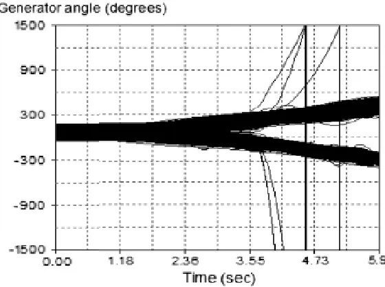
However, in very complex power systems (e.g. 25,000 buses), just analyzing the swing trajectories becomes a quixotic challenge. Fortunately, many power research labs have developed software packages based on slow coherency principle to identify coherency amongst a large number of generators in the power system network. One typical example is the „Dynamic Reduction Program‟, DYNRED, developed by the Electric Power Research Institute, EPRI, based in California, USA [24]. In [18], DYNRED was deployed into a 15,549 bus system in which 2385 generators were identified as belonging to two slowly coherent groups. There are 959 generators that belong to the North group and 1426 that belong to the south group. This is shown in figure 3.2 below.
Fig. 3.2 Swing trajectories of 15,549-bus system
3.3. Graph Theory
26
can be translated into a simple two-dimensional graph eliminating lots of redundant information [18]. The application of graph theory in power system islanding involves three operational parts:
a. Graph generation b. Graph simplification c. Graph partitioning
3.3.1. Graph Generation
The power grid is converted into a graph, G= (V, E). The inputs to the graph are nodes (v) and branches (e). In a real power system, nodes denote buses and branches represent transmission lined and at times transformers. Buses with generators are called generator nodes (vg) and those carrying loads are called load nodes (vl). So, for all vg VG and vl VL, we obtain the equation below.
V = VG VL
The terminologies used to better understand graph theory are given below.
a) Degree
The degree of a node is the number of branches connected to this node. It could be any non-negative integer. Zero degree means the node has no branch or connection.
b) Weight
The weight, w, is the active power flowing out of the node. It is positive if the node is converted from a generator bus and negative otherwise.
c) Domain
27
3.3.2. Graph Simplification
This operation is performed on the complex power system to trim or reduce its size to the desired form. However, simplifying the graph without losing too much useful information is also paramount. The following rules are employed in simplifying the graph.
a) Removal of degree one node
This rule could reduce both the size of nodes and branches of a graph.
Fig. 3.3 Removal of degree-one node
As shown above, node J can be removed from the graph without changing the total vertex weights by adjusting the weight of vertex I connected to them [18].
b) Removal of degree two node
For buses at which no loads and generators are connected, the power flow into the buses should equal the power flow out of the buses if power loss along the transmission lines is ignored. In figure 3.4 below, since no active power is injected at bus J, P1=P2=P. Hence, node J can be removed.
Fig. 3.4 Removal of degree-two node
c) Removal of Transformers
28
Figure 3.5 is a typical power system consisting of six buses and seven branches. After graph simplification, the 6-bus system is reduced to four buses and five branches. This is shown in figure 3.6. 600MW 55 53 95 94 253 250 44 42 200 196 238 235 300MW 235MW 200MW 1 3 4,6 5
Bus 1 Bus 2 Bus 3
Bus 4 Bus 5
Bus 6
250MW
Fig. 3.5 A 6-bus system Fig. 3.6 A 4-bus graph model
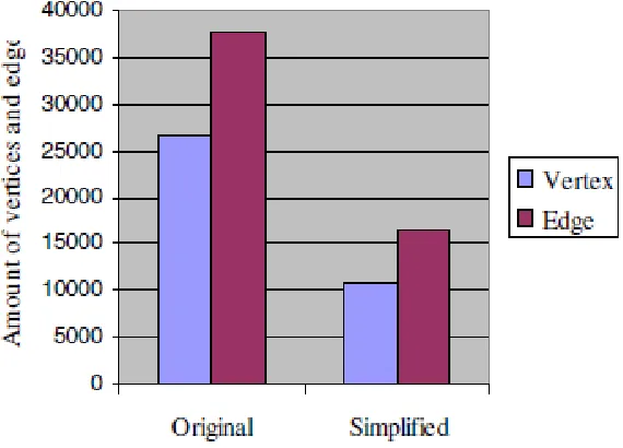
In [14], the power system comprises 37,839 edges and 26,552 vertices. After graph simplification, a significant amount of edges and vertices of the graph were eliminated and the computational cost for graph partitioning was reduced. This is shown in the figure below.
29
3.3.3. Graph Partitioning
Graph partitioning is the most crucial aspect of graph theory in power system islanding. Search algorithms are deployed to identify the appropriate splitting branches or cutsets after which the system is finally partitioned desirably to meet generation-load balance requirement. This is where our proposed partitioning algorithm is introduced.
3.4. Graph Searching Algorithms
Graph searching is a common approach to solving problems that are able to be modeled as a graph, G. since the power system can also be modeled as a graph through graph theory, knowledge of graph searching methods will be very useful. The most common ones are Dijkstra‟s algorithm, breadth-first-search (BFS), Depth-first-search (DFS), and Bellman-Ford-Moore‟s algorithm. In this section, the algorithm of Dijkstra‟s method will be discussed
3.4.1. Classical Dijkstra Algorithm
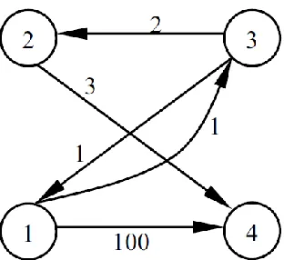
Dijkstra‟s algorithm, conceived by Dutch computer scientist Edsger Dijkstra in 1959, is a graph search algorithm that solves the single-source shortest path problem for a graph with nonnegative edge path costs, producing a shortest path tree. This algorithm is often used in routing, especially for transport, communication, routing protocols etc. For a given source vertex (node) in the graph, the algorithm finds the path with lowest cost (i.e. the shortest path) between that vertex and every other vertex. It can also be used for finding costs of paths from a single vertex to a single destination vertex by stopping the algorithm once the path to the destination vertex has been determined. For example, if the vertices of the graph represent cities and edge path costs represent driving distances between pairs of cities connected by a direct road, Dijkstra‟s algorithm can be used to find the shortest route between one city and all other cities.
30
Fig. 3.8 A directed graph
The results from Dijkstra are giveng below.
D[2, 3] = 0 D[3, 2] = 2 D[1, 3] = 1 D[1, 2] = 3 D[4, 2] = 0
31 CHAPTER 4
SOURCE NODE EXPANSION ALGORITHM (SNE)
Source Node Expansion (SNE) for slow coherency based islanding is a novel graph searching algorithm to determine optimal cutsets when splitting the power system into electrically balanced islands at post-fault. Canonically, when the power system is severely disturbed causing loss in synchronism, initial unbalanced islands are formed due to coherent grouping of generators.
The SNE initiates graph search for optimal cutsets from within each coherent group by starting source node expansion amongst individual generator nodes in each coherent group until cutsets are collectively found for the entire coherent group. This is achieved through a systematic frontier expansion across an Adjacency Matrix axis until generation-load balance is met. Once expansion terminates, for a particular coherent group, optimal cutsets can be found from matrix. This can be done by tracing up or down columns of locked load nodes during expansion. All entries, Aij=1, whose i remained unlocked during row expansion becomes the splitting spot. Hence, ei-j becomes the splitting edge or the cutset. Fig. 4.1 illustrates SNE.
32
4.1. How the Algorithm Works 4.1.1 Generator Grouping
Slow-coherency based generator grouping is the basis of Source Node Expansion Algorithm. A knowledge of the grouping information is imperative for setting the initial Islanding boundaries before graph search expansion is initiated from each coherent group. Slow coherency is discussed in detail in section 3.2.1 of Chapter 3.
4.1.2 Transport Network
After graph simplification and power flow tracing on the tie lines, a transport network is assembled, which is a directed graph, G = (V, E ) where V is the set of vertices and the edge set
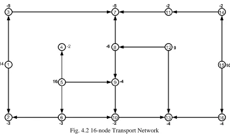
E, represents the total number of tie lines interconnecting the nodes. Fig. 4.2 shows a 16-node transport network with nodes 1, 5, 12 and 15 as generation or source nodes and the net power generation/consumption indicated next to each node; a positive number denotes total generated power of a source node and a negative value specifies the total power consumption of a load node. The units of these values are of no significance for the purpose of this algorithm.
33
Fig. 4.2 16-node Transport Network
TABLE 4.1
GROUPING DATA
GROUP NAME
GROUP MEMBER
TOTAL POWER (PU)
A 1,5 30
B 12 9
C 15 10
4.1.3 Dijkstra Implementation
After having transformed the post-disturbance power system into a transport network based on flow tracing, a modified Dijkstra algorithm is used. This algorithm solves the single-source, shortest-path problem for a graph where all edges have nonnegative weights [26].
34
destinations it visits based on the flow tracing pattern of the network.
The distance from one node to the other is translated into a cost, C. The source node is always used as the cost reference. A source node is called the root. In Fig. 4.3, the Dijkstra algorithm has been applied to source node 5. For this node, destinations 4, 6, and 9 are called parents and nodes 2 and 10 become are the children. Any node with an out-going degree of zero (no child) is called a leaf [27]. Destination 13 is a leaf. Node i is a brother of node j (i≠j) if nodes i and j have the same parent. Nodes 2 and 10 can be said to be brothers. Node i is an ancestor of node j (i ≠ j) if node i lies on the path from the root to node j. Nodes 6, 10 and 13 are the ancestors of node 5 figure below.
When we move from root node 5 to leaf node 13, a cost of C = 3 is assigned. This is done for all the nodes involved and the results are tabulated. This is shown in Table 4.2
35
TABLE 4.2
DIJKSTRA OUPUT
PATH TRAVEL
COST(C) A B
1 2 1
1 3 1
1 4 0
. . . . . .
5 9 1
5 10 2
5 11 0
. . .
16 14 0
16 15 0
16 16 0
4.1.4 Adjacency Matrix Formation
The output of the Dijkstra algorithm on the directed graph is now used to construct a matrix called the adjacency matrix. For a power system represented by a simplified graph containing N
36
Fig. 4.4. Adjacency matrix of the 16-node transport network
The rows of the adjacency matrix can be viewed as node power outflow and the columns as node power inflow. This will be evident when considering a node with power only flowing out (i.e. a source node), the column corresponding to this node will be all zeros.
4.1.5 Source Node Expansion Using Adjacency Matrix
The SNE algorithm considers the rows in the adjacency matrix corresponding to each source node. Before the start of expansion, all load nodes are considered to be unlocked. This means that they can be included or moved into any island provided that there is a tie-line connection. A node that is moved in one row will then be considered locked and cannot be moved in subsequent rows. This will eliminate thrashing, or repeated locking of the same node [28].
37
in the row representing a source node are regarded. First, any load node with direct connection to this source (i.e. any Aij= 1) is considered. If the source generates enough power to feed that load, its node will be moved into the island. This expansion and inclusion of loads will continue until the generation/load balance is reached or all the row elements with the value of 1 are moved. In the latter case, if the source can still provide more power, the same criteria is applied to all the nodes in its row with Aij= 2, then Aij = 3 and so on. The stopping criterion for the algorithm in each row is when the power balance condition is satisfied or all the nodes with Aij ≠ 0 are moved.
The next row to be studied is the next generator node in the same coherency group. The same expansion process is applied to this source followed by all the sources in this coherency group.
The next step is to establish the cutsets for this group of coherent generators. These can be determined by searching the columns related to all the locked nodes. Any Aij = 1 in the column representing an unlocked node will be one of the cutsets.
The final stopping criterion for the algorithm is when all the sources are expanded. This procedure can be illustrated using the adjacency matrix of Fig. 4.5 as an example:
38
The first row is considered corresponding to source node 1. At this node, SNE initiates at C = 1. The first entry, A12 representing a connection to load node 2 is moved and locked. This source node still has ample power generation so the next entry, A13 is visited and locked. Since the source node 1 has room to accommodate more loads and there are no more branches with C = 1 in this row, C = 2 is set. Expansion continues in a similar manner and A17 is locked which will satisfy generation-load mismatch for power balance requirement. The algorithm terminates for this row and C is set back to 1 for the next source node expansion, which is node 5 in the same coherency group as node 1. At C = 1, load nodes 4, 6 and 9 will be included and locked. Then at
C = 2, node 10 is moved (note that node 2 was already locked in the expansion of row 1 and hence not considered in this row). Since generator 5 can still accommodate more load, setting C
= 3, load 13 is included in this expansion, which will stop the algorithm for this row. At this point, by tracing the columns corresponding to the locked nodes 2, 3, 4, 6, 7, 9, 10 and 13, searching for all the 1‟s associated with an unlocked node, the cutting edges of , e8-7, e8-9, e12-13 and e16-13are determined. The algorithm continues for all the source nodes and the final cutset is found to be Efinal = {e8-7, e8-9, e11-7, e12-13, e16-13}. The islands now can be formed as shown in Fig. 4.6. It is clear that generation-load mismatch is satisfied in each island.
39
This algorithm is also able to reduce the number of loads that need to be shed in order to provide system stability and maintain dynamic performance.
4.1.6 Final Separation
The final system splitting is shown in Fig. 4.7. Table 4.3 shows that acceptable power mismatch exists amongst the three balanced islands.
Fig. 4.7 Balanced Islands
TABLE 4.3
GENERATION-LOAD MISMATCH DATA
ISLAND TOTAL GENERATION
(PU)
TOTAL LOAD (PU)
A 30 28
B 9 6
C 10 8
40 CHAPTER 5
CASE STUDY
This chapter covers the testing of the algorithm in a simulated environment. A 3 phase-to-ground fault is considered. A 14-bus system and a 37-bus system are tested to verify the SNE algorithm. The PowerWorld Simulator software is used to display the implications of the SNE algorithm.
5.1. The 14-Bus System
5.1.1. System Design
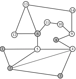
Figure 5.1 shows a 14-bus system with 5 generators and 10 loads. This system can be an
example of a distribution network with several DG sources with varying production capabilities
Fig. 5.1 14-Bus system
5.1.2. The 14-Bus Graph Model
41
1
8
9
10
11
13
2
6
3
4
5
12
14
Fig. 5.2 Simplified graph of 14-Bus System
TABLE 5.1
LOAD INFORMATION
BUS NO. 2 3 4 5 6 7
POWER 21.7 94.2 47.8 7.6 0 0
BUS NO. 9 10 11 12 13 14
POWER 29.5 9 3.5 6.1 13.5 14.5
TABLE 5.2
GENERATOR INFORMATION
BUS NO. 1 2 3 6 8
POWER 232.4 42.4 23.4 12.2 17.4
5.1.3. Fault Analysis a. Contingency 1
42
synchronous speed and Fig. 5.10 displays the bus voltage magnitudes. Significant voltage oscillation as well as system instability is observed. It is evident that the dynamic performance of the system is completely unacceptable and a complete halt of operation is the only way to deal with this situation.
5.1.4. Simulation Results a. 14-Bus Swing Curve
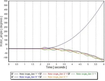
Fig. 5.3 shows the generator rotor-angle trajectories of the 14-bus system. From the graph, two coherent groups could be identified. Generator node 6 exists on its own as a coherent group and the rest (generator nodes 1, 2, 3 and 8) belong one coherent group.
Fig. 5.3 Generator angles after contingency
43
The graphs below shows the detailed rotor-angle response curves of all the five generators on the fourteen-bus system.
Fig. 5.4 Generator 1 rotor angle Fig. 5.5 Generator 2 rotor angle
Fig. 5.6 Generator 3 rotor angle Fig. 5.7 Generator 6 rotor angle
44
b. Rotor Speed Deviation
Figure 5.10 is the generator rotor deviations from synchronous speed. Speed deviation is constant before contingency. Unstable speed deviations are observed after contingency.
Fig. 5.9 Generator speed deviations after contingency
c. Bus Voltages
45
Fig. 5.10 Bus voltage magnitudes after contingency
5.1.5. Cutset Search a. Transport Network
A MATLAB program in Appendix A.1 is used to convert the graph in Fig. 5.2 into a transport network. This is displayed in Fig. 5.11.
46
b. Dijkstra‟s Algorithm
The transport network is used as input to Dijkstra algorithm to compute the cost, C. Table 4.4 shows the output results from Dijkstra algorithm.
TABLE 5.3
DIJKSTRA RESULTS
c. Adjacency Matrix Formation
The data shown in Table 5.3 is used to form the Adjacency Matrix to deduce the optimal cutsets. The final Adjacent Matrix formed is displayed in Table 5.4.
PATH TRAVEL COST
A B
1 2 1
1 3 2
1 4 3
. . . . . . . . .
6 10 0
6 11 1
6 12 1
. . . . . . . . .
14 12 2
14 13 1
47 TABLE 5.4 ADJACENCY MATRIX
The optimal splitting branches were identified after row expansions. The red-circled entries denote the cutsets. Therefore, Efinal = {e5-6, e6-13, e13-16, e7-8 , e7-11, e12-13, e8-9}.
5.1.6. Final Separation
The figures below illustrate the formation of two electrically balanced islands after SNE algorithm is implemented.
48
1
2
3 4
5 6
9 13 11
12
10 14
8
Island A
Island B
Fig. 5.14 Balanced islands
5.1.7. Bus Voltage Comparison
Table 5.5, shows the bus-to-bus voltage comparisons for scenarios a and b.
TABLE 5.5
BUS VOLTAGES
a. Bus Voltage after contingency b. Bus Voltage after Islanding
49
Bus 2 voltage after contingency Bus 2 voltage after Islanding
Bus 3 voltage after contingency Bus 3 voltage after islanding
50
Bus 8 voltage after contingency Bus 8 voltage after islanding
51 5.2.The37-Bus System
5.2.1. System Design
This case models a 37-bus system with 8 generators and 24 loads. It also contains three different voltage levels (345kV, 138kV, and 69kV) and 57 transmission lines. Fig. 5.15 shows the single line diagram of the 37-bus system.
52
5.2.2. The 37-Bus Graph Model
Fig. 5.16 displays the simplified graph model of the 37-bus system. After graph simplification, system complexity is reduced. The branches are downsized to 46. Table 5.6 contains bus names and their corresponding bus numbers information.
1 2 4 7 3 5 6 14 15 9 10 8 16 12 17 11 13 18 20 21 19 24 23 22 25 26 27 28 29 30 31 32 33
34 35 36
37
![Fig. 1.3 One line diagram of a distributed generation system [5]](https://thumb-us.123doks.com/thumbv2/123dok_us/1443983.1176913/20.612.70.550.366.669/fig-one-line-diagram-of-distributed-generation-system.webp)