Scholarship at UWindsor
Scholarship at UWindsor
Electronic Theses and Dissertations Theses, Dissertations, and Major Papers
Summer 7-16-2019
Development of dynamic model and control techniques for
Development of dynamic model and control techniques for
microelectromechanical gyroscopes
microelectromechanical gyroscopes
Md imrul Kaes University of Windsor
Follow this and additional works at: https://scholar.uwindsor.ca/etd
Recommended Citation Recommended Citation
Kaes, Md imrul, "Development of dynamic model and control techniques for microelectromechanical gyroscopes" (2019). Electronic Theses and Dissertations. 7769.
https://scholar.uwindsor.ca/etd/7769
This online database contains the full-text of PhD dissertations and Masters’ theses of University of Windsor students from 1954 forward. These documents are made available for personal study and research purposes only, in accordance with the Canadian Copyright Act and the Creative Commons license—CC BY-NC-ND (Attribution, Non-Commercial, No Derivative Works). Under this license, works must always be attributed to the copyright holder (original author), cannot be used for any commercial purposes, and may not be altered. Any other use would require the permission of the copyright holder. Students may inquire about withdrawing their dissertation and/or thesis from this database. For additional inquiries, please contact the repository administrator via email
gyroscopes
By
Md. Imrul Kaes
A Thesis
Submitted to the Faculty of Graduate Studies
through the Department of Mechanical, Automotive & Materials Engineering
in Partial Fulfillment of the Requirements
for the Degree of Master of Applied Science
at the University of Windsor.
Windsor, Ontario, Canada
gyroscopes
by
Md. Imrul Kaes
APPROVED BY:
______________________________________________ G. Kabir
Department of Mechanical, Automotive & Materials Engineering
______________________________________________ N. Zamani
Department of Mechanical, Automotive & Materials Engineering
______________________________________________ D. Ting, Co-Advisor
Department of Mechanical, Automotive & Materials Engineering
______________________________________________ J. Ahamed, Advisor
Department of Mechanical, Automotive & Materials Engineering
DECLARATION OF CO-AUTHORSHIP / PREVIOUS PUBLICATION
I. Co-Authorship
I hereby declare that this thesis incorporates material thatis result of joint research, as follows:
Chapter 4 and 5 of the thesis were co-authored with J. Ahamed. In all cases, primary contributions, experimental designs, data analysis, interpretation, and writing were performed by me and J. Ahamed contributed to the key ideas; D. Ting provided feedback on refinement of ideas and editing of the manuscript.
I am aware of the University of Windsor Senate Policy on Authorship and I certify that I have properly acknowledged the contribution of other researchers to my thesis, and have obtained written permission from each of the co-author(s) to include the above material(s) in my thesis.
I certify that, with the above qualification, this thesis, and the research to which it refers, is the product of my own work.
II. Previous Publication
Thesis Chapter Publication title/full citation Publication status
Chapter [4] Md. Imrul Kaes, David S-K Ting, Mohammed Jalal Ahamed “ Modeling of Structural and Environmental Effects on Microelectromechanical (MEMS) Vibratory Gyroscopes,” Canadian Society for Mechanical Engineers Conference 2018.
Published: Conference: 2018 Canadian Society for Mechanical Engineering (CSME) International Congress
I certify that I have obtained a written permission from the copyright owner(s) to include the above published material(s) in my thesis. I certify that the above material describes work completed during my registration as a graduate student at the University of Windsor.
III. General
I declare that, to the best of my knowledge, my thesis does not infringe upon anyone’s copyright nor violate any proprietary rights and that any ideas, techniques, quotations, or any other material from the work of other people included in my thesis, published or otherwise, are fully acknowledged in accordance with the standard referencing practices. Furthermore, to the extent that I have included copyrighted material that surpasses the bounds of fair dealing within the meaning of the Canada Copyright Act, I certify that I have obtained a written permission from the copyright owner(s) to include such material(s) in my thesis.
ABSTRACT
In this thesis we investigate the effects of stiffness, damping and temperature on
the performance of a MEMS vibratory gyroscope. The stiffness and damping parameters
are chosen because they can be appropriately designed to synchronize the drive and sense
mode resonance to enhance the sensitivity and stability of MEMS gyroscope. Our results
show that increasing the drive axis stiffness from its tuned value by 50%, reduces the sense
mode magnitude by ~27% and augments the resonance frequency by ~21%. The stiffness
and damping are mildly sensitive to typical variations in operating temperature. The
stiffness decreases by 0.30%, while the damping increases by 3.81% from their initial
values, when the temperature is raised from -40 to 60C. Doubling the drive mode damping
from its tuned value reduces the oscillation magnitude by 10%, but ~0.20% change in the
resonance frequency. The predicted effects of stiffness, damping and temperature can be
DEDICATION
This work is dedicated to my maker whom by grace, through faith, redeemed my soul
ACKNOWLEDGEMENTS
I would like to acknowledge the leadership, wisdom, and support provided by my
primary advisor, J. Ahamed, and co-advisor, David S-K. Ting. The guidance and patience
they have given me has been essential throughout the past two years and has helped me to
grow. I would also like to thank N. Zamani and G. Kabir for their contributions in providing
their time and knowledge to keep me on track in my master’s project. I would like to thank
the Natural Sciences and Engineering Research Council of Canada (NSERC) and
TABLE OF CONTENTS
DECLARATION OF CO-AUTHORSHIP / PREVIOUS PUBLICATION ... iii
ABSTRACT ...v
DEDICATION... vi
ACKNOWLEDGEMENTS ... vii
LIST OF FIGURES ...x
LIST OF ABBREVIATIONS ... xiii
NOMENCLATURE ...xv
CHAPTER 1: INTRODUCTION ...1
1.1 Applications of MEMS Gyroscopes ...1
1.2 Types of Gyroscopes ...3
1.3 Gyroscope Performance Specifications ...7
1.4 Vibratory Gyroscope Principle ...8
1.5 Literature review: ...9
CHAPTER 2: OBJECTIVE & METHODOLOGY ...11
CHAPTER 3: MODELING GYROSCOPE DYNAMICS ...13
CHAPTER 4: MODEL RESULTS ...18
4.1 Effect of stiffness (Drive Mode) on resonance frequency ...19
4.2 Effect of stiffness (Sense Mode) on resonance frequency ...21
4.3 Effect of stiffness (both Drive Mode and Sense Mode) on resonance frequency ...21
4.4 Effect of damping (Drive Mode) on resonance frequency ...23
4.5 Effect of temperature variation on stiffness and damping ...24
4.6 Effect of temperature variation on stiffness coefficient ...25
4.8 Effect of mass variation on resonance frequency ...28
CHAPTER 5: CONTROLLER ...30
CHAPTER 6: CONCLUSION ...47
CHAPTER 7: FUTURE WORK ...49
7.1 Why Fuzzy Logic Controller ...49
7.2 How does fuzzy controller work? ...49
REFERENCE ...53
LIST OF FIGURES
Figure 1: Mechanical Gyroscope ... 4
Figure 2: Optical gyroscope ... 5
Figure 3: MEMS Vibratory gyroscope ... 6
Figure 4: MEMS Gyroscope Developed at Micro Nano Mechatronics Lab at University of Windsor ……….6
Figure 5: The vibratory gyroscope principle (a) (b) (c) ... 9
Figure 6: SIMULINK model of gyroscope ... 16
Figure 7: Frequency-Response Curve ... 18
Figure 8: Effect of drive mode stiffness on output sense (sense mode stiffness is constant) ... 20
Figure 9: Effect of drive mode stiffness on resonance frequency and its magnitude ... 20
Figure 10: Effect of sense mode stiffness on resonance frequency ... 21
Figure 11: Combined effect of drive mode stiffness and sense mode stiffness on magnitude ... 22
Figure 12: Effect of drive mode stiffness and sense mode stiffness on output sense ... 23
Figure 13: Effect of drive mode damping on resonance frequency ... 24
Figure 14: Relationship between temperature and stiffness ... 26
Figure 15: Relationship between stiffness and magnitude when temperature changes .... 26
Figure 16: Relationship between temperature and damping ... 27
Figure 17: Relationship between damping and magnitude when temperature changes ... 27
Figure 19: Effect of angular rate variation on output signal ... 29
Figure 20: Input Signal (Drive Direction) ... 30
Figure 21: Output Signal (Sense Direction) ... 31
Figure 22: Hypothetical Input Signal ... 31
Figure 23: Hypothetical Expected Output Signal ... 31
Figure 24: Hypothetical Actual Output Signal ... 32
Figure 25: Hypothetical Repaired Signal by using Controller... 32
Figure 26: Noise without controller at 1 rad/s angular rate ... 34
Figure 27: Step responses for different P, I, D, N values ... 40
Figure 28: Signal characteristics for different P, I, D, N values ... 41
Figure 29: Slew rate ... 42
Figure 30: Noise reduced after using after continuous PID controller at 1 rad/s angular rate... 42
Figure 31: Noise reduced after using after discrete PID controller at 1 rad/s angular rate43 Figure 32: Unit step response without controller ... 44
Figure 33: Unit step response with PID controller ... 45
Figure 34: Comparison of signal characteristics between no controller and PID controller ... 46
LIST OF TABLES
Table 1: Typical performance grades for gyroscopes ... 8
Table 2: Signal characteristics for different P, I, D, N values ... 35
Table 3: Continuous PID controller tuned parameters ... 43
Table 4: Discrete PID controller tuned parameters ... 44
Table 5: Comparison between without controller and PID controller at transient zone ... 45
Table 6: Fuzzy Set Operations ... 51
Table 7: Accumulation Methods ... 51
LIST OF ABBREVIATIONS
2-DOF Two Degrees-of-Freedom
ADI Analog Devices Inc.
ASIC Application-specific integrated circuit
CMOS Complementary Metal- Oxide Semiconductor
CVD Chemical Vapor Deposition
DETF Double-Ended Tuning Forks
DRIE Deep Reactive Ion Etching
ESD Electrostatic discharge
HMDS Hexamethyldisilazane
IC Integrated Circuit
ICP Inductively Coupled Plasma
JPL Jet Propulsion Laboratory
LIGA Lithography Galvanoformung Abformung
LPCVD Low-Pressure Chemical Vapor Deposition
MEMS Microelectromechanical Systems (MEMS)
PECVD Plasma Enhanced Chemical Vapor Deposition
PSG Phosphosilicate Glass
PVD Physical Vapor Deposition
RIE Reactive Ion Etching
SOG Silicon-on-Glass
SOI Silicon-on-Insulator
TMAH Tetramethylammonium hydroxide
UV Ultra Violet
NOMENCLATURE
d Demping coefficient at reference temperature of 300 K
dxx Damping coefficient along the drive-axis
dxy Damping error due to manufacturing imperfection
dyy Damping coefficient along the sense-axis
K0 Stiffness coefficient at reference temperature 300 K
kxx Spring stiffness along the drive-axis
kxy Stiffness error due to manufacturing imperfection
kyy Spring stiffness along the sense-axis
m Proof Mass
CHAPTER 1: INTRODUCTION
A gyroscope is a device mounted on a frame used for measuring or maintaining
orientation and angular velocity if the frame is rotating. It is a sensing device that measures
the angular rate of an object [1]. A conventional spinning wheel gyroscope is a spinning
top combined with a pair of gimbals. The first known device similar to a gyroscope was
introduced by John Serson in 1743 [2]. Johann Bohnenberger of Germany, first used a
device like an actual gyroscope in 1816 who first wrote about it in 1817 [3]. Foucault gave
this device a modern name (Greek skopeein, to see) the Earth's rotation (Greek gyros, circle
or rotation) [4]. German inventor Hermann Anschütz-Kaempfe patented the first functional
gyrocompass in 1904 [5]. At the beginning of 20th century other devices started to use
gyroscopes [6]. Military use of gyroscope has been started widely after the miniaturization
technique has been invented [7].
1.1 Applications of MEMS Gyroscopes
Because of wide availability of motion, vibration and shocks, there is almost no
place where inertial sensors are not found. Though the initial interest on gyroscope started
with navigation, telescope, imaging system and antennas, it is has now spread everywhere
including automotive industry because of its low cost, high reliability and possibility of
mass production [8].
Navigation: Inertial navigation sensors (INS) now a days are used to figure out the
systems for non-holonomic constraints and using odometer measurements. Pedestrian
navigation systems using biomechanics help many disable people walking. Inertial sensors
are widely used for identifying the occurrence of steps which helps estimating the distance
and direction in which the steps were taken.
Automotive: Recent cars use MEMS accelerometers for airbag deployment systems
which is further used for detecting a rapid negative acceleration of the vehicle, finding out
if a collision is happened, and calculating the severity of the collision. MEMS gyros and
accelerometers are also used in electronic stability control systems to keep the car towards
its intended direction. MEMS gyroscope is also used in conditions that cause discomfort
for drivers and passengers, harshness and monitoring of noise.
Industrial: In industry, accelerometer has wide application specially in monitoring
vibration. Bearing fault in rotating equipment such as turbines, pumps, fans, rollers,
compressors, and cooling towers, gear failure, reduce downtime are some major
applications of MEMS gyroscope.
Consumer Products: The miniaturization of accelerometers and gyroscopes
revolutionized the industry of game controllers, mobile phones, cameras, and other
personal electronic devices. Other popular applications are sport and healthy lifestyle,
gesture recognition, orientation sensing, motion input, image stabilization and fall
Inertial sensor embedded cameras are used for image stabilization. Fall detection feature
now has become common for many consumer products by the virtue of accelerometer.
Sport: Today’s pedometer is a gift of modern accelerometer which is the simplest form
of step counter. Inertial sensors contributed a lot to the technology of motion analysis
specially javelin, ski jumping and figure skating. Now we can easily detect not only human
movement but also the movement of different parts of the body and these data are used in
medical and virtual environments.
1.2 Types of Gyroscopes
Several kinds of gyroscopes are available in the market. Most common ones are
mechanical gyroscope, optical gyroscope and microelectromechanical gyroscope.
Mechanical Gyroscopes
In this kind of gyroscope, a mass called spinning mass, spins around its axis. The
special feature of it is that when the mass spins it tries to stay parallel to itself and to oppose
any attempt to change its orientation. Léon Foucault discovered this mechanism.
Precession and nutation are few of the many physical phenomena that mechanical
gyroscope shows. Figure 1 shows typical mechanical gyroscope. In mechanical gyroscope,
proof mass tries to remain in its angular position and when an external torque is introduced,
Figure 1: Mechanical Gyroscope
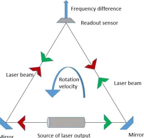
Optical Gyroscopes
The basic feature of optical gyroscope is the laser cavity in the light path which
augment the Signac effect. The basic principle of the optical gyroscope shows in Figure 2.
An active source of laser output is used in a confined cavity. The cavity has reflecting
mirrors. A pair of laser beam is directed at the same time in two opposite directions. When
and therefore, frequency difference occurs. Time varying phase shift appears due to this
frequency difference and number of beat period can be calculated from it. From this beat
period, angular increment can be easily found out.
Figure 2: Optical gyroscope
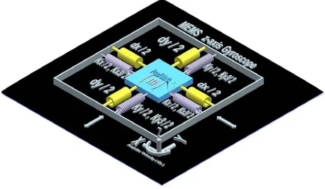
Microelectromechanical (MEMS) gyroscopes
MEMS gyroscopes utilize vibrating structure as a sensing element for identifying
the angular velocity. They consist of bearings. When the proof mass vibrates and given a
rotation, a force named Coriolis introduced which transfer energy between two vibration
modes. The Coriolis force is proportional to the angular velocity. Figure 3 shows typical
Figure 4: MEMS Gyroscope Developed at Micro Nano Mechatronics Lab at
University of Windsor
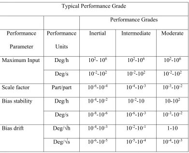
1.3 Gyroscope Performance Specifications
The performance specifications of gyroscope are mentioned in the IEEE Standard
Specification Format Guide and Test Procedure for Coriolis Vibratory Gyros [10]. The
following is a summary of important specifications [11].
Scale factor: It is the ratio of output change in respect to input change which is
measured in mV/°/second.
Nonlinearity: It is the shift from the line which represents the relationship between inputs
and outputs.
Scale factor temperature and acceleration sensitivity: It is the drift in scale factor which
occurs due to a change in steady state operating temperature and a constant acceleration.
Bias: It is the mean over a specific time of gyroscope output which is quantified in specific
operating conditions. Bias is measured in °/sec or °/hr.
Environmentally sensitive drift rate: It depends on environmental parameters which
includes temperature hysteresis, acceleration sensitivity, temperature sensitivity,
temperature gradient sensitivity, vibration sensitivity etc.
Shock Resistance: It is the maximum shock that the operating or non-operating equipment
can stand before failure [12]. This shock resistance are determined during testing and
Table 1: Typical performance grades for gyroscopes
Typical Performance Grade
Performance Grades
Performance
Parameter
Performance
Units
Inertial Intermediate Moderate
Maximum Input Deg/h 102- 106 102-106 102-106
Deg/s 10-2-102 10-2-102 10-2-102
Scale factor Part/part 10-6-10-4 10-4-10-3 10-3-10-2
Bias stability Deg/h 10-4-10-2 10-2-10 10-102
Deg/s 10-8-10-6 10-6-10-3 10-3-10-2
Bias drift Deg/√h 10-4-10-3 10-2-10-1 1-10
Deg/√s 10-6-10-5 10-5-10-4 10-4-10-3
1.4 Vibratory Gyroscope Principle
In vibratory gyroscope the proof mass can freely vibrate in the drive and the sense
directions. The proof-mass is accelerated in the drive direction by a sinusoidal force
introduced from outside. When the gyroscope is given an angular rotation, a sinusoidal
Coriolis force at the frequency of drive mode oscillation is introduced in the sense
direction. The Coriolis force makes the proof-mass to oscillate in the sense direction and
(a) (b) (c)
Figure 5: The vibratory gyroscope principle (a) (b) (c)
1.5 Literature review:
Microelectromechanical systems (MEMS) inertial sensors like accelerometers and
gyroscopes are the most popular MEMS technology till now. With the rapid development
of fabrication technology, the cost and size of MEMS are decreasing and the power is
increasing which is augmenting new uses in automotive, aerospace, biomedical and
consumer electronics. MEMS vibratory gyroscopes find its wide application in detecting
the angular rate of an object in respect of a reference frame [14] [15] [16] [17]. A proof
mass is used to calculate the angular rotation [2]. The Coriolis Effect plays a key role for
measuring this rate of rotation [18]. Because external disturbances, it becomes almost
impossible to get the accurate value of resonant frequencies which reduces the performance
of gyroscope. Therefore, proper design and optimization of influencing parameters are
parameter modeling can be helpful to design a robust system [4]. These methods are robust,
flexible and accurate and can be used with controllers and electronics for better result [5]
[19]. In MEMS gyroscopes, manufacturing defects always exist which adversely affect the
performance. Robust and efficient controllers are necessary for the compensation [20].
However, quantitative measurement of the individual and combined influence of
stiffness, damping and temperature on MEMS gyroscope have not been found in the
literature. In this thesis, a lumped-parameter model for predicting the gyroscope
performance with the influence of various system parameters such as stiffness, damping
and environmental condition (temperature) have been analyzed. The results can be utilized
CHAPTER 2: OBJECTIVE & METHODOLOGY
This section includes the description of the specific objectives and methods for
(1) The development of a lumped parameter model to capture MEMS vibratory
gyroscope dynamics.
(2) The investigation of the effects of temperature, stiffness and damping on the
performance of a MEMS vibratory gyroscope. For example, for stiffness 80.98 N/m,
damping coefficient 71.62 N s/m and at 300 K temperature resonance frequency is
found at 19.4 kHz with magnitude 5.40 dB and amplitude 0.025 μm. Our
investigation will focus on what percentage of amplitude, magnitude and resonance
frequency change when the values of stiffness coefficient, damping coefficient and
temperature are varied with in certain range like stiffness and damping coefficient
from half to double, temperature from 270 K to 330 K.
(3) The augmentation of the gyro performance (reduce noise) using advance
controller.
There are three primary steps which have been followed in this study:
(1) To develop a model relating to gyroscope vibrational characteristics with
temperature, stiffness, proof mass, angular rate and damping.
(2) To perform simulation and experiment to evaluate the effects of temperature,
stiffness and damping on gyro performance.
According to the equation of motion, the dynamics of gyroscope have been
developed. We assumed that the behavior of the spring is linear. Frequency response curve
has been used to compare the effects of varying stiffness, damping and temperature on gyro
performance. Frequency response curve shows the comparison between the output and
input as a function of frequency. Magnitude is the logarithmic ratio of output and input.
The decibel is used for measuring magnitude. If output amplitude is smaller than input,
magnitude becomes negative. MATLAB Simulink [21] is used for simulation and
computation. As the performance of the MEMS gyroscope is often deteriorated by the
effects of time-varying parameters, quadrature errors and external disturbances, we need a
controller. After considering advantages and limitations of different controllers, we select
CHAPTER 3: MODELING GYROSCOPE DYNAMICS
Typical MEMS vibratory gyroscope consists of a proof mass, spring suspensions,
electrostatic actuations and sensing mechanisms. These mechanical arrangements can be
considered as a mass, spring, and damper system. In this thesis, only linear vibratory
gyroscopes are considered. Figure 3 shows a simplified model of a MEMS gyroscope
having two degrees of freedom. Assuming that the proof mass can only move along the x
and y plane by making the spring stiffness in the z direction. Considering the angular rate
almost constant, the equation of motion of a gyroscope is simplified as follows.
mx+dxx x + (kxx – m (Ωy2+ Ωz2)) x + m ΩyΩx y = ux + 2m Ωz y (1)
my+dyy x + (kyy – m (Ωx2+ Ωz2)) y + m ΩyΩxx = uy - 2m Ωz x (2)
Here dxy, kxy are cross damping and cross spring coefficients, Ω is the angular
velocity, ux, u y are external forces. 2m Ωz x and 2m Ωz y are Coriolis forces Equation 1
and Equation 2. According to the assumption only Ωz, causes a dynamic coupling and due
to this Ωx2 ≈ Ωy2 ≈ Ωx2Ωy2 ≈ 0 has been considered. As manufacturing imperfection will
be always there Equation 1 and Equation 2 are modified as Equation 3 and Equation 4 as
follows [22]:
Equation 3 shows the force balance between external force, Coriolis force and acceleration
force, stiffness force, cross stiffness force, cross damping force to the drive direction.
my+dyyy+ kyy y +kxy x + dxyx= uy- 2m Ωzx (4)
Equation 4 shows the force balance between external force, Coriolis force and acceleration
force, damping force, cross stiffness force, cross damping force to the sense direction.
Manufacturing imperfections are represented with spring and damping terms, kxy
and dxy. The drive and sense mode spring and damping are represented by kxx, kyy, dxx and
dyy are deterministic [23]. To make the numerical simulation easy, scaling of the equations
have been performed. The realization of dimensional control is done by multiplying the
dimensionalizing parameters with the scaled terms. q0 and w0, are the length and natural
resonance frequency respectively and the scaling of Equation 5 and Equation 6 can be done
as follows:
x x+dxyy w x +wxy y = ux+2 Ωz y (5)
y y+dxyx w y +wxy x = uy-2 Ωz x (6)
Where Qx and Qy are respectively the drive and sense quality factors,
wx= , wy= , wxy= , dxy ← , Ωz←Ω , ux ← , , uy ←
We can describe mathematically the governing equations for typical mode of
x =X0 sin (wxt) (7)
y + y w y= uy - wxy x – (dxy +2 Ωz)x (8)
The negative impact of the cross damping dxy on gyroscope performance has not
been considered by many researchers so far. However, its effect should not be
underestimated [24]. In reality it is not easy to identify and cover up for all the
manufacturing imperfections. One way to get these manufacturing imperfections
compensated by creating richer gyroscope dynamics.
Simulation has been done to observe the influence of stiffness, damping and
temperature on gyroscope performance to minimize time and cost of expensive trial and
error with the actual fabrication cycle [12]. The SIMULINK model (Figure 6) has been
developed from the Equation 3 and Equation 4. The following parameters have been used
for simulation - proof mass, m = 0.57e -8 kg, damping coefficient along the drive-axis, d xx
= 0.429e-6 N s/m, damping error due to manufacturing imperfection, d
xy = 0.0429e−6 N s/m,
damping coefficient along the sense-axis, dyy = 0.687e−6 N s/m, spring stiffness along the
drive-axis, kxx= 80.98 N/m, stiffness error due to manufacturing imperfection, kxy = 5 N/m,
spring stiffness along the sense-axis, kyy = 71.62 N/m, angular velocity, Ωz= 5 rad/s are
Figure 6: SIMULINK model of gyroscope
In this SIMULINK model we apply a sinusoidal voltage as an input as an
external force ux and sense the displacement in both in drive (x) and sense (y) directions.
As it is a second order equation, we integrate acceleration and velocity to get the
displacements. For stiffness, damping, cross stiffness, cross damping, proof mass, angular
velocity, tuned values have been used from the literature. To balance, the forces are
connected to nodes with appropriate signs. Directions are shown with arrows.
Multiplications are shown with triangles with values inside. Here “Sum 1 node” is actually
the other hand “Sum 2 node” is constructing Equation 4 which is balancing my, dyy y, kyy
y, kxy x, dxy x, uy, 2m Ωz x. For integration we use “Integrator” and to watch the output we
added “Scope” in the model. We get the Bode-Plot by setting the frequency range from 1
kHz to 100 kHz with linearly spaced 10,000 frequencies. To smooth the curve 100 moving
CHAPTER 4: MODEL RESULTS
Parameters have been varied on the model in Matlab SIMULINK, developed
in chapter 2. The parameters varied are mass, angular rate, spring stiffness, damping
coefficient and temperature which influence the output performance of gyroscope. Thus,
the objective of the simulation is to quantify the effects of these parameters. These
parameters are very vital for equipment where the resonance frequency is the principal
factor in determining the gyro performance [25].
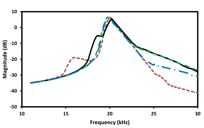
After sweeping the simulation with the frequency range of 1 kHz to 60 kHz ( Figure
7), the resonance frequency is found at around 19.4 kHz. So, for better focusing, the
frequency range is restricted from 10 kHz - 30 kHz for other comparisons.
Figure 7: Frequency-Response Curve ‐50
‐40 ‐30 ‐20 ‐10 0 10
0 15 30 45 60
Magnitude
(dB)
The spring stiffness and damping coefficient are varied from half to double of their
nominal values. The temperature is varied from -400 C to 600 C to observe the temperature
effect on stiffness, damping coefficient and on sensing magnitude. For the simulation
model, the nominal values for the proof mass, stiffness, and damping are extracted from
the literature reported in [26].
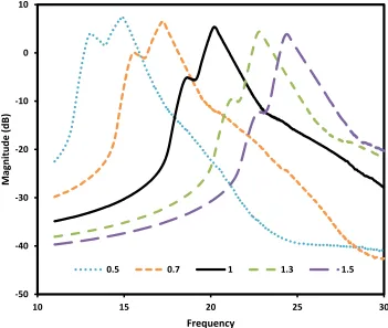
4.1 Effect of stiffness (Drive Mode) on resonance frequency
Suspension beam along drive and sense direction provides the stiffness necessary
in each direction. Keeping the kyy value constant at 71.62 N/m, kxx is varied from 50%
(normalized value “0.5”) to 150% (normalized value “1.5”). The normalized value of tuned
reference stiffness (80.98 N/m) is considered as “1”. It is observed that magnitudes at
resonance frequencies show linear decreasing trend (Figure 9) and amplitudes decrease
(Figure 8) as stiffness increases. However, decreasing the stiffness creates phase lag and
distortion in output response.
mx + dxx x + kxxx + kxy y + dxy y = ux + 2m Ωz y (9)
In the following figures, “1” means reference stiffness (80.98 N/m), “1.5” means
stiffness has been increased by 50%. It is observed that if stiffness goes up by 50%,
Figure 8: Effect of drive mode stiffness on output sense (sense mode stiffness is constant)
Figure 9: Effect of drive mode stiffness on resonance frequency and its magnitude ‐0.1
‐0.05 0 0.05 0.1
0 0.0001 0.0002 0.0003 0.0004 0.0005
Amplitude
Time (sec)
0.5 1 1.5
‐50 ‐40 ‐30 ‐20 ‐10 0 10
10 15 20 25 30
Magnitude
(db)
Frequency (kHz)
4.2 Effect of stiffness (Sense Mode) on resonance frequency
In Figure 10 it has been observed that resonance frequency doesn’t change that
much with the change of sense mode stiffness. In the Figure 10, “1” means reference
stiffness (71.62 N/m), “1.5” means stiffness has been increased by 50%.
my+dyy y+ kyy y +kxy x + dxy x = uy+ 2m Ωz x (10)
Figure 10: Effect of sense mode stiffness on resonance frequency
4.3 Effect of stiffness (both Drive Mode and Sense Mode) on resonance
frequency
Variation in stiffness (kxx and kyy) along both axes decreases magnitudes at
resonance frequencies and resonance frequencies shift towards higher frequencies (Figure
11) and amplitudes also decreases as stiffness increases (Figure 12). In the Figure 11, “1” ‐50
‐40 ‐30 ‐20 ‐10 0 10
10 15 20 25 30
Magnitude
(dB)
means reference stiffness (80.98 N/m, 71.62 N/m), “1.5” means stiffness has been
increased by 50%.
Figure 11: Combined effect of drive mode stiffness and sense mode stiffness on
magnitude ‐50
‐40 ‐30 ‐20 ‐10 0 10
10 15 20 25 30
Magnitude
(dB)
Frequency
Figure 12: Effect of drive mode stiffness and sense mode stiffness on output sense
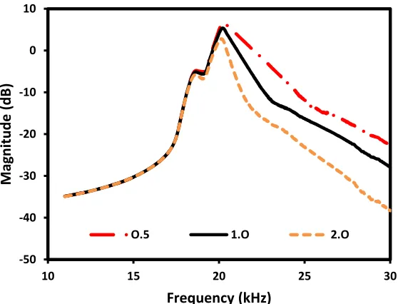
4.4 Effect of damping (Drive Mode) on resonance frequency
mx + dxxx + kxxx + kxy y + dxy y = ux + 2m Ωz y (11)
Here, damping along the drive axis is varied(Figure 13). When damping increases to
double, magnitude of resonance goes down by 10% and resonance frequency itself goes
down by 0.16%. It is obvious from the Figure 13 that the resonance frequencies do not
change that much but the steepness of the slope decreases as drive mode damping increases
after resonance frequencies. Here, “1” means reference damping (0.429e - 6 N s/m), “0.5”
means damping has been reduced by 50%, “2” means damping has been increased to
double. ‐0.1 ‐0.05 0 0.05 0.1
0 0.0001 0.0002 0.0003 0.0004 0.0005
Amplitude
Time (sec)
Figure 13: Effect of drive mode damping on resonance frequency
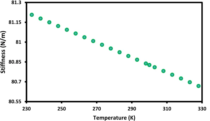
4.5 Effect of temperature variation on stiffness and damping
One key disadvantage of MEMS gyrosocpe is its high thermal sensitivity. The
frequency of oscillation drifts with temperture. Temperature variation mainly affects the
stiffness and damping of the supporting beams. Here investigation on the temperature
sensitivity for stiffness and damping is done. The variation of stiffness with temperature
can be modeled using simplified linear relationship of [4]
𝐾 𝑇 𝐾 1 𝑘∆𝑇 (12)
where K0 is the stiffness coefficient at reference temperature 300 K and k = 70 ppm.
Variation of damping coefficient with temperature can be modeled as [4] ‐50
‐40 ‐30 ‐20 ‐10 0 10
10 15 20 25 30
Magnitude
(dB)
Frequency (kHz)
d T d . 1.28 (13)
Where T is temperature in K , d is demping coefficient at reference temperature of 300 K.
Magnitude shows positive increasing trend with the increase of temperature when
stiffness and temperature relationship shows linear behaviour. The damping coefficient
within normal operating temperature range shows decreasing trend as temperature
increases (Figure 14).
4.6 Effect of temperature variation on stiffness coefficient
When the temperature increases, the atoms of the object gain significant amount of
Kinetic energy. Kinetic energy is a measure of the ability to move. This causes atoms to
move apart causing an increase in the area. When the area increases, the stress (Force /
Area) decreases. Young’s modulus E = Stress / Strain. As the numerator falls, the value of
E also falls. This is why Young's modulus decreases with increase in Temperature. As
spring stiffness is related to Young’s modulus, it decreases as the temperature increases.
Figure 14: Relationship between temperature and stiffness
When the stiffness changes by 0.70 %, magnitude changes by 0.378 %.
Figure 15: Relationship between stiffness and magnitude when temperature changes 80.55
80.7 80.85 81 81.15 81.3
230 250 270 290 310 330
Stiffness
(N/m)
Temperature (K)
9.3 9.6 9.9 10.2 10.5 10.8
80.75 80.85 80.95 81.05 81.15 81.25 81.35
Magnitude
(dB)
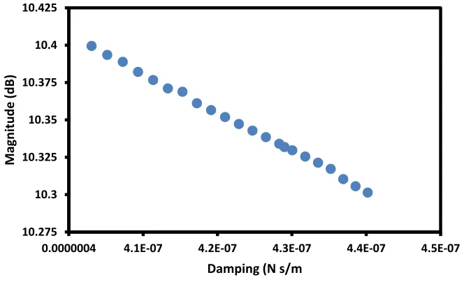
4.7 Effect of temperature variation on damping coefficient
When the temperature is raised from -40C to 60C, damping is going up by 9.22 %.
Figure 16: Relationship between temperature and damping
When the Damping changes by 9.22 %, magnitude changes by 0.92 %.
Figure 17: Relationship between damping and magnitude when temperature changes 3.98E‐07 4.05E‐07 4.13E‐07 4.20E‐07 4.28E‐07 4.35E‐07 4.43E‐07
230 250 270 290 310 330
Damping (N s/m) Temperature (K) 10.275 10.3 10.325 10.35 10.375 10.4 10.425
0.0000004 4.1E‐07 4.2E‐07 4.3E‐07 4.4E‐07 4.5E‐07
Magnitude
(dB)
4.8 Effect of mass variation on resonance frequency
Figure 18: Effect of mass variation on response curve
Here, m is varied from 75% (normalized value 0.75) to 125% (normalized value
1.25). The normalized value of tuned reference mass (0.57e -8 kg) is considered as 1. It is
observed that magnitudes at resonance frequencies show linear increasing trend (Figure
18) as mass decreases.
mx + dxx x + kxxx + kxy y + dxy y = ux + 2m Ωz y (11)
It is observed that if mass goes down by 50%, magnitude goes down by 5%. ‐50
‐35 ‐20 ‐5 10
10 20 30 40 50 60
Magnitude
(dB)
Frequency (kHz)
25% more than Ref. Mass
Ref. Mass
4.9 Effect of angular rate variation on sense frequency
Figure 19: Effect of angular rate variation on output signal
mx + dxx x + kxxx + kxy y + dxy y = ux + 2m Ωz y (11)
Angular rate has an impact on the performance of gyroscope output. As it is observed
in Figure 19 that with the variation of angular rate, amplitude of the sense output varies
significantly. It has been found that at 1 rad/s angular rate maximum amplitude is 0.0023,
at 3 rad/s angular rate maximum amplitude is 0.0070 and at 5 rad/s angular rate maximum
amplitude is 0.0117 which clearly showing an increasing trend. ‐0.00006
‐0.00003 0 0.00003 0.00006
0 0.0002 0.0004 0.0006 0.0008
Amplitude
Time
CHAPTER 5: CONTROLLER
Manufacturing defects and external disturbances degrade the performance of
MEMS gyroscope [27]. It is difficult to get actual value of resonance frequency due to
environmental effect which reduces the sensitivity of the gyroscope [28]. Neglecting these
issues will lead to achieve wrong angular velocity [29]. These disturbances reduce the
influence of the drive axis on the sense axis as well as the effect of Coriolis force. Hence,
practical control techniques are very attractive research area in the field of MEMS
gyroscopes [30].
Here, a sinusoidal signal is given in the drive direction to oscillate the proof mass
(Figure 20) and the sensed signal (Figure 21). We can see here that output signal is not
sinusoidal.
Figure 20: Input Signal (Drive Direction) ‐1
‐0.5 0 0.5 1
0.0003 0.000345 0.00039 0.000435 0.00048
Amplitude
Figure 21: Output Signal (Sense Direction)
Figure 22: Hypothetical Input Signal Figure 23: Hypothetical Expected Output Signal ‐0.025
‐0.015 ‐0.005 0.005 0.015
0.0003 0.000345 0.00039 0.000435 0.00048
Amplitude
Figure 24: Hypothetical Actual Output Signal Figure 25: Hypothetical Repaired Signal by
using Controller
For example, this is a hypothetical input signal in the drive direction as shown in
Figure 22. This is the expected hypothetical output signal in the sense direction as shown in Figure 23. But due to manufacturing defects and environmental noises, we got the hypothetical distorted output signal in the sense direction as shown in Figure 24. Controller can repair the actual distorted output signal and bring it back to expected output signal as shown in Figure 25.
.
Choice of Controller
Depending on the applications and complexity, different types of controllers are
PID controller
PID controllers are very suitable for linear systems but practically don’t produce
the best results when the system is nonlinear [30]. When PID controller is used with other
controller it can give highly accurate results [31].
Adaptive sliding mode controller
Nonlinearities are always present in dynamic systems. Typical PID controller
cannot handle these kind of nonlinearities. Adaptive controller can be used in these kind of
situations because of its ability to adjust the parameters according to changing system
dynamics. Robustness and insensitivity to external disturbances are notable features of
adaptive controller. However, its requirements for extensive complex model structure
discourages its use [32].
Neural controller:
Neural network consists of neurons. Their connections are weighted. Relationship
between neurons depends on their weighted sum of input and output [30]. Neural network
can learn and approximate nonlinear functions even in uncertain situations [33]. The
advantage of using neural control is that we need not to know the complex mathematical
model [34].
Neuro Fuzzy Controller
The neuro fuzzy systems inherit properties from both fuzzy systems and neural
networks without all disadvantages [27]. A neuro-fuzzy system simultaneously work
without precise mathematical model and can learn by itself [35]. When it is used for
nonlinear systems, its robustness can almost avoid the external disturbances [36].
Figure 26: Noise without controller at 1 rad/s angular rate
Figure 26 shows the presence of noise in the sense output of gyroscope. For
simplicity, a first order equation has been considered here. These noises make it difficult
to read the actual sense signals. To reduce or eliminate the noises controllers are used. Here
a continuous PID controller is used for noise reduction. Couples of trials have been made
to tune the PID controller. Table 2, Figure 27, Figure 28 and Figure 29 show relevant data
and figures. Peak time, peak value, rise time, slew rate, overshoot and undershoot
parameters have been compared to get the tuned value. 0.997
0.9985 1 1.0015 1.003 1.0045
1.5 2 2.5 3 3.5
Angular rate (rad/s)
Table 2: Signal characteristics for different P, I, D, N values
Trial Parameters
Peak Time (sec) Peak Value Rise Time (ms) Slew Rate(/s) Overshoot (%) Undershoot (%) 1
P 4
1.077 1.001 10.074 78.727 0.317 1.988 I 200
D 0.04
F 21000
2
P 8
1.07 1.001 4.610 171.950 -0.772 1.967 I 400
D 0.08
F 28000
3
P 12
1.068 1.001 2.983 265.630 -0.746 1.953 I 600
D 0.12
F 35000
4
P 16
1.067 1 2.204 359.441 -0.545 1.987 I 800
D 0.16
F 42000
5
P 20
D 0.20
F 49000
6
P 24
1.066 1 1.448 547.187 -2.252 1.971 I 1200
D 0.24
F 49000
7
P 2
1.907 1 14.909 53.123 0.083 1.993 I 102
D 0.02
(Trial 1)
(Trial 2)
0 0.2 0.4 0.6 0.8 1 1.2
1 1.02 1.04 1.06 1.08 1.1
Amplitude
(rad/s)
Time
0 0.2 0.4 0.6 0.8 1 1.2
1 1.02 1.04 1.06 1.08 1.1
Amplitude
(rad/s)
(Trial 3)
(Trial 4)
0 0.2 0.4 0.6 0.8 1 1.2
1 1.02 1.04 1.06 1.08 1.1
Amplitude
(rad/s)
Time
0 0.2 0.4 0.6 0.8 1 1.2
1 1.02 1.04 1.06 1.08 1.1
Amplitude
(rad/s)
(Trial 5)
(Trial 6)
0 0.2 0.4 0.6 0.8 1 1.2
1 1.02 1.04 1.06 1.08 1.1
Amplitude
(rad/s)
Time
0 0.2 0.4 0.6 0.8 1 1.2
1 1.02 1.04 1.06 1.08 1.1
Amplitude
(rad/s)
(Trial 7)
Figure 27: Step responses for different P, I, D, N values 0
0.2 0.4 0.6 0.8 1 1.2
1 1.02 1.04 1.06 1.08 1.1
Amplitude
(rad/s)
Figure 28: Signal characteristics for different P, I, D, N values ‐4
0 4 8 12 16
1 2 3 4 5 6 7
Units
Trial
Figure 29: Slew rate
Figure 30: Noise reduced after using after continuous PID controller at 1 rad/s angular
rate 0
100 200 300 400 500 600
1 2 3 4 5 6 7
Slew rate (/s)
Trial
0.997 0.998 0.999 1 1.001 1.002
1.5 2 2.5 3 3.5
Angular rate (rad/s)
The continuous PID controller has been tuned using the values shown below:
Table 3: Continuous PID controller tuned parameters
Source Values
Proportional (P) 3
Integrator (I) 102
Derivative (D) 0.02
Filter coefficient (N) 19747
Discrete PID controller also has been used for noise reduction (Figure 31).
Figure 31: Noise reduced after using after discrete PID controller at 1 rad/s angular rate
The continuous PID controller has been tuned using the values shown below (Table 4): ‐1E+157
‐5E+156 0 5E+156 1E+157
1.5 2 2.5 3 3.5
Angular rate (rad/s)
Table 4: Discrete PID controller tuned parameters
Source Values
Proportional (P) 3
Integrator (I) 102
Derivative (D) 0.02
Filter coefficient (N) 19747
Figure 32: Unit step response without controller 0
0.2 0.4 0.6 0.8 1 1.2 1.4 1.6 1.8
1 1.2 1.4 1.6 1.8 2
Amplitude
(rad/s)
Figure 33: Unit step response with PID controller
Table 5: Comparison between without controller and PID controller at transient zone
Without controller PID controller
Rise Time (ms) 28.269 14.909
Slew Rate (/s) 28.046 53.123
Overshoot (%) 4.737 0.083
Undershoot (%) -0.252 1.993
Peak Value 1.043 1
Peak Time (s) 1.056 1.907
0 0.2 0.4 0.6 0.8 1 1.2 1.4 1.6 1.8
1 1.2 1.4 1.6 1.8 2
Amplitude
(rad/s)
Figure 34: Comparison of signal characteristics between no controller and PID controller ‐20%
0% 20% 40% 60% 80% 100%
Rise Time (ms)
Slew Rate (/s)
Overshoot (%)
Undershoot (%)
Peak Value Peak Time (s)
Percentage
Signal Charecteristics
CHAPTER 6: CONCLUSION
This thesis investigates the effect of variation of suspending stiffness coefficients,
damping coefficients and temperature on the performance of MEMS gyroscopes.
Simulation results show how these parameters are affecting the error i.e. mismatch between
the input and sense signals which will help to design appropriate system parameters as well
as controllers to increase gyroscope accuracy. Simulation results also show that if stiffness
in the sense direction remains constant at 71.62 N/m, stiffness in the drive direction is
varied from 50% to 150%, the magnitudes at resonance frequencies show linear decreasing
trend and amplitudes decrease as stiffness increases. However, decreasing the stiffness
creates phase lag and distortion in output response. It is observed that if stiffness goes up
by 50%, resonance frequency goes up by 21% and magnitude goes down by 27%. It has
been observed that resonance frequency doesn’t change that much with the change of sense
mode stiffness. When damping increases to double, magnitude of resonance goes down by
10% and resonance frequency itself goes down by 0.16%. It is obvious from the
simulations that the resonance frequencies do not change that much but the steepness of
the slope decreases as drive mode damping increases after resonance frequencies. When
the temperature is raised from -40C to 60C, stiffness goes down by 0.70 % and when the
stiffness changes by 0.70 %, magnitude changes by 0.378 %. When the temperature is
raised from -40C to 60C, damping is going up by 9.22 % and when the damping changes
by 9.22 %, magnitude changes by 0.92 %.From the simulation result it is observed that
Temperature sensitivity can degrade resonance frequency and sense
magnitude.
Sense mode damping has little impact on the system.
Changing weight of the proof mass and drive mode damping can moderately
affect the magnitude of resonance frequency.
It can be said that according to the result, by adjusting only stiffness, the
system can be taken near optimum condition.
CHAPTER 7: FUTURE WORK
In the future, it is planned to extend this by comparing these simulation results with
the data obtained from physical experiments and implement an advanced controller like
fuzzy logic to minimize the noise, rise time, undershoot, overshoot and maximize the
gyroscope performance.
7.1 Why Fuzzy Logic Controller
Control system using fuzzy methodology can handle model uncertainties and
manufacturing imperfections. The fuzzy controller can work even without any precise
mathematical model [31]. The major limitations of Fuzzy Logic based controller are rules
must be available, cannot learn by itself [34].
7.2 How does fuzzy controller work?
Fuzzy logic generally used in uncertain nonlinear systems. It consists of several
Figure 35: A Fuzzy Logic System
Fuzzy logic algorithm:
1. Defining the linguistic variables
2. Developing membership functions
3. Developing rules
4. Transforming input data to fuzzy data using the membership functions
5. Getting the result from each rule
6. Combining all the results
7. Converting the combined result into non fuzzy data
Linguistic Variables
These are the variables whose values are natural words rather than numerical
numbers. A linguistic variable is segregated into several linguistic terms.
Membership Functions
Membership converts the non-fuzzy input data to fuzzy linguistic values and vice
versa. A fuzzy value can be the member of several sets at the same time. Different
membership functions are available like triangular, trapezoidal, piecewise linear, Gaussian,
singleton etc. [37].
Fuzzy Rules
Fuzzy rules control the output variable. A fuzzy rule consists of simple IF-THEN
Fuzzy Set Operations
The combination of fuzzy results are done by fuzzy set operations. If μA and μB are
the membership functions for fuzzy sets A and B, Table 6 contains possible fuzzy
operations for OR and AND. The operations for OR and AND operators are max and min.
For NOT operation Equation 14 is used for fuzzy sets.
𝜇 ̅ (x)=1-𝜇 (x) (14)
Table 6: Fuzzy Set Operations
OR (Union) AND (Intersection)
MAX Max(𝜇 𝑥 , μ x ) MIN Min x , μ x )
ASUM μ x μ x μ x μ x PROD μ x μ x
BSUM Min(1,μ x μ x ) BDIF Max(0,μ x μ x 1)
Combining individual results in to a final result is called inference. Different
methods are available for combining those results. Table 7 shows some methods for
combining the results.
Table 7: Accumulation Methods
Operations Formula
Maximum Max(μ x , μ x )
Bounded Sum Min(1, μ x μ x )
Defuzzification
This step converts the resulted fuzzy value to normal or crisp data. Like
Fuzzification, several Defuzzification methods are also available. The most popular ones
are shown in in Table 8 [38].
Table 8: Defuzzification Algorithms & variables
Variable Meaning Operation Formula
i Index
Center of
Gravity U= inf Smallest value
max Upper limit of defuzzification
min
Lower limit of
defuzzification
Center of
Gravity for
Singletons
∑ u μ
∑ μ
p Number of Singletons
sup Largest Value Left Most
Maximum
U= inf(u,), μ(u,)=sup(μ(u))
u Output Variable
U Result of Defuzzification
Right Most
Maximum U= sup(u
,), μ(u,)=sup(μ(u))
μ
Membership Function
REFERENCE
[1] "IRE Standards on Navigation Aids: Definitions of Inertial Navigation Terms,
1962," 62 IRE 12.S1 (IEEE 174), pp. 1-6, 1962.
[2] F. Braghin, F. Resta, E. Leo, and G. Spinola, "Nonlinear dynamics of vibrating
MEMS," Sensors and Actuators A: Physical, vol. 134, pp. 98-108, 2007/02/28/
2007.
[3] J. Fei and C. Batur, "A novel adaptive sliding mode control with application to
MEMS gyroscope," ISA Transactions, vol. 48, pp. 73-78, 2009/01/01/ 2009.
[4] M. Wen, W. Wang, Z. Luo, Y. Xu, X. Wu, F. Hou, et al., "Modeling and analysis
of temperature effect on MEMS gyroscope," in 2014 IEEE 64th Electronic
Components and Technology Conference (ECTC), 2014, pp. 2048-2052.
[5] J. Wang, S. Ban, and Y. Yang, "A Differential Self-Integration D-Dot Voltage
Sensor and Experimental Research," IEEE Sensors Journal, vol. 15, pp. 3846-3852,
2015.
[6] S. Woon-Tahk, S. Sangkyung, L. Jang Gyu, and K. Taesam, "Design and
performance test of a MEMS vibratory gyroscope with a novel AGC force
rebalance control," Journal of Micromechanics and Microengineering, vol. 17, p.
1939, 2007.
[7] W. Juan and J. Fei, "Adaptive fuzzy approach for non-linearity compensation in
MEMS gyroscope," Transactions of the Institute of Measurement and Control, vol.
[8] J. Collin, P. Davidson, M. Kirkko-Jaakkola, and H. Leppäkoski, "Inertial Sensors
and Their Applications," in Handbook of Signal Processing Systems, S. S.
Bhattacharyya, E. F. Deprettere, R. Leupers, and J. Takala, Eds., ed Cham: Springer
International Publishing, 2019, pp. 51-85.
[9] F. Khoshnoud and C. W. d. Silva, "Recent advances in MEMS sensor
technology-mechanical applications," IEEE Instrumentation & Measurement Magazine, vol.
15, pp. 14-24, 2012.
[10] "IEEE Standard Specification Format Guide and Test Procedure for Coriolis
Vibratory Gyros," IEEE Std 1431-2004, pp. 1-78, 2004.
[11] "IEEE Standard for Inertial Sensor Terminology," IEEE Std 528-2001, p. 0_1,
2001.
[12] C. Acar and A. Shkel, MEMS Vibratory Gyroscopes: Structural Approaches to
Improve Robustness (MEMS Reference Shelf): Springer Publishing Company,
Incorporated, 2008.
[13] M. Grewal and A. Andrews, "How Good Is Your Gyro [Ask the Experts]," IEEE
Control Systems Magazine, vol. 30, pp. 12-86, 2010.
[14] M. J. Ahamed, D. Senkal, A. A. Trusov, and A. M. Shkel, "Study of High Aspect
Ratio NLD Plasma Etching and Postprocessing of Fused Silica and Borosilicate
Glass," Journal of Microelectromechanical Systems, vol. 24, pp. 790-800, 2015.
[15] J. Liu, J. Jaekel, D. Ramdani, N. Khan, D. S. K. Ting, and M. J. Ahamed, "Effect
of Geometric and Material Properties on Thermoelastic Damping (TED) of 3D
[16] D. Senkal, M. J. Ahamed, M. H. A. Ardakani, S. Askari, and A. M. Shkel,
"Demonstration of 1 Million Q-Factor on Microglassblown Wineglass Resonators
With Out-of-Plane Electrostatic Transduction," Journal of Microelectromechanical
Systems, vol. 24, pp. 29-37, 2015.
[17] A. M. Shkel, D. Senkal, and M. Ahamed, "METHOD OF FABRICATING
MICRO-GLASSBLOWN GYROSCOPES," USA Patent US Patent
US9702728B2, 2017.
[18] J. Fei and C. Batur, A novel adaptive sliding mode control with application to
MEMS gyroscope vol. 48, 2008.
[19] W.-T. Sung, S. Sung, G.-I. Jee, and T. Kang, Design and performance test of a
MEMS vibratory gyroscope with a novel AGC force rebalance control vol. 17,
2007.
[20] J. Fei, M. Xin, and W. Juan, Adaptive fuzzy sliding mode control using adaptive
sliding gain for MEMS gyroscope vol. 35, 2013.
[21] Mathwork. (2018, 26 March). Simulink. Available: https:// www.mathworks.com
/products/simulink.html
[22] J. Fei, W. Dai, M. Hua, and Y. Xue, "System Dynamics and Adaptive Control of
MEMS Gyroscope Sensor," IFAC Proceedings Volumes, vol. 44, pp. 3551-3556,
2011/01/01/ 2011.
[23] M. R. Moghanni, J. Keighobadi, and A. Ghanbari, "Fuzzy Adaptive Sliding Mode
Controller for MEMS Vibratory Rate Gyroscope," IFAC Proceedings Volumes,
[24] R. Horowitz, New Adaptive Mode of Operation for MEMS Gyroscopes vol. 126,
2004.
[25] M. L. C. d. Laat, H. H. P. Garza, J. L. Herder, and M. K. Ghatkesar, "A review on
in situ stiffness adjustment methods in MEMS," Journal of Micromechanics and
Microengineering, vol. 26, p. 063001, 2016.
[26] J. Fei and H. Ding, "System Dynamics and Adaptive Control for MEMS Gyroscope
Sensor," International Journal of Advanced Robotic Systems, vol. 7, p. 29,
2010/12/01 2010.
[27] J. Fei and J. Zhou, "Robust Adaptive Control of MEMS Triaxial Gyroscope Using
Fuzzy Compensator," IEEE Transactions on Systems, Man, and Cybernetics, Part
B (Cybernetics), vol. 42, pp. 1599-1607, 2012.
[28] M. Fazlyab, M. Z. Pedram, H. Salarieh, and A. Alasty, "Parameter estimation and
interval type-2 fuzzy sliding mode control of a z-axis MEMS gyroscope," ISA
Transactions, vol. 52, pp. 900-911, 2013/11/01/ 2013.
[29] R. Zhang, T. Shao, W. Zhao, A. Li, and B. Xu, Sliding Mode Control of MEMS
Gyroscopes Using Composite Learning vol. 275, 2017.
[30] T. T. Xie, H. Yu, and B. M. Wilamowski, "Comparison of Fuzzy and Neural
Systems for Implementation of Nonlinear Control Surfaces," in Human – Computer
Systems Interaction: Backgrounds and Applications 2: Part 2, Z. S. Hippe, J. L.
Kulikowski, and T. Mroczek, Eds., ed Berlin, Heidelberg: Springer Berlin
[31] F. Gouadria, L. Sbita, and N. Sigrimis, "Comparison between self-tuning fuzzy PID
and classic PID controllers for greenhouse system," in 2017 International
Conference on Green Energy Conversion Systems (GECS), 2017, pp. 1-6.
[32] J. Fei and H. Ding, "Adaptive sliding mode control of dynamic system using RBF
neural network," Nonlinear Dynamics, vol. 70, pp. 1563-1573, 2012/10/01 2012.
[33] R. Zhang, T. Shao, W. Zhao, A. Li, and B. Xu, "Sliding mode control of MEMS
gyroscopes using composite learning," Neurocomputing, vol. 275, pp. 2555-2564,
2018/01/31/ 2018.
[34] M. Nagai, A. Moran, Y. Tamura, and S. Koizumi, "Identification and control of
nonlinear active pneumatic suspension for railway vehicles, using neural
networks," Control Engineering Practice, vol. 5, pp. 1137-1144, 1997/08/01/ 1997.
[35] T. R. Kiran and S. P. S. Rajput, "An effectiveness model for an indirect evaporative
cooling (IEC) system: Comparison of artificial neural networks (ANN), adaptive
neuro-fuzzy inference system (ANFIS) and fuzzy inference system (FIS)
approach," Applied Soft Computing, vol. 11, pp. 3525-3533, 2011/06/01/ 2011.
[36] W. Yan, S. Hou, Y. Fang, and J. Fei, "Robust adaptive nonsingular terminal sliding
mode control of MEMS gyroscope using fuzzy-neural-network compensator,"
International Journal of Machine Learning and Cybernetics, vol. 8, pp. 1287-1299,
2017/08/01 2017.
[37] C. Byoung-doo, P. Sangjun, K. Hyoungho, P. Seung-Joon, P. Yonghwa, L.
Geunwon, et al., "The first sub-deg/hr bias stability, silicon-microfabricated
and Microsystems, 2005. Digest of Technical Papers. TRANSDUCERS '05., 2005,
pp. 180-183 Vol. 1.
[38] J. M. Mendel, "Fuzzy logic systems for engineering: a tutorial," Proceedings of the
IEEE, vol. 83, pp. 345-377, 1995.
VITA AUCTORIS
NAME: Md. Imrul Kaes
PLACE OF BIRTH: Dhaka, Bangladesh
YEAR OF BIRTH: 1985
EDUCATION: Bachelor in science in industrial & production
engineering, Bangladesh University of
Engineering & Technology, Dhaka,
Bangladesh.
Master of engineering in industrial engineering,