Modeling and Control Strategy of the
Modular Multilevel Converter
P.Praveen Kumar1, B.Vamsikrishna2, A.Bindu Madhavi 3, K.Ram Mohan 4
Assistant Professor, Department of EEE, GMR Institute of Technology, Rajam, Andhra Pradesh, India1 UG Student, Department of EEE, GMR Institute of Technology, Rajam, Andhra Pradesh, India2,3,4
ABSTRACT:The aim of this project is the analysis of a Modular Multilevel Converter (MMC) and the development of a control scheme for energy stored. The analysis is based on the use of a simplified circuit constituted by a single leg of the converter where all the modules in each arm are represented by a single variable voltage source. Control scheme are is focusing on the balancing between upper and lower arm voltage and on the control of the overall energy stored in converter leg.
KEYWORDS: Sub modulus, Chopper cells, Switching Frequency.
I.INTRODUCTION
Power conversion the recent attention of the environment protection and preservation increased the interest in the energy power generation from renewable sources wind power systems and solar power systems are defusing and are supposed to occupy an increasingly important role.
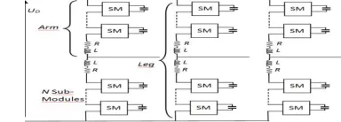
The multilevel approach guarantees a reduction of output harmonics due to sinusoidal output voltage. Many multi-level converter topologies have been investigated in these last years [1], having advantages and disadvantages during operation or when assembling the converters. To solve the problems of conventional multi-level converter a new MMC topology was proposed in [2]-[5], describing the operation principle and performance under different operating conditions. A simple schematic of this converter with N modules per arm is shown in Fig. 1. The MMC proposed in [2]-[5] is one of the most promising power converter topology for high power applications in the near future, particularly in HVDC links (e.g. transmission of offshore wind power, among others). Siemens has a plan of putting this converter into practical applications with the trade name “plus”. The system configuration of the HVDC-plus has a power of 400 MVA, a dc link voltage of 200 kV, and each arm composed of 200 cascaded chopper cells [6]. This converter topology has been investigated by several research teams lately [7]-[12]. The aim of this paper is to accomplish the stable voltage control of the MMC in all operating conditions and the theoretical analysis is based on the circuit model proposed in [8], The approach is based on using a continuous model, where all modules in each arm are represented by variable voltage sources, and PWM effects are neglected.
II.DESCRIPTION AND PRINCIPLE OF OPERATION OF MMC
The typical structure of the MMC is shown in the fig.1 and the configuration of a sub modulus(SM)is given in fig2.Each SM is a simple chopper cell composed of two IGBT switches(T1 and T2),two anti-parallel diodes
Fig 1: Schematic of a three-phase Modular Multi-level Converter
The output voltage is given by U0
Uo=Uc if T1is on and T2 is off
The configuration with T1and T2 both ON should not be considered because it determines a short circuit across the capacitor. Also the configuration with T1 and T2 is not useful as it produces the output voltage depending on the current direction .In the MMC the number of the output voltage is related to the number of series connected SMS. .
Fig 2: chopper cell of a sub-module
III.MATHEMATICAL MODEL OF THE MMC
The typical structure of the MMC can be summarized in to three levels: 1. sub-modules SM (the lower level,usually Chopper cells) 2. arm (second level of the converter, half of the leg-phase) 3. leg (can be considered one phase)
If a two level control structure is considered ,for instance a Master Slave structure ,lower level of control is used to sub module level ,instead upper level of control deals with arm leg voltage and current control level
II , III. providing that the lower level control for the sub modules is present ensuring that all capacitors are equally charged.
The most of the stimulations are based on the switched and discrete models .they have two advantages
1) Discrete models do not allow an analytical approach to model the converter and to design the control system. 2) Numerical solutions of complex converter configuration using a high number of the SMS require considerable
simulation time.
A continuous model can overcome these disadvantages. to understand the operation of the converter it is necessary to write the voltage current equations. To determine a continuous model suitable to design a control scheme. In the following, an analysis is carried out with the aim to control the upper and lower arm voltages, using the continuous model presented in [8].
Ideal capacitance of the arm should be:
N C
C arm .
(1)
The effective capacitance of the arm is dependent on the insertion index .so it can be written as:
) (t n C C
arm m
(2)
where the m apex means the number of the arm. It would be possible to have a full representation of the MMC converter, including operation of each sub-module.
A simpler way would be to consider a continuous model, but 2 important assumptions are necessary in order to develop this approach:
1. The switching frequency is much higher than the frequency of the output voltage
2. The resolution of the output voltage is small, compared to the amplitude of the output voltage.
Assuming 1 and 2, it’s possible to create a continuous model .
ucm = n(t) uc∑(t)
(3)
m c t i dtt) ( ) ( du C with ) (t n C C arm m
(4)
current in the upper arm is denoted by iu
current in the lower arm is denoted by iL
now applying kcl we get:
V CU U U V
D n u u
dt di L Ri u 2
(5)
V CL L U LD n u u
dt di L Ri u 2
(6)
now diff the above equation
L CLCU U diff D diff
u
L
n
u
L
n
i
L
R
L
u
dt
di
2
2
2
(7)
V arm L diff arm L CL
i
C
n
i
C
n
dt
du
(8)
(9)
In order to solve the system of equations (9) the load current should be known. Here, the following alternating current is assumed as the output load current.iV(t) = iV
̂(t)cos(ω
Nt+ⱷ)As a consequence, assuming the capacitor voltages of all modules equal to the reference value, the sum of the voltages of upper and lower arms is always equal to the DC voltage uD.
When assuming a constant DC voltage, actually it is possible to generate output voltages having a number of levels equal to 2N+1, whereas the number of levels must be reduced to N+1 if the the DC voltage has to be kept under control by the converter itself.
A CONTROL STRATEGY:
By adding and subtracting equations (7) to (8), it is possible to obtain two equations that clearly explain a possible approach to MMC control:
V
u
=dt di L i R u u V V CL CU 2 2
2
(10)
2 2 CU CL D diff
diff u u u
Ri dt di
L (11)
It is opportune for control purposes to obtain an expression of upper and lower arm voltages in which this voltage difference is included. Starting from (8) and substituting the upper current with
diff V
U i
i
i
2
Leads to
2 2
2 2 2 2 CU arm CU CU CU u C u N C N u c N W (12)
2 2
2 2 2 2 CL arm CL CL CL u C u N C N u c N W (13) Considering now power equations of both upper and lower arms, it is possible to write:
CU CLC
W
W
W
(16)
CU CLC
W
W
W
(17)B: CONSIDERATION ABOUT CONTROL STRATEGY AND MODEL
The equations wrote and discussed in previous section lead to a continuous model, suitable for analysis and understanding of operation principle of the MMC.
From equations (14) and (15) it becomes clear that the input variables, or rather modulation indexes, influence dynamics of the energy as a non-linear input.
6
Fig4:Input Control Relationship
Neglecting this low pass filter it is possible to consider that input variables are a “square” input The control strategy implemented is a linear control.
Two different loops will be implemented, the first one to control the overall energy of the MMC leg, the second to control the balance between upper and lower arms of the phase-leg.
The interaction between two loops may lead to instability: because of the non-linear configuration of system equations.
IV.DEVELOPMENTOFAMATLABMODEL
Starting from equations and discussions of Chapter III, it is possible to define a simple dynamic model of one phase of the converter.
(9)
diff V D diff V CU U
CU i u i i u e u
dt dW
2 2
(14)
V g g
g g
g V V
i L R
L u
L u dt di
(15)
Equation (15) is the output voltage equation, where is the grid voltage, and Rg, Lg the parameters of the line connecting MMC to the grid.
The previous equations are implemented on Stimulant.
A.FIRST MODEL: CONVERTER OPERATION AND MODEL VERIFICATIONS
The first system implemented in MATLAB-Stimulant includes only the equations in (9).
It will be shown that control strategy implemented is almost independent from parameters changes; however it is easier to start solving the problem from a small scale system.
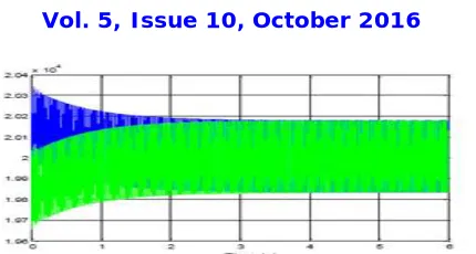
No control loop is implemented yet, and the converter is not able to keep the capacitor voltage to the initial value. Arm voltages waveforms are shown in Fig5
Fig 5: Upper (Blue) and Lower (Green) Arm Capacitance Voltage
B. SECOND MODEL: ENERGY CONTROL
The second system implemented includes energy equations (11) propose an energy control strategy, to obtain a stable single-phase leg of the converter. As deducted by equations (10) and (11), differential current can be controlled by a differential; this voltage will not affect the AC (output) side .Thus, a simple but efficient control strategy controls overall energy stored and the balance between upper and lower arm energy through the differential current, using the differential voltage as intermediate control input.From equations (16) and (17), rewritten in the following for convenience, it is possible to understand how to control properly the overall energy and the energy balance.
D diff
diff V V Ci e i u u dt dW
2
(16) diff
V V diff D
C u u i e i
dt dW
2
2
(17) In equation (16), differential current multiplies the DC voltage.In equation (17), differential current multiplies the output so an AC component of differential current is used in order to control the balance between upper and lower energy .
An important consideration must be performed: both loops implemented to control energy behavior include saturation.
C THIRD MODEL : OUTPUT POWER CONTROL
A MATLAB Embedded block is added in order to implement the output current dynamic equation; then, a resonant controller is applied to output current error,. The controller is composed of two main contributions: a proportional, and a resonant part. The Bode diagram is shown below in
Fig6: Bode Diagram of Resonant Controller
D. SIMULATION RESULTS
The Fig.7, shows the behavior of differential current.
Fig7: Differential Current Waveform (A) E. FOURTH MODEL- MEGA- WATT SYSTEM
The MW power system requires only changing the limitations on the differential voltage available: as much as the power increases, as much the differential voltage, used to control the energy stored in the system, has to increase. The control system scheme remains exactly the same, and will be proven to be reliable and tightly dependent with system parameters: however, an important consideration has to be deepened about system project.
F. CAPACITANCE VOLTAGE RIPPLE RELATIONSHIP
Starting from voltage derivate equations in (9), here rewritten for convenience,
V arm
L diff arm
L CL
i C
n i
C n dt du
(8)
it is possible to find a relationship between voltage and arm capacitance. Considering only the upper arm voltage
o diff
I
i
(18)
)
sin(
t
I
i
V
M
(19)
For the differential current, it is possible to consider only the DC component: this component is used to maintain the capacitor voltage to a constant value.
o
M o u arm o CU
CU n I I t d t
C u
u 1 sin() ()
(20) Where modulation index can be considered as
2 ) ( 1 )
(t m t nU
(21) With the hypothesis that
)
sin(
)
(
t
wt
m
(22) Sub(40)and (41) in(39)we get:
arm M o
o CU CU
C I I
u u
2
1 8 1
2
(23)
With this equation it is possible to understand the system operation and thus to size properly the capacitance of the arm, once assigned output current and calculated the DC component of differential current, in order to satisfy voltage ripple constraints.
G. SIMULATION RESULTS:
The only change can be seen in the order of magnitude of variables observed. Figs.8
Fig8: overall energy(joules)steady state waveform
fig 9: upper (blue)and lower (green) arm voltage (V) in steady state condition
H.SIMULATION RESULTS: LVRT
Last simulations shown in this are related to Low Voltage Ride Through issue: in order to simulate this operating condition, grid voltage is set to zero for 200 ms as represented in Fig.10.
Fig10: Grid Voltage (V) during LVRT
Actually, the system behavior fulfills expectations: as shown in Fig. 11, the overall energy is stable and has a small transient, leading to a steady-state condition.
Fig11:Overall Energy (Joule): Behavior in LVRT condition
V. MODELING PRINCIPLES AND EQUATIONS
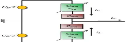
A new simplified schematic of the MMC leg is proposed and shown in below figure.
By following Kirchhoff’s: laws
p p p P o
P R i
dt di L V
V (24)
N N N N o
N
R
i
dt
di
L
V
V
(25)N P
o
i
i
Defining Sp and Sn as modulation indexes, respectively of upper and lower arms, it is possible to write:
P P P
DC
V
S
E
E
(27)N N
N
S
E
V
(28)VI. CONCLUSIONS
The analysis of a Modular Multilevel Converter (MMC) for wind farm applications and the development of a control scheme to monitor the energy behavior is done and is based on the use of a simplified circuit, constituted by a single leg of the converter, where all the modules in each arm were represented by a single variable voltage source. The circuit model was derived as a system of differential equations, used for analyzing both the steady state and dynamic behavior of the MMC, from voltages and thus energy point of view.
Preliminary analysis was carried out following the modeling approach proposed in [8]. Using this model, the system behavior has been studied and a possible energy control scheme has been developed.
REFERENCES
[1] J. Rodriguez, J. S. Lai, and F. Z. Peng, “ Multilevel Inverters: a survey of topologies, controls, and applications. “ IEEE Trans. Ind. Electronics, vol. 49, no. 4, pp. 724-738, August 2002.
[2] A. Lesnicar, and R. Marquardt, “An Innovative Modular Multilevel Converter Topology Suitable for a Wide Power Range”, IEEE PowerTech Conference, Bologna, Italy, June 23-26, 2003.
[3] A. Lesnicar, and R. Marquardt, “A new modular voltage source inverter topology”, EPE 2003, Toulouse, France, September 2-4, 2003. [4] R. Marquardt, and A. Lesnicar, “New Concept for High Voltage - Modular Multilevel Converter”, IEEE PESC 2004, Aachen, Germany, June 2004.
[5] M. Glinka and R. Marquardt, “A New AC/AC Multilevel Converter Family”, IEEE Transactions on Industrial Electronics, vol. 52, no. 3, June 2005.
[6] B. Gemmel, J. Dorn, D. Retzmann, and D. Soerangr, “Prospects of multilevel VSC technologies for power transmission”, in Conf. Rec. IEEE-TDCE 2008, pp. 1-6.
[7] M. Hagiwara, H. Akagi “PWM Control and Experiment of Modular Multilevel Converters”, IEEE PESC 2008, Rhodes, Greece, June 2008. [8] A. Antonopoulos, L. Angquist, and H.-P. Nee, “On dynamics and voltage control of the modular multilevel converter,” European Power Electronics Conference (EPE), Barcelona, Spain, September 8-10, 2009.
[9] G.Bergna, M.Boyra, J.H.Vivas, “Evaluation and Proposal of MMC-HVDC Control Strategies under Transient and Steady State Conditions” [10] P.Munch, S.Liu, M.Dommaschk “Modeling and Current Control of Modular Multilevel Converters Considering Actuator and Sensor Delays” [11] M.Hagiwara, R.Maeda, H.Akagi, “Control and Analysis of the Modular Multilevel Cascade Converter Based on Double-Star Chopper-Cells (MMCC-DSCC)”