Efficiency of Bat Optimization Algorithm in
Optimal Reactive Power Dispatch Problems
Dr. S. Sakthivel,Me.,Ph.D., Dr. S.Saravanan,Me.,Ph.D., P. Dhivyabharathi,
Professor and Head/ EEE(PG), Dept. of Electrical and Electronics Engineering, Muthayammal Engineering College,
Namakkal, Tamil Nadu, India
Professor and Head/ EEE(UG), Dept. of Electrical and Electronics Engineering, Muthayammal Engineering College,
Namakkal, Tamil Nadu, India
PG Scholar, Dept. of Electrical and Electronics Engineering, Muthayammal Engineering College, Namakkal,
Tamil Nadu, India
ABSTRACT: In this paper, the recent metaheuristic algorithm of bat optimization algorithm(BOA), is implemented for solving optimal reactive power dispatch (ORPD) problems. BOA can outperform several robust and efficient metaheuristic algorithms in solving engineering problems. ORPD problem is taken as a multi-modal and constrained optimisation problem with large number of control variables. Real power loss minimization and sum of voltage deviation minimization are the objectives of ORPD problem. The proposed algorithm was tested on the standard IEEE 30 and 57 bus power systems. The simulation results prove the outperformance of BOA over other algorithms compared from the literatures.
KEYWORDS: Optimal reactive power dispatch, Bat optimization algorithm loss minimization, voltage deviation minimization.
I. Introduction
Solution of optimal power flow (OPF) problem is very important in operation and planning of power systems that was introduced in 1960s [1-6]. ORPD problem is a sub set of optimal power flow problems [7, 8]. This problem is taken by large number of researcher across the world [9-12]. Because of the economic importuned of the ORPD problem only this of must important [9]. The aim of ORPD is to find the optimal values for generator bus voltages, transformers tap positions and VAR outputs from compensating devices for achieving low loss levels [9-11, 13-16].The problem is highly nonlinear and equality and inequality constraints are handled. These constraintsare represented as the power flow equations[17]. The problem has discontinued variables of transformer tap position and VAR compensator and continues variables of generator bus voltages [17, 18].
The rest of the paper is organized as follows: Section 2 describes the ORPD mathematical problem; Section 3 explains the proposed BOA for solving ORPD problem; Section 4 is devoted to the numerical results and discussions, finally, conclusions are drawn in the last section.
II. ORPD MATHEMATICAL PROBLEM
The objective of this work is to improve the stability of the system by minimizing the active power loss and the sum of load bus voltage deviation. The two objectives are considered separately.
2.1 Objective function
The objective function of this work is to find the optimal control variables values that minimizes the active power loss and voltage deviation at load buses.
2.1.1Active power loss minimization (PL)
The total active power of the system can be calculated as follows [19].
Where, NLis the total number of lines in the system; Gk is the conductance of the line ‘k’; Viand Vj are the magnitudes of the sending end and receiving end voltages of the line; δiand δj are angles of the end voltages.
2.1.2 Load bus voltage deviation minimization (VD)
Load bus voltage magnitude should be maintained within the allowable range to ensure quality of service [20]. Voltage profile can be improved by minimizing the deviation from the reference value (it is taken as 1.0 p.u. in this work).
2.2 Constraints
This ORPD optimization problem is subjected to the following equality and inequality constraints. 2.2.1. Equality constraints:
Power Flow Constraints:
2.2.2 Inequality constraints: Voltage Constraint:
Transformer tap constraint:
Shunt VAR constraint:
2 2
1
[
2
cos(
)]
(1)
L
N
L k i j i j i j
k
P
G V
V
VV
1
|(
) |
(2)
PQ
N
i ref K
VD
V
V
1
cos(
)
(3)
B
N
Gi Di i ij ij ij j i
j
P
P
VV Y
1
sin(
)
(4)
B
N
Gi Di i ij ij ij j i
j
Q
Q
VV Y
min max
;
(5)
i i i B
V
V V
i N
min max
;
(6)
i i i T
Transmission line flow limit:
In this research, power loss and total voltage deviation indexes have been used as objective function for ORDP problem. Control variables of the ORPD problem include VG, voltage at PV buses; T, transformer tap settings; QC, vector of shunt capacitor/inductor.
In this problem, equality constraints are active power balance equation and reactive power balance equation that are considered during power flow calculations. The inequality constraints considered in this problem are as follows.
III. BAT OPTIMIZATION ALGORITHM
3.1 Bat Algorithm
The bat algorithm is a swarm intelligence based method introduced in ref.[21]. This optimization algorithm is developed by theecholocation behavior of bats in searchingtheir prey. Bats emit a very loud sound pulse and listen to the echo returning from the prey/object. Bats fly randomly using frequency, velocity and position to search for prey. Pulse rate and loudness differ depending on the type of the bat. The bat algorithm is formulated imitating the ability of bats to find their prey.Each bat in bat algorithm represents a potential solution in the population of solutions.
Frequency, velocity and position ofeach bat in the population are updated for the next generation. It means that the bat algorithm uses a frequency tuningtechnique to provide the diversity of the solutions in the population. The bat algorithm has the advantage of combining apopulation-based algorithm with local search.
The role of pulse rate and loudness in this algorithm is to control the equalcombination of population-based and local search processes. This algorithm employs the variations of pulse rates and loudness of bats to try to balance the exploration and exploitation during the search process. The simplifications and idealization rules of bat behavior that are considered and proposed are taken from [22].
The algorithm involvesa progression of generations, where a set of solutions undergo modifications through random change of the signal bandwidth which is increasedusing harmonics. The loudness and pulse rate are updated when the new solution is accepted. The frequency, velocity andposition of the solutions are computed based on following formulas:
The value of β is a randomly chosen between [0, 1],firepresents the frequency of theith bat that controls the speed and
rangeof movement of the bats,ViandXiare the velocity and position ofith bat, respectively, andX*corresponds to the globalbest at time stept.
Local search is used in order to maintain the diversity of the solutions in the population.
The local search is applied to the solutions under consideration of a certain condition in the bat algorithm. This local searchfollows the random walk as given in Eq. (4).
min max
;
(7)
i i i
C C C C
Q
Q
Q
i
N
max 1
;
(8)
i i
S
S
i
N
min
(
max min) ,
(9)
i
f
f
f
f
1
*
(
) ,
(10)
t t t
i i i i
V
V
X
X
f
1
(11)
t t t
i i i
Where is a random number lies between [-1,1] that controls the direction and power of the random walk andAt denotes the average loudness till now.
The pulse rateriand the loudnessAiare updated in each iteration. The loudness decreases when a bat finds itsprey while the pulse rate increases at the same time. The loudnessAiand pulse rateriare updated according to the followingequations. Here, ‘a’and‘c’are constant values and are taken from a range ofaα [0,1]andγ>0. In our work, both values of‘a’and‘c’are set to 0.9 as in[43].
3.2 BOA algorithm implementation for ORPD problem
Bat algorithm is proposed to find minimum loss and voltage deviationby adjusting the decision variables:
Step 1: Initialize the number of population including bat position Xiand velocity Vi. Here,Xiis defined as the set of Vi, Tiand Qci. set theinitial value of velocity vi= (0).
Step 2: Set the initial frequencies fi, pulse rates ri and the loudness Ai for each bats.
Frequency shouldrespect its lower and upper bounds condition fmin ≤ fi ≤ fmax. In this problem fmin and fmax defined as 2 and 10 respectively.
Pulse ri is taken in range [0,1], while loudness varies in range [Amin, A0]. Amin is minimum value and A0 large
positive; in this case [Amin, A0] = [0, 20].
Step 3: Compute fitness value for each bat population which is the total power loss or total voltage deviation using Eqns. 1 and 2.
Step 4: Sort the population according to the ascending order of the total loss or voltage deviation and find the global best X∗.
Step 5: Modify frequency of bat population using Eqn. (9).Update Velocity using (10) and location using (11).
Step 6: if(rand >ri)
Step 7: Generate local solution around the global best solution using Eqn. (12)
Step 8: End if
Step 9:Calculate fitness value from new solution using Eqns. (1) and (2).
Step 10:if (rand <Ai &f(Xi) <f(X∗))
Step 11:Accept the new solution
Step 12:Increase ri and Ai by using (13)
(12)
t
new old
X
X
A
1 1 0
,
[1 exp(
)],
(13)
t t t
i i i i
A
A
r
r
t
Step 13: End if
Step 14:Print the results.
IV. NUMERICAL RESULTS AND DISCUSSIONS
To demonstrate the performance and effectiveness of the proposed BOA based approach, it has been applied for ORPD problems in IEEE 30 and 57 bus power systems. The parameters of these case studies are taken from [23]. The BOA algorithm has been implemented in MATLAB R2009b computing environment and the simulations are run using a core i5 based 4GB RAM computer. The population size is set to 50 and the maximum number of iterations taken as 300.
4.1. IEEE 30 bus power system
The single line diagram of the system is given in Fig. 1. In this section, the results obtained from IEEE 30 bus power system are presented. Generator data, line data, load data, reactive power sources, voltage magnitudes of buses and transformer tap settings can be found in ref. [23]. IEEE 30-bus power system has 19 control variables. There are 6 generator bus voltages, 4 transformer tap settings and 9 SVC devices in the test system. The total real power demand of the system in base load condition is 2.834 p.u.
4.1.1.Active power loss minimization
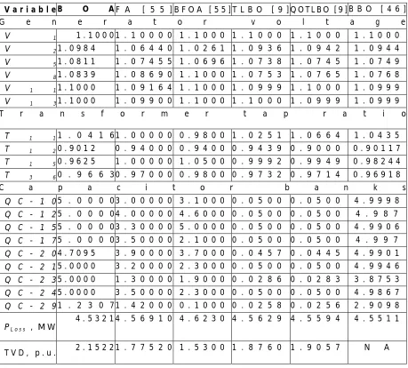
This section discusses the performance of BOA algorithm in active power loss minimization as the objective function. The results reported by the algorithm are given in Table 1. The best results achieved by BOA method has been compared with that of other algorithms in Table 1. The bestactive power loss achieved by the BOA is 4.5321 MW which is less than that what is produced by other algorithms mentioned in the Table 1.
Table 1
Optimal parameter settings for loss minimization in IEEE 30 bus system
V a r i a b l e B O A F A [ 5 5 ] B F O A [ 5 5 ] T L B O [ 9 ] Q O T L B O [ 9 ] B B O [ 4 6 ]
G e n e r a t o r v o l t a g e
V 1 1 . 1 0 0 0 1 . 1 0 0 0 0 1 . 1 0 0 0 1 . 1 0 0 0 1 . 1 0 0 0 1 . 1 0 0 0
V 2 1 . 0 9 8 4 1 . 0 6 4 4 0 1 . 0 2 6 1 1 . 0 9 3 6 1 . 0 9 4 2 1 . 0 9 4 4
V 5 1 . 0 8 1 1 1 . 0 7 4 5 5 1 . 0 6 9 6 1 . 0 7 3 8 1 . 0 7 4 5 1 . 0 7 4 9
V 8 1 . 0 8 3 9 1 . 0 8 6 9 0 1 . 1 0 0 0 1 . 0 7 5 3 1 . 0 7 6 5 1 . 0 7 6 8
V 1 1 1 . 1 0 0 0 1 . 0 9 1 6 4 1 . 1 0 0 0 1 . 0 9 9 9 1 . 1 0 0 0 1 . 0 9 9 9
V 1 3 1 . 1 0 0 0 1 . 0 9 9 0 0 1 . 1 0 0 0 1 . 1 0 0 0 1 . 0 9 9 9 1 . 0 9 9 9
T r a n s f o r m e r t a p r a t i o
T 1 1 1 . 0 4 1 6 1 . 0 0 0 0 0 0 . 9 8 0 0 1 . 0 2 5 1 1 . 0 6 6 4 1 . 0 4 3 5
T 1 2 0 . 9 0 1 2 0 . 9 4 0 0 0 0 . 9 4 0 0 0 . 9 4 3 9 0 . 9 0 0 0 0 . 9 0 1 1 7
T 1 5 0 . 9 6 2 5 1 . 0 0 0 0 0 1 . 0 5 0 0 0 . 9 9 9 2 0 . 9 9 4 9 0 . 9 8 2 4 4
T 3 6 0 . 9 6 6 3 0 . 9 7 0 0 0 0 . 9 8 0 0 0 . 9 7 3 2 0 . 9 7 1 4 0 . 9 6 9 1 8
C a p a c i t o r b a n k s
Q C - 1 0 5 . 0 0 0 0 3 . 0 0 0 0 0 3 . 1 0 0 0 0 . 0 5 0 0 0 . 0 5 0 0 4 . 9 9 9 8 Q C - 1 2 5 . 0 0 0 0 4 . 0 0 0 0 0 4 . 6 0 0 0 0 . 0 5 0 0 0 . 0 5 0 0 4 . 9 8 7 Q C - 1 5 5 . 0 0 0 0 3 . 3 0 0 0 0 5 . 0 0 0 0 0 . 0 5 0 0 0 . 0 5 0 0 4 . 9 9 0 6 Q C - 1 7 5 . 0 0 0 0 3 . 5 0 0 0 0 2 . 1 0 0 0 0 . 0 5 0 0 0 . 0 5 0 0 4 . 9 9 7 Q C - 2 0 4 . 7 0 9 5 3 . 9 0 0 0 0 3 . 7 0 0 0 0 . 0 4 5 7 0 . 0 4 4 5 4 . 9 9 0 1 Q C - 2 1 5 . 0 0 0 0 3 . 2 0 0 0 0 2 . 3 0 0 0 0 . 0 5 0 0 0 . 0 5 0 0 4 . 9 9 4 6 Q C - 2 3 5 . 0 0 0 0 1 . 3 0 0 0 0 1 . 9 0 0 0 0 . 0 2 8 6 0 . 0 2 8 3 3 . 8 7 5 3 Q C - 2 4 5 . 0 0 0 0 3 . 5 0 0 0 0 2 . 3 0 0 0 0 . 0 5 0 0 0 . 0 5 0 0 4 . 9 8 6 7 Q C - 2 9 1 . 2 3 0 7 1 . 4 2 0 0 0 0 . 1 0 0 0 0 . 0 2 5 8 0 . 0 2 5 6 2 . 9 0 9 8
PL o s s , M W
4 . 5 3 2 1 4 . 5 6 9 1 0 4 . 6 2 3 0 4 . 5 6 2 9 4 . 5 5 9 4 4 . 5 5 1 1
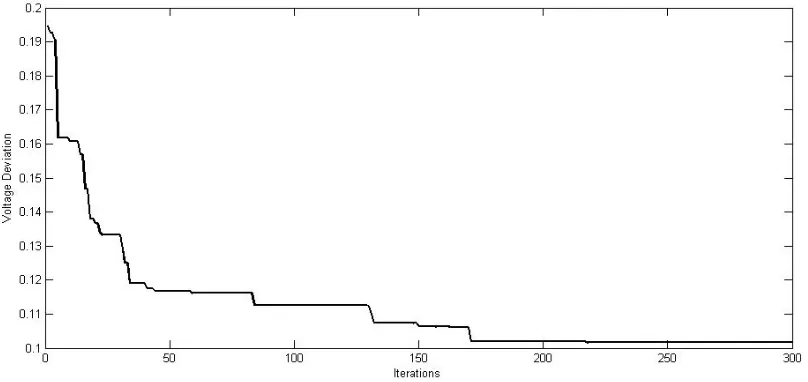
The algorithm takes about 150 iterations to get converged to the global best results indicating the reliable
convergence quality.This characteristic is depicted in Fig. 2.
Fig. 2 –Convergence quality of BOA in loss minimization in IEEE 30 bus system
4.1.2.VD Minimization
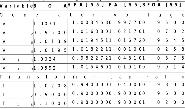
Sum of voltage deviation at all the load buses of the system is the objective taken in this case. The strength of the proposed algorithm is proved by comparing its results with other algorithms like HFA, FA, BFOA.Performance of the BOA algorithm is better than FA and BFOA algorithms. However, voltage deviation minimization by the proposed method is not better than the HFA algorithm.
Table 2
Optimal parameter settings for voltage deviation in IEEE 30 bus system
V a r i a b l e B O A H F A [ 5 5 ] F A [ 5 5 ] B F O A [ 5 5 ]
G e n e r a t o r v o l t a g e
V 1 1 . 0 0 3 1 1 . 0 0 3 4 5 8 0 . 9 9 7 7 0 0 . 9 5 0 0
V 2 0 . 9 5 0 0 1 . 0 1 6 3 8 0 1 . 0 2 1 7 0 1 . 0 7 0 2
V 5 1 . 0 1 3 9 1 . 0 1 9 4 5 1 1 . 0 1 6 7 2 0 . 9 6 4 5
V 8 1 . 0 1 9 5 1 . 0 1 8 2 2 1 1 . 0 0 1 0 0 1 . 0 2 5 8
V 1 1 1 . 0 0 2 4 0 . 9 8 2 2 7 2 1 . 0 4 8 1 0 1 . 0 3 7 5
V 1 3 1 . 0 5 9 2 1 . 0 1 5 4 6 0 1 . 0 1 9 1 0 0 . 9 9 1 4
T r a n s f o r m e r t a p r a t i o
T 1 1 1 . 0 2 0 8 0 . 9 9 0 0 0 0 1 . 0 4 0 0 0 0 . 9 8 0 0
T 1 2 0 . 9 0 0 0 0 . 9 0 0 0 0 0 0 . 9 0 0 0 0 0 . 9 6 0 0
Minimization of sum of voltage deviation is done by BOA algorithm in an excellent way. Keeping the best results throughout the optimization process is seen from Fig. 3. The number of iterations needed is about 175 for this case.
Fig. 3 –Convergence quality of BOA in voltage deviation in IEEE 30 bus system
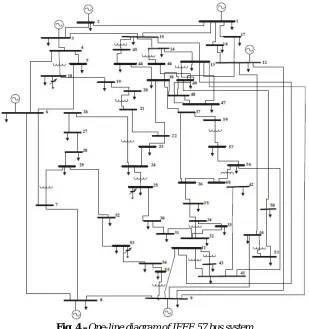
4.2.Results for IEEE 57 bus power system
In the following section, IEEE 57-bus system, whose single line diagram is as Fig. 4, is used in order to evaluate the efficacy of BOA. The data of this power system can be seen in [23]. ORPD problem for this system should be solved as a 25-dementional search space with 7 generator voltages, 15 transformer taps, and 3 reactive power sources.
T 3 6 0 . 9 5 8 0 0 . 9 6 0 0 0 0 0 . 9 6 0 0 0 0 . 9 9 0 0
C a p a c i t o r b a n k s
Q C - 1 0 5 . 0 0 0 0 3 . 2 0 0 0 0 0 3 . 6 0 0 0 0 4 . 8 0 0 0
Q C - 1 2 5 . 0 0 0 0 0 . 5 0 0 0 0 0 1 . 3 0 0 0 0 1 . 3 0 0 0
Q C - 1 5 5 . 0 0 0 0 4 . 9 0 0 0 0 0 2 . 7 0 0 0 0 4 . 5 0 0 0
Q C - 1 7 5 . 0 0 0 0 0 . 1 0 0 0 0 0 0 . 9 0 0 0 0 2 . 0 0 0 0
Q C - 2 0 5 . 0 0 0 0 3 . 8 0 0 0 0 0 4 . 2 0 0 0 0 4 . 3 0 0 0
Q C - 2 1 5 . 0 0 0 0 5 . 0 0 0 0 0 0 2 . 7 0 0 0 0 3 . 9 0 0 0
Q C - 2 3 5 . 0 0 0 0 5 . 0 0 0 0 0 0 3 . 0 0 0 0 0 4 0 0 0 0
Q C - 2 4 4 . 1 4 8 2 3 . 9 0 0 0 0 0 1 . 7 0 0 0 0 4 . 5 0 0 0
Q C - 2 9 0 . 7 0 6 9 1 . 5 0 0 0 0 0 1 . 8 0 0 0 0 3 . 4 0 0 0
PL o s s, M W 9 . 8 9 4 9 5 . 7 5 0 0 0 0 6 . 3 4 0 0 0 1 0 . 5 7 0
4.2.1. Active power loss Minimization
Table 3 shows the obtained results of power loss minimization in IEEE 57 bus power system. To reveal the superiority of the suggested strategy, in Table 3 BOA based results have been presented along with results of other optimizers including NGBWCA, WCA, OGSA and GSA.
Fig. 4 –One-line diagram of IEEE 57 bus system
From Table 3, it can be seen that BOA results realize optimal value of active power loss. Amongst the compared approaches, the best loss value was attained by the proposed strategy. The value of loss returned by BOA is 21.6380 MW. The best solutions obtained by different methods for this objective are presented in Table 3.
Table 3
Optimal parameter settings for loss minimization in IEEE 57 bus system
V a r i a b l e B O A N G B W C A W C A O G S A [ 1 7 ] G S A [ 4 7 ]
G e n e r a t o r v o l t a g e
V 1 1 . 1 0 0 0 1 . 0 6 0 0 1 . 0 6 0 5 1 . 0 6 0 0 1 . 0 6 0 0 0 0
V 2 1 . 1 0 0 0 1 . 0 5 9 1 1 . 0 6 0 2 1 . 0 5 9 4 1 . 0 6 0 0 0 0
V 3 1 . 0 4 6 5 1 . 0 4 9 2 1 . 0 4 9 7 1 . 0 4 9 2 1 . 0 6 0 0 0 0
V 8 1 . 1 0 0 0 1 . 0 5 8 6 1 . 0 6 0 0 1 . 0 6 0 0 1 . 0 5 4 9 5 5
V 9 1 . 0 9 1 2 1 . 0 4 6 1 1 . 0 5 8 9 1 . 0 4 5 0 1 . 0 0 9 8 0 1
V 1 2 1 . 0 9 2 6 1 . 0 4 1 3 1 . 0 5 3 8 1 . 0 4 0 7 1 . 0 1 8 5 9 1
T r a n s f o r m e r t a p r a t i o
T 4 – 1 8 0 . 9 1 2 5 0 . 9 7 1 2 0 . 9 9 2 3 0 . 9 0 0 0 1 . 1 0 0 0 0 0
T 4 – 1 8 0 . 9 0 1 2 0 . 9 2 4 3 0 . 9 8 1 4 0 . 9 9 4 7 1 . 0 8 2 6 3 4
T 2 1 – 2 0 0 . 9 5 3 5 0 . 9 1 2 3 0 . 9 3 5 4 0 . 9 0 0 0 0 . 9 2 1 9 8 7
T 2 4 – 2 6 1 . 0 0 2 3 0 . 9 0 0 1 0 . 9 9 5 3 0 . 9 0 0 1 1 . 0 1 6 7 3 1
T 7 – 2 9 1 . 0 0 5 6 0 . 9 1 1 2 0 . 9 9 6 3 0 . 9 1 1 1 0 . 9 9 6 2 6 2
T 3 4 – 3 2 1 . 0 1 5 0 0 . 9 0 0 4 0 . 9 7 1 2 0 . 9 0 0 0 1 . 1 0 0 0 0 0
T 1 1 – 4 1 1 . 0 2 6 6 0 . 9 1 2 8 0 . 9 8 6 5 0 . 9 0 0 0 1 . 0 7 4 6 2 5
T 1 5 – 4 5 0 . 9 8 1 7 0 . 9 0 0 0 0 . 9 2 4 5 0 . 9 0 0 0 0 . 9 5 4 3 4 0
T 1 4 – 4 6 0 . 9 8 3 8 1 . 0 2 1 8 1 . 0 3 4 5 1 . 0 4 6 4 0 . 9 3 7 7 2 2
T 1 0 – 5 1 0 . 9 8 0 3 0 . 9 9 0 2 1 . 0 0 5 6 0 . 9 8 7 5 1 . 0 1 6 7 9 0
T 1 3 – 4 9 0 . 9 6 2 0 0 . 9 5 6 8 0 . 9 8 2 5 0 . 9 6 3 8 1 . 0 5 2 5 7 2
T 1 1 – 4 3 1 . 0 2 1 8 0 . 9 0 0 0 0 . 9 7 1 5 0 . 9 0 0 0 1 . 1 0 0 0 0 0
T 4 0 – 5 6 1 . 0 1 5 0 0 . 9 0 0 0 0 . 9 9 2 3 0 . 9 0 0 0 0 . 9 7 9 9 9 2
T 3 9 – 5 7 1 . 1 0 0 0 1 . 0 1 1 8 1 . 0 1 8 6 1 . 0 1 4 8 1 . 0 2 4 6 5 3
T 9 – 5 5 1 . 0 2 3 8 1 . 0 0 0 0 1 . 0 0 2 4 0 . 9 8 3 0 1 . 0 3 7 3 1 6
C a p a c i t o r b a n k s
Q C - 1 8 0 0 . 0 9 1 4 0 . 0 9 8 8 0 . 0 6 8 2 0 . 0 7 8 2 5 4
Q C - 2 5 1 0 . 0 0 0 0 0 . 0 5 8 7 0 . 0 5 9 0 0 . 0 5 9 0 0 . 0 0 5 8 6 9 Q C - 5 3 6 . 9 9 5 6 0 . 0 6 3 4 0 . 0 6 2 9 0 . 0 6 3 0 0 . 0 4 6 8 7 2 PL o s s , p . u . 2 1 . 6 3 8 0 0 . 2 3 2 7 0 . 2 4 8 2 0 . 2 3 4 3 0 . 2 3 4 6 1 1 9 4
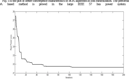
Fig. 5 is the plot of better convergence characteristics of BOA algorithm in loss minimization. The performance of BOA based method is proved in the large IEEE 57 bus power system here.
Fig. 5 –Convergence quality of BOA in loss minimization in IEEE 57 bus system
4.2.2. VD Minimization
In Table 4, the best solutions obtained by BOA for VD minimization have been tabulated along with the results of NGBWCA, WCA and OGSA algorithms. From this Table, it can be recognized that BOA outperforms other compared methods. The simulation outcomes of VD minimization indicate that the proposed BOA provides better solutions than other algorithms. The proposed method outperforms all the three other algorithms in bringing out best results for VD minimization.
Table 4
Optimal parameter settings for voltage deviation in IEEE 57 bus system
V a r i a b l e B O A N G B W C A W C A O G S A [ 1 7 ]
G e n e r a t o r v o l t a g e
V 1 0 . 9 7 7 0 1 . 0 1 5 1 1 . 0 2 4 2 1 . 0 1 3 8
V 2 1 . 0 7 9 5 0 . 9 8 1 0 0 . 9 9 5 3 0 . 9 6 0 8
V 3 0 . 9 7 5 7 1 . 0 0 0 2 1 . 0 0 9 8 1 . 0 1 7 3
V 6 0 . 9 8 7 9 1 . 0 0 3 9 1 . 0 1 7 6 0 . 9 8 9 8
V 8 1 . 0 4 4 0 1 . 0 1 9 8 1 . 0 2 6 8 1 . 0 3 6 2
V 1 2 1 . 0 4 3 8 1 . 0 0 8 1 1 . 0 1 2 5 1 . 0 1 3 6
T r a n s f o r m e r t a p r a t i o
T 4 – 1 8 0 . 9 4 3 6 1 . 0 1 8 5 1 . 0 2 1 7 0 . 9 8 3 3
T 4 – 1 8 1 . 0 0 7 6 0 . 9 6 0 1 0 . 9 6 1 4 0 . 9 5 0 3
T 2 1 – 2 0 0 . 9 6 4 7 0 . 9 4 5 8 0 . 9 4 9 6 0 . 9 5 2 3
T 2 4 – 2 6 0 . 9 9 4 4 0 . 9 9 1 9 0 . 9 9 0 1 1 . 0 0 3 6
T 7 – 2 9 0 . 9 7 5 5 0 . 9 9 5 1 0 . 9 9 8 6 0 . 9 7 7 8
T 3 4 – 3 2 0 . 9 2 2 4 0 . 9 0 0 0 0 . 9 0 0 0 0 . 9 1 4 6
T 1 1 – 4 1 0 . 9 0 0 0 0 . 9 6 2 2 0 . 9 6 3 4 0 . 9 4 5 4
T 1 5 – 4 5 0 . 9 5 5 8 0 . 9 0 5 8 0 . 9 0 6 3 0 . 9 2 6 5
T 1 4 – 4 6 0 . 9 8 2 2 0 . 9 7 6 4 0 . 9 8 0 1 0 . 9 9 6 0
T 1 0 – 5 1 1 . 0 0 8 9 1 . 0 6 0 0 1 . 0 6 3 1 1 . 0 3 8 6
T 1 3 – 4 9 0 . 9 0 2 0 0 . 9 1 0 0 0 . 9 1 3 1 0 . 9 0 6 0
T 1 1 – 4 3 0 . 9 8 4 5 0 . 9 3 0 2 0 . 9 2 9 4 0 . 9 2 3 4
T 4 0 – 5 6 1 . 0 3 5 0 0 . 9 7 7 0 0 . 9 7 8 2 0 . 9 8 7 1
T 3 9 – 5 7 1 . 0 4 2 4 1 . 0 2 7 1 1 . 0 2 8 6 1 . 0 1 3 2
T 9 – 5 5 0 . 9 9 7 4 0 . 9 0 0 0 0 . 9 0 5 3 0 . 9 3 7 2
C a p a c i t o r b a n k s
Q C - 1 8 9 . 9 8 4 1 0 . 0 5 5 0 0 . 0 5 9 3 0 . 0 4 6 3
Q C - 2 5 9 . 9 6 8 6 0 . 0 5 9 0 0 . 0 5 9 1 0 . 0 5 9 0
Q C - 5 3 9 . 9 7 7 3 0 . 0 3 8 1 0 . 0 3 8 2 0 . 0 6 2 8
P L o s s , p . u . 4 2 . 6 2 2 9 0 . 2 9 2 0 0 . 3 0 0 2 0 . 3 2 3 4
T V D , p . u . 0 . 6 3 3 3 0 . 6 5 0 1 0 . 6 6 3 1 0 . 6 9 8 2
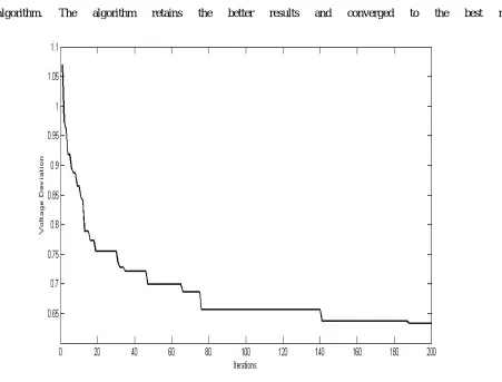
algorithm. The algorithm retains the better results and converged to the best results.
Fig. 6 –Convergence quality of BOA in voltage deviation in IEEE 57 bus system
V. CONCLUSIONS
In this work, the BOA algorithm is implemented in ORPD with two objectives. The efficiency of the proposed BOA is tested on IEEE-30 and IEEE-57 bus power systems. The experimental results and statistical data clearly demonstrate the efficiency of the BOA algorithm in solving ORPD problems. The strength of the proposed algorithm is proved in both the challenging tasks in ORPD problem.
The algorithm is efficient and easy to be implemented for engineering optimizations. Hybridization of the proposed BOA with other well-established metaheuristic optimisation algorithms may be tried for improved performance. Use of recently developed metaheuristic algorithms is recommended for ORPD problem.
REFERENCES
[1] Sun, D.I., Ashley, B., Brewer, B., Hughes, A. and Tinney, W.F., 1984. Optimal power flow by Newton approach. IEEE Transactions on Power
Apparatus and systems, (10), pp.2864-2880.
[3] Ghasemi, M., Ghavidel, S., Rahmani, S., Roosta, A. and Falah, H., 2014. A novel hybrid algorithm of imperialist competitive algorithm and teaching learning algorithm for optimal power flow problem with non-smooth cost functions. Engineering Applications of Artificial Intelligence, 29, pp.54-69.
[4] Adaryani, M.R. and Karami, A., 2013. Artificial bee colony algorithm for solving multi-objective optimal power flow problem. International Journal of Electrical Power & Energy Systems, 53, pp.219-230.
[5] Ghasemi, M., Ghavidel, S., Akbari, E. and Vahed, A.A., 2014. Solving non-linear, non-smooth and non-convex optimal power flow problems using chaotic invasive weed optimization algorithms based on chaos. Energy, 73, pp.340-353.
[6] Shaheen, A.M., El-Sehiemy, R.A. and Farrag, S.M., 2016. Solving multi-objective optimal power flow problem via forced initialised differential evolution algorithm. IET Generation, Transmission & Distribution, 10(7), pp.1634-1647.
[7] Berizzi, A., Bovo, C., Merlo, M. and Delfanti, M., 2012. A ga approach to compare orpf objective functions including secondary voltage regulation. Electric Power Systems Research, 84(1), pp.187-194.
[8] Tuo, S., Yong, L. and Zhou, T., 2013. An improved harmony search based on teaching-learning strategy for unconstrained optimization problems. Mathematical Problems in Engineering, 2013.
[9] Roy, P.K., Paul, C. and Sultana, S., 2014. Oppositional teaching learning based optimization approach for combined heat and power dispatch. International Journal of Electrical Power & Energy Systems, 57, pp.392-403.
[10] Berizzi, A., Bovo, C., Merlo, M. and Delfanti, M., 2012. A ga approach to compare orpf objective functions including secondary voltage regulation. Electric Power Systems Research, 84(1), pp.187-194.
[11] Berizzi, A., Bovo, C., Merlo, M. and Delfanti, M., 2012. A ga approach to compare orpf objective functions including secondary voltage regulation. Electric Power Systems Research, 84(1), pp.187-194.
[12] Ghasemi, M., Ghavidel, S., Ghanbarian, M.M., Gharibzadeh, M. and Vahed, A.A., 2014. Multi-objective optimal power flow considering the cost, emission, voltage deviation and power losses using multi-objective modified imperialist competitive algorithm. Energy, 78, pp.276-289. [13] Vaisakh, K. and Rao, P.K., 2008, December. Optimal reactive power allocation using PSO-DV hybrid algorithm. In India Conference, 2008.
INDICON 2008. Annual IEEE (Vol. 1, pp. 246-251). IEEE.
[14] Liang, C.H., Chung, C.Y., Wong, K.P., Duan, X.Z. and Tse, C.T., 2007. Study of differential evolution for optimal reactive power flow. IET generation, transmission & distribution, 1(2), pp.253-260.
[15] Gatterbauer, W., 2010. Economic efficiency of decentralized unit commitment from a generator’s perspective. Engineering Electricity Services of the Future. Springer, p.16.
[16] Dai, C., Chen, W., Zhu, Y. and Zhang, X., 2009. Reactive power dispatch considering voltage stability with seeker optimization algorithm.
Electric Power Systems Research, 79(10), pp.1462-1471.
[17] Duman, S., Sonmez, Y., Guvenc, U. and Yorukeren, N., 2012. Optimal reactive power dispatch using a gravitational search algorithm. IET generation, transmission & distribution, 6(6), pp.563-576.
[18] Saraswat, A. and Saini, A., 2013. Multi-objective optimal reactive power dispatch considering voltage stability in power systems using HFMOEA. Engineering Applications of Artificial Intelligence, 26(1), pp.390-404.
[19] Kumar, A.R. and Premalatha, L., 2015. Optimal power flow for a deregulated power system using adaptive real coded biogeography-based optimization. International Journal of Electrical Power & Energy Systems, 73, pp.393-399.
[20] Bouchekara, H.R.E.H., Abido, M.A. and Boucherma, M., 2014. Optimal power flow using teaching-learning-based optimization technique.
Electric Power Systems Research, 114, pp.49-59.
[21] Yang, X.S. and Hossein Gandomi, A., 2012. Bat algorithm: a novel approach for global engineering optimization. Engineering Computations, 29(5), pp.464-483.
[22] Gandomi, A.H., Yang, X.S., Alavi, A.H. and Talatahari, S., 2013. Bat algorithm for constrained optimization tasks. Neural Computing and Applications, 22(6), pp.1239-1255.
[23] Heidari, A.A., Abbaspour, R.A. and Jordehi, A.R., 2017. Gaussian bare-bones water cycle algorithm for optimal reactive power dispatch in electrical power systems. Applied Soft Computing, 57, pp.657-671.
[24] Rajan, A. and Malakar, T., 2015. Optimal reactive power dispatch using hybrid Nelder–Mead simplex based firefly algorithm. International Journal of Electrical Power & Energy Systems, 66, pp.9-24.
[25] Mandal, B. and Roy, P.K., 2013. Optimal reactive power dispatch using quasi-oppositional teaching learning based optimization. International Journal of Electrical Power & Energy Systems, 53, pp.123-134.
[26] Bhattacharya, A. and Chattopadhyay, P.K., 2010. Solution of optimal reactive power flow using biogeography-based optimization.
International Journal of Electrical and Electronics Engineering, 4(8), pp.568-576.
[27] Shaw, B., Mukherjee, V. and Ghoshal, S.P., 2014. Solution of reactive power dispatch of power systems by an opposition-based gravitational search algorithm. International Journal of Electrical Power & Energy Systems, 55, pp.29-40.