Analog Circuit Synthesis Using PSO and HPSO Algorithm

(1)

Analog Circuit Synthesis Using PSO and

HPSO Algorithm

Bhoomi N. Thakkar1, Vimal H. Nayak2

PG Student [ECE], Dept. of ECE, Silver Oak College of Engineering and Technology, Ahmedabad, Gujarat, India1

Assistant Professor, Dept. of ECE, Silver Oak College of Engineering and Technology, Ahmedabad, Gujarat, India2

ABSTRACT: In this paper, PSO Algorithm and HPSO Algorithm are used for the optimization of RC Filter and the results of both the algorithms are compared. By using these algorithms on sphere and rosenbrock benchmark functionsthe best values of RC filter parameters are achieved in such a way that it minimizes error between simulated output and optimized output. With the help of this parameters the circuit simulatorgives the cut off frequency (1.000000e + 03) which is much closer to the standard cut off frequency i.e.1k.

KEYWORDS: Automatic Analog Circuit Design, Analog Circuit Synthesis, Hierarchical Particle Swarm Optimization, Particle Swarm Optimization.

I. INTRODUCTION

Technology scaling, high performance demands, and system-on-chip applications force analog modules to be implemented in the same technology nodes as that of digital circuits or at most few nodes behind digital technology nodes.As technology is scaled down, the physical models of analog circuits have become complex due to various short-channel effects. These factors have led to the manual design of analog circuits to be a challenging and timewasting task and hence efficient automatic design techniques are required.There are various optimization techniques have been reported previously for automatic design of analog circuits. The classical optimization methods need to calculate derivatives and require good initial guess for the design variables. In the absence of first guess close to the globally optimum solution, these algorithms would generally stick at a locally optimum solution. The evolutionary algorithms, which can be used to solve multimodal optimization problems, do not suffer from problems associated with the gradient-based methods. The Genetic Algorithm (GA), developed by Holland. Particle swarm optimization (PSO), another evolutionary algorithm, was proposed by Kennedy and Eberhart. It is reported in literature that while increasing particle number in PSO improves the performance. The hierarchical PSO algorithm, a recent variant of PSO algorithm, has been explored for automatic analog circuit design applications.

In this paper, we propose and demonstrate the PSO algorithm and a hierarchical PSO algorithm (HPSO) are proposed for automatic analog circuit design. In this paper, the RC filter is considered as a design problem. The design results obtained with the PSO algorithm and HPSO algorithm on two benchmark functions and are also compared with each other. It is shown that the results are almost same.

II. PSO ALGORITHM AND ITS IMPLEMENTATION

(2)

ISSN (Online): 2278 – 8875

I

nternational

J

ournal of

A

dvanced

R

esearch in

E

lectrical,

E

lectronics and

I

nstrumentation

E

ngineering

(An ISO 3297: 2007 Certified Organization)

Vol. 5, Issue 3, March 2016

experience of others round them (global search) [1].

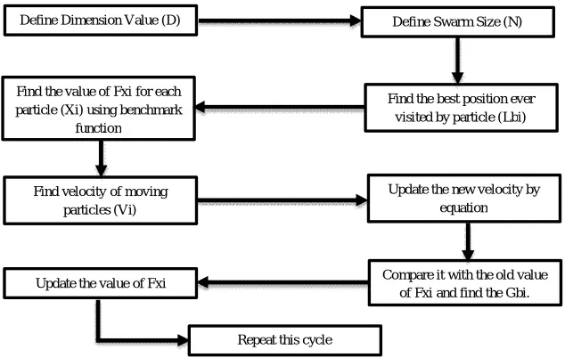
Figure 1: Flow Chart of PSO Algorithm

The Flow Chart of Implementation of PSO algorithm is shown inFigure 1. The process is initialized with a group of random particles N. The ith particle is represented by its position as a point in a D-dimensional space, where D is the number of variables. During the process, each particle i monitors three values: its current position (Xi); the best position ever visited by particle (Lbi); velocity of a moving particle (Vi).

In each time interval (cycle), the global best position (gbi) of a particle is calculated as the best fitness of all particles. Accordingly, each particle updates its velocity Vi to catch up with the best particle g.

New Vi = WVi + C1R1(Lbi – Xi) + C2R2(Gbi – Xi) Eq. (1)

As such, using the new velocity Vi, the particle’s updated position becomes:

New position Xi =current position Xi + New Vi; Eq. (2)

Table 1: Control Parameters of PSO Algorithm

Control Parameters Values

Dimension(D) 30

Swarm size 75

Femax 2E5

Weighting factor, Wh 0.9

Weighting factor, Wl 0.4

Where, Vmax ≥ Vi ≥ -Vmax and c1, c2 are two positive constants named learning factors (usually c1=c2=2). rand( ) and Rand( ) are two random functions in the range [0, 1], Vmax is an upper limit on the maximum change of particle velocity and w is the weighting factor. It is noted that the second term in Eq. (1) represents cognition, or the private thinking of the particle when comparing its existing position to its own best. The third term in Eq. (1), on the other hand, represents the social cooperation among the particles, which compares a particle’s current position to that of the best particle. Also, to control the change of particle’s velocities, upper and lower bounds for velocity change is limited to a user-specified value of max. Once the new position of a particle is calculated using Eq. (2), the particle, then, flies towards it [1].

Define Dimension Value (D) Define Swarm Size (N)

Find the value of Fxi for each particle (Xi) using benchmark

function

Find the best position ever visited by particle (Lbi)

Find velocity of moving particles (Vi)

Update the new velocity by equation

Update the value of Fxi Compare it with the old value

of Fxi and find the Gbi.

(3)

In this paper two benchmark functions are used i.e. sphere and rosenbrock. The equations of these benchmark functions are, Sphere Benchmark function is [2],

∑i=0 to D (Xi2), where N = 30 Eq. (3) Rosenbrock benchmark Function is [2],

∑i=0 to D-1 {100 (Xi2 – Xi+1)2 + (1 – xi2)} Eq. (4)

Result of PSO algorithm on above two benchmark functions are as shown in below Figures.

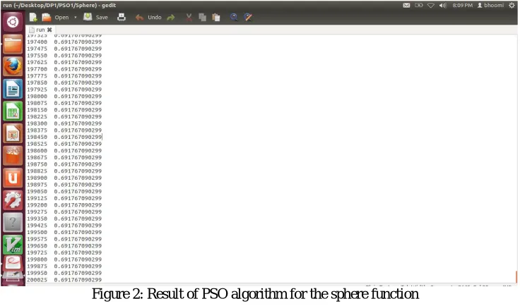
Figure 2: Result of PSO algorithm for the sphere function

As shown in Figure 2 the mean value of sphere function is 0.691767090299 for PSO algorithm.

Figure 3: Result of PSO algorithm for the Rosenbrock function

(4)

ISSN (Online): 2278 – 8875

I

nternational

J

ournal of

A

dvanced

R

esearch in

E

lectrical,

E

lectronics and

I

nstrumentation

E

ngineering

III. HPSO ALGORITHM AND THEIR IMPLEMENTATION

In the HPSO algorithm, the particles are divided into many groups with each group having a “local leader” and particles within a group follow their local leader. This feature of the HPSO algorithm enables enhanced exploration of the search space and shows better consistency in finding the optimum solution. The organization of particles in HPSO is described below. The organization of particles in HPSO is described below. Let us assume that the total number of particles is N. In HPSO, these particles are first arranged in ascending order according to their fitness, with the globally best particle (the “global leader”) at position N, as shown in below Figure 4.The next M best particles are designated as the “local leaders.” The remaining (N −M −1) particles are divided into M groups. The M local leaders are assigned to the M groups as shown in Figure 4.

Figure 4: Arrangement of particles in the HPSO algorithm [1].

The common particles follow their local leader and the local leaders follow the global leader. Any particle is permissible to become a local leader or the global leader, depending upon its fitness relative to the other particles [1].

Result of HPSO algorithm on two benchmark functions are as shown in below Figures.

(5)

As shown in Figure 5 shows that the mean value of sphere function is 1.04290779626 for HPSO algorithm.

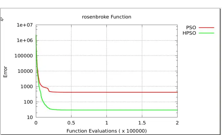
Figure 6: Result of HPSO algorithm for the Rosenbrock function

And from Figure 6 shows that the mean value of rosenbrock function is 29.8275602641 for HPSO algorithm.

IV. COMPARISION OF PSO AND HPSO ALGORITHM

In above section II and III implementation of PSO and HPSO algorithm is done. By using their mean valuesthe comparison graphs of error versus function evolutions for sphere and rosenbrock function can be plot which is in the below Figures.In these graphs the inaccuracy will be reduceas increasing in the function evolutions.

(6)

ISSN (Online): 2278 – 8875

I

nternational

J

ournal of

A

dvanced

R

esearch in

E

lectrical,

E

lectronics and

I

nstrumentation

E

ngineering

Figure 8: Comparison between PSO and HPSO for rosenbrock function

In the above graphs red line shows PSO algorithm and Green shows HPSO algorithm. For sphere function the result of PSO and HPSO algorithms are almost same as shown in Figure 7. But for the rosenbrock function HPSO algorithm gives better result than the PSO algorithm as shown in Figure 8.

V. AUTOMATIC ANALOG CIRCUIT DESIGN SETUP

During circuit design, a circuit simulator is linked with the optimizer module and the desired specifications are provided as input. The optimizer module (PSO Algorithm or HPSO Algorithm) provides values for design variables to circuit simulator and calculates the error between desired performance measures and simulator returned performance measures. The optimizer module updates the design variables using a suitable optimization algorithm to minimize the error.

Figure 9: Block diagram of automatic analog circuit design

In this paper, the error function is defined as,

(7)

Where, SpecDesired represents desired performance measures (lower or upper limit as applicable) and SpecSim denotes the performance measures returned by a circuit simulator for a particular solution provided by the optimizer. In each circuit design evolution, those performance measures which satisfy the conditions given in Eq. (1), will not contribute to the error function in Eq. (5).

With the above procedure automatic design of any analog circuit can be done. In this paper the low pass filter which has only two parameters i.e. R1 & C1, is designed with the help of PSO and HPSO algorithm.Parameters values and their ranges which are given to the PSO and HPSO algorithms for obtaining desired output are as listed in Table 2.

Table 2: Parameters values given to the both algorithms for LPF

Design variables Values

Dimension(N) 2

Swarm size 10

Cutoff frequency which we want to obtained 1E3

Range of the R1 1e3 – 0.0E-6

Range of C1 100e3 – 0.01E-6

The best values of design parameters obtained with the help of PSO and HPSO algorithm to get the best low pass filter characteristics with the Cut off frequency 1k i.e.,

Table 3: Obtained Values of R1 and C1

Algorithm Obtained Value of R1 Obtained Value of C1

PSO 1737.03676004 9.1407064377e – 08

HPSO 15877.7407888 1e – 08

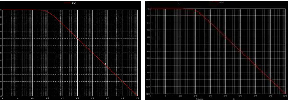
By using this parameters we are achieving the cut off frequency 1.000000e + 03, which is very close to standard cut off frequency value i.e.1k and by using this obtained Cut off frequency we can plot the graph of the characteristic of the Low pass filter which is shown in Figure 10a and Figure 10b.

(8)

ISSN (Online): 2278 – 8875

I

nternational

J

ournal of

A

dvanced

R

esearch in

E

lectrical,

E

lectronics and

I

nstrumentation

E

ngineering

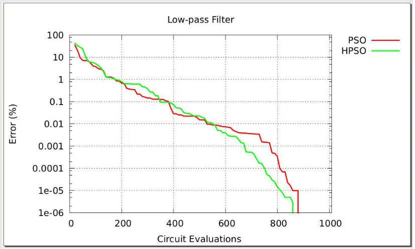
With the help of above results comparison of PSO and HPSO algorithm for low pass filter is plotted for the error versus circuit evaluations. The result of PSO and HPSO algorithms are almost same which is shown in Figure 11.

Figure 11: Graph of the comparison of PSO and HPSO for LPF

VI. CONCLUSION

In this paper, detailed analysis and implementation of PSO and HPSO Algorithm is proposed for the optimization problem of Automatic Analog Circuit Design. First PSO and HPSO algorithm is tested over two classical Benchmark functions. Low pass filter as benchmark circuit is taken as design example. The obtained design variables are close in performance. In the case of Low pass filter, it gives the cut off frequency (1.000000e + 03) which is much closer to the standard cut off frequency i.e.1k with respect to PSO and HPSO algorithm.By comparing results of PSO and HPSO algorithm it is shown that the results are almost same for both the algorithms.

REFERENCES

[1] Rajesh A. Thakker, M. Shojaei Baghini, and M. B. Patil, “Automatic Design of Low-Power, Low-Voltage Analog Circuits Using Particle Swarm Optimization with Re-Initialization.” Journal of low power electronics, vol. 5, pp.1-12, 2009.

[2] Dervis Karaboga and Bahriye Basturk, “A powerful and efficient algorithm for numerical function optimization: artificial bee colony (ABC) algorithm.” J Glob Optim”, vol. 39, pp.459471, 2007.

[3] Revna Acar Vural, Student Member, IEEE, Tulay Yildirim, Member, IEEE, Tevfik Kadioglu, and Aysen Basargan, “Performance Evaluation of Evolutionary Algorithms for Optimal Filter Design”,IEEE, vol. 16, , Issue no. 1, pp.135-147, 2012.