A Low Complexity 8 × 8 DCT Transform for
Image Compression
Parvin Tamboli1, Aparna Shinde2
PG Student [VLSI & ES] , Dept. of E&TC, D.Y. Patil College of Engineering, Akurdi, Pune, Maharashtra,, India1 Assistant Professor, Dept. of E&TC, D.Y.Patil College of Engineering, Akurdi, Pune, Maharashtra, India2
ABSTRACT: In this paper, an orthogonal 8×8 orthogonal transform matrix suitable for image compression is proposed. An algorithm for its fast computation is developed. The proposed transform requires 14 additions only. The proposed transform possesses low computational complexity and is compared to state-of-the-art DCT approximations in terms of both algorithm complexity and peak signal-to-noise ratio. Such approximations can be realized in digital VLSI hardware using additions and subtractions only. This gives significant reduction in chip area.
KEYWORDS: Approximate DCT, Image Compression, Fast algorithm, Low complexity transform
I.INTRODUCTION
The recent mobile and communication system require very fast compression. The floating point discrete cosine transform (DCT) which is well known in image compression can not meet the requirements of fast computation. The floating-point operations are expensive in terms of circuitry complexity and power consumption. Therefore, minimizing the number of floating-point operations is an essential property in a fast algorithm. One way of solving this issue is by means of approximate transforms. Therefore there has been a huge interest is created in developing
integer and multiplication-free transforms.
The signal processing community turned its focus to approximate algorithms for the computation of the 8-point DCT. While not computing the DCT exactly, approximate methods can provide meaningful estimations at low-complexity requirements. The prominent approximate DCT methods include include the Bouguezel-Ahmad-Swamy (BAS) series of algorithms [2],[3] and the Cintra-Bayer (CB) approximate DCT [4]. In this context, the aim of this paper is to introduce a new low-complexity DCT approximation for image compression which requires 14 additions only.
II.RELATED WORK
In this section, the important DCT approximate methods are explained in terms of its transformation matrices and the associated fast algorithms obtained by matrix factorization techniques.
1. Bouguezel-Ahmad-Swamy Approximate DCT
In [2], a low-complexity approximate was introduced by Bouguezel et al. This approximate DCT is known as BAS- 2008 approximation. The BAS-2008 approximation has the following mathematical structure.
C = D · T
The diagonal matrix D is given as
D = diag ( 1/√8, 1/√4, 1/√5, 1/√2, 1/√8, 1/√4, 1/√5, 1/√2 ) And the transformation matrix is
= D ·
⎣ ⎢ ⎢ ⎢ ⎢ ⎢ ⎢
⎡ 11 11 10 10 10 10 −11 −11
1 1/2 −1/2 −1 −1 −1/2 1/2 1
0 0 −1 0 0 1 0 0
1 −1 −1 1 1 −1 −1 1
1 −1 0 0 0 0 1 −1
1/2 −1 1 −1/2 −1/2 1 −1 1/2
0 0 0 −1 1 0 0 0 ⎦
A fast algorithm for matrix T is given as, T = A3 · A2 · A1
Where,
A
1=⎣ ⎢ ⎢ ⎢ ⎢ ⎢ ⎢
⎡1 0 0 00 1 0 0 00 00 01 10
0 0 1 0 0 1 0 0
0 0 0 1 1 0 0 0
0 0 0 1 ˗1 0 0 0
0 0 1 0 0 ˗1 0 0
0 1 0 0 0 0 ˗1 0
1 0 0 0 0 0 0 ˗1⎦
⎥ ⎥ ⎥ ⎥ ⎥ ⎥ ⎤
A2 =
⎣ ⎢ ⎢ ⎢ ⎢ ⎢ ⎢
⎡1 00 0 00 10 00 00 01 01
0 1 1 0 0 0 0 0
0 0 0 0 0 −1 0 0
0 1 −1 0 0 0 0 0
0 0 0 0 0 0 −1 1
1 0 0 −1 0 0 0 0
0 0 0 0 −1 0 0 0⎦
⎥ ⎥ ⎥ ⎥ ⎥ ⎥ ⎤
A3 =
⎣ ⎢ ⎢ ⎢ ⎢ ⎢ ⎢
⎡1 00 1 10 00 00 00 00 00
0 0 0 0 1/2 0 1 0
0 0 0 1 0 0 0 0
1 0 −1 0 0 0 0 0
0 0 0 0 0 1 0 0
0 0 0 0 −1 0 1/2 0
0 0 0 0 0 0 0 1⎦
⎥ ⎥ ⎥ ⎥ ⎥ ⎥ ⎤
2. CB 2011 Approximation
By means of rounding off the elements of the exact DCT matrix, a DCT approximation is obtained and described in [4]. The transformation matrix is given as
C = D · T
= D ·
⎣ ⎢ ⎢ ⎢ ⎢ ⎢ ⎢
⎡11 11 11 10 10 −11 −11 −11
1 0 0 −1 −1 0 0 1
1 0 −1 −1 1 1 0 −1
1 −1 −1 1 1 −1 −1 1
1 −1 0 1 −1 0 1 −1
0 −1 1 0 0 1 −1 0
0 −1 1 −1 1 −1 1 0 ⎦
⎥ ⎥ ⎥ ⎥ ⎥ ⎥ ⎤
And diagonal matrix D = diag (1/√8, 1/√6, ½, 1/√6, 1/√8, 1/√6, ½, 1/√6 )
The fast algorithm for T is given as T = P2 · A6 · A5 ·A1
A5 = diag (
1 0 0 1
0 1 1 0
0 1 −1 0
1 0 0 −1
·
−1 1 −1 0
−1 −1 0 1
1 0 −1 1
0 1 1 1
)
A6 = diag (1 1
1 −1 , -1, I5 )
And P4 is the permutation of ( 1) (2 5 8) (3 7 6 4 )
III. PROPOSED TRANSFORM
In this section, we propose a multiplication-free transform suitable for image compression. We also develop an efficient algorithm for fast computation of the proposed transform. The proposed DCT approximation is given as
C = D · T
Where T is transformation matrix and it is given as
T = ⎣ ⎢ ⎢ ⎢ ⎢ ⎢ ⎢
⎡11 ˗11 ˗11 11 11 ˗11 ˗11 11
0 0 0 1 ˗1 0 0 0
0 0 1 0 0 ˗1 0 0
1 0 0 0 0 0 0 ˗1
1 0 0 ˗1 ˗1 0 0 1
0 ˗1 1 0 0 1 ˗1 0
0 1 0 0 0 0 ˗1 0⎦
⎥ ⎥ ⎥ ⎥ ⎥ ⎥ ⎤
And the diagonal matrix D is given as
D = diag ( 1/√8, 1/√2, ½, 1/√2, 1/√8, 1/√2, ½, 1/√2 )
The transformation matrix T has entries in {0, ±1} and it can be given a sparse factorization according to
T = P4 · A12 · A11 · A1
Where
A
11= diag (
1
0
0
1
0
1
1
0
0
1
˗
1
0
1
0
0
˗
1
, I
4)
A12 = diag ( 11 1
˗1 , ˗1, I5 )
A
1=⎣ ⎢ ⎢ ⎢ ⎢ ⎢ ⎢
⎡1 0 0 00 1 0 0 00 00 01 10
0 0 1 0 0 1 0 0
0 0 0 1 1 0 0 0
0 0 0 1 ˗1 0 0 0
0 0 1 0 0 ˗1 0 0
0 1 0 0 0 0 ˗1 0
1 0 0 0 0 0 0 ˗1⎦
⎥ ⎥ ⎥ ⎥ ⎥ ⎥ ⎤
IV.EXPERIMENTAL RESULTS
The proposed algorithm is implemented in VHDL. In order to check the effectiveness of the proposed 8x8 transform, the experiments were performed involving test image. The results were evaluated for grayscale 256 ×256 pixel ‘Lena’ image, as shown in figure 1. The performance evaluation parameters under consideration are Mean Square Error (MSE) and Peak Signal to Noise Ratio (PSNR).
The MSE and PSNR are defined as
MSE = ∑ ∑ (Ai, j – Bi, j )2
where, A = Original image of size M × N
B = Reconstructed image of size M × N
PSNR = 10 log10 I2 ⁄ MSE
where, I is allowable image pixel intensity level. For 8 bit per pixel image,
I= 28 -1 =255
Figure 1: Experimental Image ‘ Lena’ 256 × 256
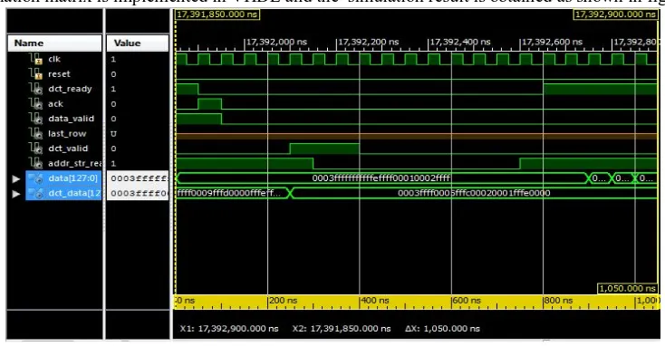
The transformation matrix is implemented in VHDL and the simulation result is obtained as shown in figure 2.
Figure 3 shows the compression results at different compression ratio with PSNR =27.208 dB
( a ) ( b ) ( c )
Figure 3 : ( a ) DCT Transformed Image , ( b ), ( c ) Quantized Images with quantization ratio of 50.65 % and
60.41 % resp. with PSNR 27. 208 dB
IV.PERFORMANCE EVALUATION
The table 1 gives comparative analysis of various DCT approximation methods.
Sr. No. Method Required Shift
operations
Required Addition
operations
PSNR (dB)
1 BAS 2011 [3] No 16 26.918
2 CB 2011 [4] No 22 27.369
3 App. DCT in [5] 2 14 27.820
4 App. DCT in [1] No 14 25.726
5 Proposed Transform No 14 27.208
Table 1: PSNR and Arithmetic Complexity Analysis of various DCT approximate methods
V. CONCLUSION
The proposed low-power 8-point DCT approximation method requires only 14 addition operations for implementation. The hardware architecture for the proposed transform is implemented in VHDL. The proposed transform offers low arithmetic complexity. The Table 1 indicates that the proposed transform provides good PSNR as compared wih same arithmetic complexity DCT method[1].
REFERENCES
[1] Uma Sadhvi Potluri, Arjuna Madanayake, Renato J. Cintra, Fbio M. Bayer,Sunera Kulasekera and Amila Edirisuriya, “ Improved 8-Point
Approximate DCT for Image and Video Compression Requiring Only 14 Additions ", IEEE Transactions on Circuits and Systems I: Regular Papers, vol. 61, no. 6, 2014.
[2] S. Bouguezel, M. O. Ahmad, and M. N. S. Swamy, “A novel transform for image compression,” in Proc. 53rd IEEE Int Midwest Symp.
Circuits System(MWSCAS), Aug. 2010, pp. 509–512.
[3] S. Bouguezel, M. O. Ahmad, and M. N. S. Swamy, “A low-complexity parametric transform for image compression,” in Proc. ISCAS, May
2011, pp. 2145–2148.
[4] R. J. Cintra and F. M. Bayer, “A DCT approximation for image compression, IEEE Signal Processing Lett., vol. 18 no
[5] Ranjan K. Senapati, Umesh C. Pati and Kamala K. Mahapatra, “A Low Complexity Orthogonal 8 × 8 Transform Matrix for Fast Image Compression,” Annual IEEE India Conference (INDICON), 2010, pp. 1-4
[6] Dariusz Puchala1 and Kamil Stokfiszewski, “ Low-Complexity Approximation of 8- point Discrete Cosine Transform for Image
Compression, ”Journal of Applied Computer Science, vol.20 no. 2, 2012, pp. 107-117
[7] N. Ahmed, T. Natarajan, and K. Rao, “Discrete Cosine Transfom,” Computers, IEEE Transactions on, vol. C-23, no. 1, Jan 1974, pp.90-93