An Efficient Algorithm for Power Load Flow
Solutions by Schur Complement and
Threshold Technique
Ahmed Al Ameri
1, Cristian Nichita
2and Brayima Dakyo
3Ph. D. Student; GREAH Lab., Le Havre Université, Le Havre, France1 Professor, GREAH Lab., Le Havre Université, Le Havre, France2 Professor, GREAH Lab., Le Havre Université, Le Havre, France3
ABSTRACT: This paper deals with a algorithm developed for load flow problems in electrical power systems.
Jacobian matrix in Newton Raphson method require large computer memory and take more computation time in calculations. Schur complement method can be reduce memory required by divided Jacobian matrix into two separated matrices with reasonable computation time. The proposed algorithm used this method with threshold technique in order to test different power systems. Results has been compared with Newton Raphson method and Fast Decoupled method in term of influence of convergence properties and algorithm efficiency.
KEYWORDS: Power system network, Load flow, Element incidence matrix, Schur complement method, Software
Development.
I.INTRODUCTION
P
ower flow analysis is necessary for planning, operation, economic scheduling and exchange of power between utilities. Power flow analysis is required for many other analyses such as transient stability, optimal power flow and contingency studies. The principal information of power flow analysis is to find the magnitude and phase angle of voltage at each bus and the real and reactive power flowing in each transmission lines. Power flow problem could be viewed as a multi-input multi-output system. Each input could have effect on each of the outputs, more or less. Thus it makes it more difficult to appreciate the correlation between these variables.In view of the topological specialty of transmission and distribution networks, many researchers has proposed several special load flow techniques [1-4]. However, an acceptable load flow method should meet the requirements such as high speed and low storage requirements, highly reliable, and accepted versatility and simplicity. The starting of studies for the load flow calculations was begin with the Ward & Hale [1] , while the Newton-Raphson (N-R) method [2], [3] are being widely used. The problem of the computation iteration time has been solved by the developments of the Fast Decoupled Load Flow [4], then Fast Load Flow Method Retaining Nonlinearity [5], and so on. A large variety of proposed solution for power flow problem addressing with different targets like reduce computation time [6-9], ill-conditioned cases and robustness [10–12], and optimal power flow (OPF) problems [10-15].
II. LOAD FLOW FOR POWER SYSTEM
This method requires the construction of admittance (n x n) matrix, where n is number of bus system. The diagonal elements of the admittance matrix represent the self-admittance of the bus and the off diagonal represent the mutual admittance between buses.
Y =
Y11 … Yjk
⋮ ⋱ ⋮
Ykj … Ykk
……….……… (1)
The real and reactive power calculated at specific bus using initial guess and specified voltage magnitude and angle. The iteration methods were used to solve this non linear equations like (Gauss Sidle and Newton Raphson). Newton Raphson was more efficient and robust and basically it calculated powers as follows[16]:
Pkcalc (x)= nj=1 Vk Vj |Ykj|cos(Ɵkj− δk+ δj) ……….……… (2)
Qcalc (x)k = − nj=1 Vk Vj |Ykj|sin(Ɵkj − δk+ δj) ……….……… (3)
Finalized the iteration will depend on tolerance of the power mismatch which calculated by their formulae
:
△ Pk(x) = Pksch − Pk calc (x)
……….……… (4)
△ Qk(x)= Qksch − Q k calc (x)
……….………(5)
The Jacobian matrix of this method can be represented by:
△ P
△ Q = J1 J2
J3 J4
△ δ
△ V ……….………(6)
The elements of the Jacobian matrix are partial derivative values of either P or Q with respect to either |V| or δ.
J =
∂P ∂δ
∂P ∂|V| ∂Q ∂δ
∂Q ∂|V|
….………(7)
Typically, the Jacobian matrix is inversed and added to the left side of the equation, the final form looks like the following:
△ δ △ V =
J1 J2
J3 J4
−1 △ P
△ Q …….………(8)
All unknown voltage magnitudes and angles would initially require a guess would be 1 and 0 respectively. As far as concern, Buses and parameters classified as :
Bus Known Parameter Unknown Parameter
Slack or Swing Bus |V| and δ P and Q
Generator or PV or Regulated bus
P and |V| Q and δ
Load or PQ Bus P and Q |V| and δ
Table 1: Classification of Buses in Electrical Network
III. THE SCHUR COMPLEMENT
In linear algebra and the theory of matrices, The sub-domain problems usually involve interior, local interface and external interface variables. The Schur complement technique is a procedure to eliminate the interior variables in each sub-domain and derive a global, reduced in size, linear system involving only the interface variables [17]. Suppose that the square matrix (M) dimensioned (r+s)×(r+s), is partitioned into four sub matrix blocks as A, B, C and D respectively r×r, r×s, s×r and s×s matrices, and D is invertible. Let
M = A B
C D
A and D are square matrices, but B and C are not square unless r = s. so that inverse of M is a (r+s)×(r+s) matrix:
Ar∗r Br∗s
Cs∗r Ds∗s −1
= (A − BD
−1C)−1 −(A − BD−1C)−1BD−1
−(D − CA−1B)−1CA−1 (D − CA−1B)−1
Then the Schur complement of the block D or A of the matrix M is the r×s matrix:
A − BD−1C or D − CA−1B
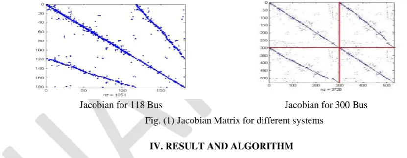
Because the data dependencies are not regular as in Fig.(1), Schur method can be used to separate the unknown variables in interface unknown variables and sub-domain internal unknown variables [18]. That mean, no need for large memory when inverse matrix which will be more powerful in iteration methods by separate their variables. In practice, one needs D to be well-conditioned in order for this algorithm to be numerically accurate.
IV. RESULT AND ALGORITHM
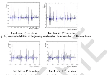
After study and analysis Newton Raphson method to understanding the behaviour of Jacobian Matrix during iterations for different systems (5, 14 and 30 bus), it was noted that values of few elements will slightly changed at beginning of iterations while mostly of them still constants during all iterations. Figures bellow explain this fact:
Jacobian for 118 Bus Jacobian for 300 Bus
Fig. (1) Jacobian Matrix for different systems
Jacobin at 1st iteration Jacobin at 10th iteration
Fig. (2) Jacobin Matrix at beginning and end of iterations for 5 Bus systems
Position in Matrix Position in Matrix
V
a
lu
e
V
a
lu
That mean convergence and divergence will followed the main element values of Jacobian (derivative values) and it is not changed at each iterations. Problems concerning the convergence or divergence tend to be difficult because there are many of roots for each case. Most of ill conditional cases appear to surf ace when system has low R and X line values which effect on solution and it will be fluctuated (Up – Down) near point of root as in fig.(5). These factors will constraining convergence and delivering divergence.
The Schur complement (SC) method can be eliminate or reduce the off-diagonals effects, when it has high values, of Jacobian matrix which make it close to be singular. This matrix will divided to 4 sub-matrices. That mean, it will have separated equations for voltage and voltage angel as follows:
∆𝛿 = 𝑋1(∆𝑃 − 𝑌1∆𝑄) ...(11)
∆𝑉 = 𝑋2(∆𝑄 − 𝑌2∆𝑃)
Where :
𝑋1= 𝐴 − 𝐵𝐷−1𝐶
𝑋2= 𝐷 − 𝐶𝐴−1𝐵
𝑌1= 𝐵𝐷−1
𝑌2= 𝐶𝐴−1
Jacobin at 1st iteration Jacobin at 10th iteration
Fig. (3) Jacobian Matrix at beginning and end of iterations for 14 Bus systems
Jacobin at 1st iteration Jacobin at 10th iteration
Fig. (4) Jacobian Matrix at beginning and end of iterations for 30 Bus systems
5 Bus 14 Bus
Fig.(5). Newton Raphson convergence for 5, 14 and 30 Bus
30 Bus
Position in Matrix Position in Matrix
Position in Matrix Position in Matrix
V
a
lu
e
V
a
lu
e
V
a
lu
e
V
a
lu
e
V
a
lu
e
V
a
lu
e
V
a
lu
e
The off-diagonal matrices like B and C will melt inside inverse of matrix B as term (BD−1C), While second term
(CA−1B ) will has same values of term above if we eliminated rows and columns for (PV Buses) in matrix A which are
already disappeared in Matrix D. It can be considered that X1 equal X2 for same dimensions.
All matrices X1, X2, Y1 and Y2 will slightly changed after each iteration which can considered as constant matrix. In same time, X1 and X2 will tend to be as symmetric matrices and more linearity in their element values. Threshold technique can be used with Y1 and Y2 which has more differences between element values. According to above procedures, the load flow algorithm can be presented as follows:
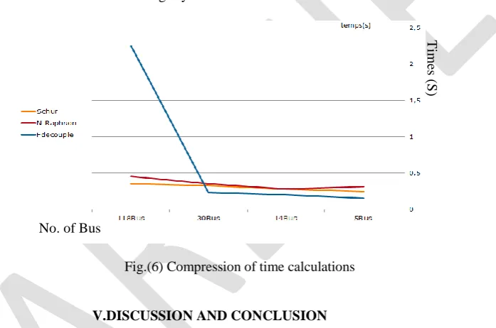
This algorithm has been applied successfully to reduce computation time of load flow iterations, memory required and convergence strategy. Different number of buses has been tested (5, 14,30 and 118) and results has been compared with Newton Raphson (NR) method and Fast Decoupled (FD) method, which shows the efficiency of Schur complement to got good accuracy with less memory and time.
Threshold process has applied successfully to Y1 and Y2 through their values which has high differences to reduce fluctuation in calculations, memory required and computation time. With reference to threshold value which chosen, the value of element should be zero if it below threshold value and no change if it over threshold value. In most of cases, 70% of elements will has zero value if it applied threshold factors for each row. Threshold values for each row can be considered up to 30% of maximum value of elements in the row which will not effect at the accuracy of results. Following table shows results of program for different cases:
Start
Input Network parameters with all initial values required and construct Ybus
Determine Jacobian Matrix as Schur complement for first iteration and calculate ∆𝑉 and ∆𝛿
Accuracy<=0.0001
Update ∆𝑉 and ∆𝛿 then calculate ∆𝑃 and ∆𝑄
Keep matrices of schur as constant and Threshold Y1 and Y2
Calculate new ∆𝑉 and ∆𝛿
Accuracy<=0.0001 Iteration > Max. No
Print Output Results No
Yes
Yes
No. Of Bus 5 14 30 118
SC Accuracy 3.751e-5 0.000106 0.000448 0.000862
Time(s) 0.2496 0.2808 0.3276 0.3588
NR Accuracy 1.01*e-10 0.00072 3.535e-8 4.2797e-5
Time(s) 0.312 0.2808 0.3564 0.4524
FD Accuracy 5.185e-5 0.000749 0.000841 Diverge
Time(s) 0.1560 0.2028 0.2340 2.246
Table (1) Comparison results
The ability of dividing Jacobian matrix by two sub-matrices will allowed to reduce effect of fluctuation up and down near the solution. At same time, it can be observed that performance of algorithm more flexible to find solution with reasonable accuracy and less time. The two separated matrices can be controlled easily, especially when study the stability of system is required. All these features will recommended to use this algorithm to find load flow solution in real applications and in real time calculation for large systems.
Fig.(6) Compression of time calculations
V.DISCUSSION AND CONCLUSION
In this a new algorithm, It has been used schur complement to develop the load flow program, which solve the non linear power flow questions, by separate the Jacobian matrix into two matrices. The first matrix represents the relationship between voltage angles and apparent powers while second matrix represents relationship between voltages and apparent powers. These two matrices are combined to form a direct approach with better convergence, especially when Jacobian matrix is singular. Threshold technique is used to reduce calculations for elements with low values in matrices which has less effective on accuracy of results. This technique is extremely efficient, so that it can be change threshold factor up to 50% which equalized 70% of matrix elements to zero values. This algorithm has been tested different IEEE standard systems and compare it results with Newton Raphson and Fast decoupled methods. Reasonable computation time with less memory and smooth convergence resulted by utilizing this algorithm.
REFERENCES
[1] J.B. Ward and H.W. Ha'le, "Digital Computer Solution of Power Flow Problems", Transactions of the American Institute of Electrical Engineers, vol.75, Issue 3, pp. 398-404, 1956.
[2] J.E. Van Ness, "Iteration Methods for Digital Load Flow Studies", Transactions of the American Institute of Electrical Engineers, vol.78, Issue 3, pp. 583-588, 1959.
[3] W.F. Tinney and C.E. Hart, "Power Flow Solution by Newton's Method", IEEE Transactions on Power Apparatus and Systems, vol. PAS-86, Issue 11, pp. 1449-1456, 1967.
[4] B. Stott and O. Alsac, "Fast Decoupled Load Flow", IEEE Transactions on Power Apparatus and Systems, vol. PAS-93, Issue 3, pp. 859, 1974.
T
im
es (
S)
[5] S. Iwamoto and Y. Tamura, "A Fast Load Flow Method Retaining Nonlinearity", IEEE Transactions on Power Apparatus and Systems, vol. PAS-97, Issue 5, pp. 1586-1599, 1978.
[6] G. X. Luo and A. Semlyen, “Efficient Load Flow for Large Weakly Meshed Networks”, IEEE Transactions on Power Systems, vol. 5, Issue 4, pp. 1309–1316, 1990.
[7] A. Semlyen, “Fundamental Concepts of a Krylov Subspace Power Flow Methodology”, IEEE Transactions on Power Systems, vol. 11, Issue 3, pp. 1528–1537, 1995.
[8] A. J. Flueck and H. D. Chiang, “Solving the Nonlinear Power Flow Equations with an Inexact Newton Method using GMRES”, IEEE Transactions on Power Systems, vol. 13, Issue 2, pp. 267–273, 1998.
[9] Y. Chen and C. Shen, “A Jacobian-free Newton-GMRES(m) Method with Adaptive Preconditioner and Its Application for Power Flow Calculations”, ”, IEEE Transactions on Power Systems, vol. 21, Issue 3, pp. 1096–1103, 2006.
[10] L. M. C. Braz, C. A. Castro, and C. A. F. Murari, “A Critical Evaluation of Step Size Optimization Based Load Flow Methods”, IEEE Transactions on Power Systems, vol. 15, Issue 1, pp. 202–207, 2000.
[11] P. R. Bijwe and S. M. Kelapure, “Nondivergent Fast Power Flow Methods”, IEEE Transactions on Power Systems, vol. 18, Issue 2, pp. 633– 638, 2003.
[12] J. E. Tate and T. J. Overbye, “A Comparison of the Optimal Multiplier in Polar and Rectangular Coordinates”, IEEE Transactions on Power Systems, vol. 20, Issue 4, pp. 1667–1674, 2005.
[13] Rui Bo and Fangxing Li, "Power Flow Studies Using Principal Component Analysis", 40th North American Power Symposium, pp. 1–6, 2008. [14] M. F. Bedriñana and C. A. Castro, "Step Size Optimization Based Interior Point Algorithm: Applications and Treatment of Ill conditioning in
Optimal Power Flow Solutions", IEEE Power and Energy Society General Meeting, pp. 1-8, 2009.
[15] F. Milano,"Continuous Newton’s Method for Power Flow Analysis", IEEE Transactions on Power Systems, Vol. 24, Issue 1, pp. 50-57, 2009. [16] Hadi Saadat, "Power System Analysis", McGraw-Hill, 1999.
[17] P. Aristidou, D. Fabozzi, and T. V. Cutsem, "Dynamic Simulation of Large-scale Power Systems Using a Parallel Schur-complement-based Decomposition Method", IEEE Transactions on Parallel and Distributed Systems, Vol. PP, Issue 99, 2013 .
[18] D. Guibert, D. Tromeur-Dervout, "A Schur Complement Method for DAE/ODE Systems in Multi-Domain Mechanical Design", Lecture Notes in Computational Science and Engineering, Vol. 60, pp. 535–541, 2008.
APPENDIX A
Parts of the Jacobian matrix can be calculated with following equations:
𝜕𝑃𝑘
𝜕𝛿𝑘 (𝑥)
= 𝑉𝑘 𝑉𝑗 |𝑌𝑘𝑗|sin(Ɵ𝑘𝑗− 𝛿𝑘+ 𝛿𝑗) 𝑗 ≠𝑘
J1 diagonal element
𝜕𝑃𝑘
𝜕𝛿𝑗 (𝑥)
= − 𝑉𝑘 𝑉𝑗 |𝑌𝑘𝑗|sin(Ɵ𝑘𝑗− 𝛿𝑘+ 𝛿𝑗)
J1 off diagonal element
𝜕𝑃𝑘
𝜕|𝑉𝑘| (𝑥)
= 2 𝑉𝑘 |𝑌𝑘𝑘|𝑐𝑜𝑠𝜃𝑘𝑘+ 𝑉𝑗 |𝑌𝑘𝑗|cos(Ɵ𝑘𝑗− 𝛿𝑘+ 𝛿𝑗) 𝑗 ≠𝑘
J2 diagonal element
𝜕𝑃𝑘
𝜕|𝑉𝑗| (𝑥)
= 𝑉𝑘 |𝑌𝑘𝑗|cos(Ɵ𝑘𝑗− 𝛿𝑘+ 𝛿𝑗)
J2 off diagonal element
𝜕𝑄𝑘
𝜕𝛿𝑘 (𝑥)
= 𝑉𝑘 𝑉𝑗 |𝑌𝑘𝑗|cos(Ɵ𝑘𝑗− 𝛿𝑘+ 𝛿𝑗) 𝑗 ≠𝑘
J3 diagonal element
𝜕𝑄𝑘
𝜕𝛿𝑗 (𝑥)
= − 𝑉𝑘 𝑉𝑗 |𝑌𝑘𝑗|cos(Ɵ𝑘𝑗− 𝛿𝑘+ 𝛿𝑗)
J3 off diagonal element
𝜕𝑄𝑘
𝜕|𝑉𝑘| (𝑥)
= −2 𝑉𝑘 𝑌𝑘𝑘 𝑠𝑖𝑛𝜃𝑘𝑘− 𝑉𝑗 |𝑌𝑘𝑗|sin(Ɵ𝑘𝑗− 𝛿𝑘+ 𝛿𝑗) 𝑗 ≠𝑘
J4 diagonal element
𝜕𝑄𝑘
𝜕|𝑉𝑗| (𝑥)
J4 off diagonal element
The general form of the method will be:
△ 𝑃2
⋮ △ 𝑃𝑛−1
△ 𝑄2
⋮ △ 𝑄𝑛−𝑛𝑔 −1
𝜕𝑃2
𝜕𝛿2
⋱ 𝜕𝑃𝑛−1
𝜕𝛿𝑛−1
𝜕𝑃2
𝜕|𝑉2|
⋱
𝜕𝑃𝑛−1
𝜕|𝑉𝑛−𝑛𝑔 −1|
𝜕𝑄2
𝜕𝛿2
⋱
𝜕𝑄𝑛−𝑛𝑔 −1
𝜕𝛿𝑛−1
𝜕𝑃𝑘
𝜕|𝑉𝑘|
⋱ 𝜕𝑃𝑘
𝜕|𝑉𝑘|
△ 𝛿2
⋮ △ 𝛿𝑛−1
△ |𝑉2|
⋮ △ |𝑉𝑛−𝑛𝑔 −1|
N bus general form of N-R method with