62:3 (2013) 15–20 | www.jurnalteknologi.utm.my | eISSN 2180–3722 | ISSN 0127–9696
Full paper
Jurnal
Teknologi
Evaluation of Different EEG Source Localization Methods Using Testing
Localization Errors
Leila SaeidiAsla*, Tahir Ahmada
aDepartment of Mathematical Sciences, Faculty of Science, Universiti Teknologi Malaysia, 81310 UTM Johor Bahru, Johor, Malaysia
*Corresponding author: [email protected]
Article history
Received :18 March 2013 Received in revised form : 26 April 2013
Accepted :17 May 2013
Graphical abstract
Abstract
The ideas underlying the quantitative localization of the sources of the EEG review within the brain along with the current and emerging approaches to the problem. The ideas mentioned consist of distributed and dipolar source models and head models ranging from the spherical to the more realistic based on the boundary and finite elements. The forward and inverse problems in electroencephalography will debate. The inverse problem has non-uniqueness property in nature. More precisely, different combinations of sources can produce similar potential fields occur on the head. In contrast, the forward problem does have a unique solution. The forward problem calculates the potential field at the scalp from known source locations, source strengths and conductivity in the head, and it can be used to solve the inverse problem. In the final part of this paper, we compare the performance of three well-known EEG source localization techniques which applied to the underdetermined (distributed) source localization of the inverse problem. These techniques consist of LORETA, WMN and MN, which comparing by testing localization error.
Keywords: Inverse /forward problem; comparative test of tomographic techniques; LORETA, WMN and MN
Abstrak
idea yang mendasari penyetempatan kuantitatif sumber kajian EEG dalam otak bersama-sama dengan pendekatan semasa dan baru muncul untuk masalah. Idea-idea yang disebut terdiri daripada model sumber teragih dan dipolar dan model kepala terdiri daripada sfera untuk lebih realistik berdasarkan sempadan dan unsur terhingga. Masalah hadapan dan songsang di electroencephalography akan berdebat. Masalah songsang bukan keunikan harta dalam alam semula jadi. Lebih tepat, kombinasi sumber yang berlainan boleh menghasilkan bidang berpotensi yang serupa berlaku di kepala. Sebaliknya, masalah hadapan tidak mempunyai penyelesaian yang unik. Masalah hadapan mengira bidang yang berpotensi pada kulit kepala dari lokasi sumber diketahui, kekuatan sumber dan kekonduksian di kepala, dan ia boleh digunakan untuk menyelesaikan masalah songsang. Dalam bahagian akhir kertas ini, kita bandingkan prestasi tiga terkenal EEG teknik penyetempatan sumber yang memohon kepada underdetermined (diedarkan) sumber penyetempatan masalah songsang. Teknik-teknik ini terdiri daripada Loreta, WMN dan MN, yang membandingkan dengan kesilapan penyetempatan ujian.
Kata kunci: Masalah songsang/Forward; ujian perbandingan tomografi teknik; Loreta; WMN dan MN
© 2013 Penerbit UTM Press. All rights reserved.
1.0 INTRODUCTION
EEG Source Localization techniques intends to localizing active sources inside the brain from measurements of the electromagnetic field they produce, which can be measured outside the head. This localization problem is commonly referred to as the inverse source problem of electroencephalography. They are ill-posed in general, mostly due to the lack of continuity and stability, but also to non-uniqueness.1 By introducing reasonable a priori restrictions, the inverse problem can be solved and the most probable sources in the brain can be accurately localized. 4
Electroencephalography (EEG) is non-invasive measuring approach to evaluate and characterize neural electrical sources in a human brain.2,3 EEG measure electric potential differences and extremely weak magnetic fields produced by the electric activity of the neural cells, correspondingly.
imaging should involve many more analysis steps than applying a given source localization algorithm to the data.
Different signal processing techniques used to derive the hidden information from the signal. In order to determine the area of an electrical source in the brain using the signal processing techniques, it is essential to postulate a model of the source and a model of the head.
In general, model of the source can be classified into two main categories: dipolar model and distributed source model. In dipolar model, the electric sources are equal to one or few. It will lie close to the center of the actual generator area, have an orientation that is orthogonal to the net orientation of this cortex, but locate slightly deeply to the cortex. 11In calculated n several studies; we noted that dipole orientation gave an essential signal to distinguishing foci in different temporal lobe regions, 12 and also, researcher found that dipole orientation, instead of strictly dipole location, more clearly differentiates among possible cortical foci. For this reason, most seizures are modeled by equivalent dipoles13.
Distributed source model considers the dipoles are distributed often in cerebral volume according to a 3D grid. The dipole’s positions are fixed, and their amplitudes should be estimated. Head model is another assumption to compute the inverse solution for the location of the source in the model. Head models ranging from the spherical to the more realistic based on the boundary and finite elements. The spherical head model contains concentric layers with different electrical conductivities, which represent the skull, scalp, etc.More realistic head models can be created using finite elements or boundary elements. These head models can be adjusted to extremely closely approximate a real head. Realistic head shapes, rather than the spherical head model, has been shown to cause dipole and other forms of EEG source modeling more accurate by up to 3 cm in focus localization.14
The first contribution of this paper includes a short review of the concepts of instantaneous, 3D, discrete, linear solutions for the Forward/inverse problems of EEG. Afterwards, the final results presented here correspond to a comparison of three different tomographies taken from the literature.
2.0 METHODS
Nowadays, rising computational power has given researchers the tools to go a step further and try to locate the hidden sources which promote the tools (EEG). This activity is call EEG source localization .15Several methods have proposed for EEG source localization. These methods were formulated based on the inverse problem and forward problem. Forward problem computes the electrode potentials at the scalp given the source distribution in the brain. Inverse problem calculates the source distribution out of the measured scalp EEG based on the forward solution.
2.1 EEG Forward Calculation’s Method
The sources of brain activity cause electrical fields according to Maxwell's and Ohm's law. Because of the high propagation velocity of the electromagnetic waves, the currents caused by the sources in the brain behave in a stationary way. This means that no charge is accumulated at any time in the brain. Therefore, it can be stated that for any current density J: 16
.J 0 (2.1)
In the case, of a stationary current, the electric field E is related to the electric potential V by the following expression:
E
V
(2.2) The minus sign indicates that the electric field is orientated from an area with a high potential to an area with a low potential.17The current density in the head related with neural activation is the sum of the primary current, related to the original neural activity and a passive current flowσE:JJpE (2.3)
where, is the conductivity of the head tissues. The primary currents are of interest when solving the inverse problems because they represent neuronal activation. However, the consequences of volume currents must still be regarded when solving the forward problem since they contribute to the scalp potentials.18Taking the divergence of both sides of equation 2.3 gives:
.Jp .E (2-4) Substituting equation 2.2 in equation 2.4 gives the Poisson equation for the potential field:
.Jp .( V) (2-5) When the medium is assumed to be infinite, isotropic and homogeneous, it can be proven that the solution of the Poisson equation is:16
0
0
.
1
( )
4
p volume
J
V r
r
r
(2-6)which gives the value of the potential at a point r0, in the volume conductor resulting from a current density Jp.
Unfortunately, the human head is not isotropic and homogeneous, and it has an irregular shape. To solve the Poisson equation for realistic head shapes, numerical solution methods are needed.
- Finite element method (FEM) - Boundary element method (BEM) -Finite difference method (FDM)
Regarding to application, one should appropriate method selected, and additional assumptions need to be made. For instance, when FEM and BEM are used to solve the Poisson equation, the head is divided into three sublayer: the brain, the skull and the scalp, with each a different conductivity. These conductivities are usually standard values that have been measured in vitro using postmortem tissue19.
These numerical solution models allow incorporating the realistic geometry of the head and brain after reconstruction of the anatomical structure from individual data sets. Previous studies20 have found that a more realistic head model performs better than a less complex, for example, spherical, head model in EEG simulations, because volume currents are more accurately taken into account. In particular, the BEM approach is able to improve the source reconstruction in comparison with spherical models. Mostly in basal brain areas, including the temporal lobe 21because it gathers a more realistic shape of brain compartments of isotropic and homogeneous conductivities by using closed triangle meshes.22The FDM and the FEM provide better accuracy than the BEM because they provide a better representation of the cortical structures, such as sulci and gyri in the brain, in a three-dimensional head model. 23
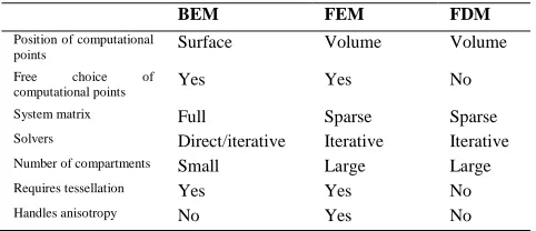
FDM, the solution of the forward problem is calculated in the entire volume.24Following table, explain all differences between BEM, FEM and FDM base on realistic head model.4
Table 1 A comparison of the three methods for solving equation of Poisson in a realistic head model (Wendel et al., 2009)
BEM FEM FDM
Position of computational
points Surface Volume Volume Free choice of
computational points Yes Yes No System matrix Full Sparse Sparse
Solvers Direct/iterative Iterative Iterative
Number of compartments Small Large Large
Requires tessellation Yes Yes No
Handles anisotropy No Yes No
2.2 EEG Inverse Estimation’s Method
Nowadays, various methods have been developed to solve the inverse problem for EEG source localization and these methods can be solved using variety methods based on the assumptions made. The main purpose of EEG inverse problem is to evaluate neural current sources from exterior electromagnetic measurements. These types of inverse problems have suffered from a variety of obstacles for instance, high sensitivity to noise, ill-posed characteristic, and difficulty in verification and so on. Various approaches and algorithms have been studied; to solve problems and evaluate the brain sources more efficiently.5 Three types of source models are commonly used:
- Equivalent current dipoles (ECD) method - Distributed source localization method - Scanning methods
The ECD model assumes small numbers of current dipoles to approximate the flow of electrical current in a small brain region. It has been shown to be a great exploration tool in several cognitive and clinical applications.12,25 The main advantages of the ECD model are that it is extremely simple to implement and is robust to noise. To implement the ECD model, however, the numbers of ECDs should be determined a priori, which is often extremely challenging due to lack of initial information. Additionally, final solutions are highly dependent on initial assumptions for the ECDs.26
Another disadvantage of the ECD model is that it has a large possibility of being fitted outside the grey matter of the cerebral cortex, since conventional ECD models have not regarded any anatomical information on the brain.
On the contrary to the ECD model, the distributed source model assumes a lot of current dipoles scattered in limited source spaces, orientations and/or strengths of the dipoles are then verified using linear or nonlinear estimation methods.6,27,28,29 The distributed source application does not require initial information on the numbers and preliminary locations of brain activations, which allows inexperienced users to localize EEG sources more easily. Furthermore, the distributed source model is physiologically more reasonable than the ECD model, because it restricts the feasible source space based on the real brain anatomy. When the distributed source model is applied to focal source localizations, we usually regard local peak positions of the source distributions as the locations of the brain sources .15, 30
The third approach to overcome the problem of local minima is the use of a scanning method. These methods use a discrete grid to search for optimal dipole positions throughout the source volume. Source locations are then determined as those for which a metric computed at that location exceeds a given threshold. While these approaches do not lead to a true least squares solution, they can be used to initialize a local least squares search .18
2.3 Simulated Measurements
In this section, we discuss some related issues related to the measurement of the source imaging. We start with the following theory: 4
2.3.1 Theory
The relationship between the sources J inside the head and the
outside measurements
is described as
KJ
(Eq.1)ϕ is an N×1-matrix comprised of measurements of scalp electric potential differences. The coordinates of the measurement points are given by the Cartesian position vectors. The 3M×1-matrix
1,
2,...,
TT T T
M
J
j
j
j
is comprised of the current densities,
at M points within the brain volume, with
=1, …, M. The super-script “T” indicates transpose. The coordinates of the source points inside the brain volume are known by the Cartesianposition vector. The N×3M-matrix K is a transfer matrix. The
th row of the matrix K, with
=1, …, N is
1,
2,...,
T T T
M
K
K
K
where
,
,
T
T T T
x y z
K
K
K
K
is the lead field.Generally, the EEG inverse solution can be written as: 31
J
T
(Eq.2) where the 3M×N matrix T is some generalized inverse of the transfer matrix K which must satisfy,
KT
H
N (Eq.3) whereH
N indicates the N×N average reference operator.Eq. (3) states the fact that the estimated current density (i.e., the inverse solution) given by Eq. (2) must satisfy the measurements in forward equation (Eq.1) The majority of the well-known solutions (linear and nonlinear) of the EEG inverse problems are ill-posed. i.e. it is identified to have infinite solutions. More precisely, there exist an infinite number of different generalized inverse matrices T, all producing current densities J (Eq. 2) that satisfy the original measurements ϕ (Eq. 1).
2.4 The Resolution Matrix
The main problem now is: what criterion should be used for selecting an inverse solution? The quality of any given instantaneous, 3D, discrete, linear inverse solution for EEG can be analyzed in terms of the resolution matrix of Backus and Gilbert (Backus, 1968) Substituting Eq. (1) in (2) gives the following relation between “true (J)” and “estimated (J)” current densities:
J
est.
R J
tr. (Eq.4)where R is resolution matrix .31
Now, we discuss the properties of a given inverse solution, founded on its resolution matrix: by means of the collection of all columns. A column of the resolution matrix corresponds to the “estimated” current density for a “true” point source. This can be seen directly from Eqs. (4) and (5), when the true, current density, contains zeros everywhere, except for unity at some given element. The estimated current density in this condition is known as the “point spread function.”
The aim of any tomography is the property of correct localization. As a result, the only relevant way of testing a linear tomography is to analyze the estimated images produced by ideal point sources. Such tomographic images are exactly the point spread functions. If these images have incorrectly located peaks, then the process does not justify the name of “tomography”, because of the lack of any localization capability.33
2.5 Specific Inverse Solution
2.5.1 Problem Statement
For any given definite matrix W of dimension 3M⨯3M, solve the following problem,
min
T,
int:
J
J WJ under constra
KJ
The Minimum Norm Solution:
The inverse solution base on Minimum Norm (MN) estimation as following,
1 1
, : T[ T]
J T with T W K KW K
where
1
[
T]
KW K
indicates the Moore-Penrose Pseudo inverseof
1
[
T]
KW K
. This solution based on Hamalainen andllmoniemi studies with W=I(3M). 34 In next approach about the inverse solution corresponds to the generalized inverse matrix T that optimizes, in a weighted sense, the resolution matrix.
Problem statement: find the minimization of deviation of the resolution matrix from ideal behavior as following problem:
1
min [( ) ( ) ]
(3 ) (3 )
T
tr I TK W I TK
T M M
where I(3M) is the 3M×3M identity matrix, and “tr” denotes the trace of a matrix.
2.5.2 The Weight Minimum Norm Solution:
According to Marqui,31 has proven that the weighted minimum norm (WMN) solution corresponds to
3
W I ,
where
indicates the Kronecker product, I3 is the identity 3×3-matrix, and
is a diagonal M×M-matrix with,1
,
1,...,
N T
K K
for
M
.
2.5.3 The Low Resolution Brain Electromagnetic Tomography (LORETA)
LORETA combines the lead-field normalization with the Laplacian operator, therefore, gives the depth-compensated inverse solution under the limit of smoothly distributed sources. It is based on the maximum smoothness of the solution. It normalizes the columns of G (gain matrix) to give all sources (close to the surface and deeper ones) the same opportunity of being reconstructed.
In LORETA, sources are distributed in the entire inner head volume. In this situation, L (D) = ||ΔB.D||2 , and B = Ω ^ I3 is a diagonal matrix for the column normalization of G. 35
1
( T T ) T
DLOR G G B B G M
or
1
1 1
( T ) T( ( T ) T )
DLOR B B G G B B G I M
N
3.0 COMPARATIVE TEST OF TOMOGRAPHIC TECHNIQUES
The aim of a tomography is localization. Hence, as a first comparative test of tomographic techniques for EEG, the main feature of interest is the localization error.
Pascual-Marqui3 has shown that all the information on localization error of a tomography is given by the set of all columns of the resolution matrix (Eq. (5)).
Regarding to Eq. (4), consider an ideal “true” point source
defined as
J
tr.
Y
, where Ya is the
th column of the3M⨯3M identity matrix. The position in 3D space for the
thvoxel(point) is 1
vc
, where “c” (taking values in the range 1…M) is given by:1
( 1) 1 int
3
C
(Eq.6)
Where “int[r]” indicates the “integer part of r”. From Eqs. (4) and (5), the corresponding 3D tomographic representation is given by:
.
( , , ,...,
1 2 3 3)
Test M
J
TKY
j j j
j
(Eq.7) which is the
th column of the resolution matrix (or point spread function). The least of all characteristics that a tomography must possess is that images of the point spread functions have their maxima located as accurately as possible. This characteristic is an essential requirement for accurate localization. The locationof the point spread function maximum is 2
vc
where:
2
( 1) 1 int
3
C
(Eq.8)
and:
arg
Max
j
(Eq.9)L vc1vc2 (Eq.10)
For all point, spread functions .31
4.0 RESULTS AND DISCUSSION
To achieve to comparison between different source localization methods, in the brain in 3D, we used information which is collected from EEG recordings during epilepsy provided by the Hospital Kuala Lumpur, Malaysia.
The major requirements for making a reasonable and fair comparison are to use the same measurement space, the same solution space, and the same head model .36 The model of head is assumed to be the union of three disjoint homogeneous spherical layers with unit radius. The measurement space includes 148 electrodes covering the scalp surface. They are demonstrated in Figure 3.
The solution space consists of 818 grid points (voxels) corresponding to a 3D regular cubic grid with minimal inter-point distance d=0.133, confined to a maximum radius of 0.8, with vertical coordinate values
Z
0.4
.In EEG data, average reference measurement were used, with electrodes having the same coordinates as the magnetic sensors, but scaled to a radius of 1.The sensor coordinates used here were proposed by Lutkenhoner and Mosher37 and are illustrated in Figure 3.
Figure 3 3D illustration of the measurement space defined by 148 scalp EEG electrodes. A unit radius, three-concentric spheres model is used for the head. (Marqui, 1999)
Figure 5 Demonstration of the measurement space explaind by scalp EEG electrodes((Marqui, 1999)
Localization errors got from the resolution operators of the different inverse solutions, are summarized in Table 1 in terms of their frequency distributions the algorithm based on Marqui.31The results reveal the superiority of LORETA over minimum norm and over weighted minimum norm. Also, we extract all localization errors of tomographies. In each row, the number of horizontal tomographic slices through the brain corresponds to a variety inverse method. Localization errors are gray-color coded in the slices, with white representing zero localization error, and black indicating 7 or more grid units of localization error.
Table 1 Localization errors are summarized as percent of test source(dipole) that were localized with errors in the rang indicated in the first column (1 unit=minimmum grid inter-point distance)
Localization
Error LoRETA LoRETA MN MN WMN WMN
% Cum. % % Cum.
% % Cum.% (0.0,0.5) 17.52 17.52 11.42 11.24 11.24 11.24 (0.5,1.0) 0 17.52 0 11.24 0 11.24 (1.0,1,5) 78.32 95.84 39.78 51.02 36.9 48.14 (1.5,2.0) 0.65 96.49 6.71 57.73 13.73 61.87 (2.0,2.5) 3.47 96.96 18.79 76.52 17.65 79.52 (2.5,3.0) 0 96.96 1.06 77.58 2.06 81.58 (3.0,3.5) 0.04 100 10.32 87.9 10.87 92.45 (3.5,4.0) 0 100 2.8 90.7 3.12 95.57 (4.0,4.5) 0 100 6.34 97.04 3.92 99.49 (4.5,5.0) 0 100 0.9 97.94 0.29 99.78 (5.0,5.5) 0 100 2.06 100 0.22 100
5.0 CONCLUSION
This result demonstrates that LORETA has a reasonable, low localization error of 1 grid unit in the average. We have afforded to write an article that benefits the novice, and focuses much needed assistance to numerous open issues like epileptogenic foci.
Acknowledgement
The authors would like to thank the Malaysian Ministry of Higher Education and Universiti Teknologi Malaysia for International doctoral Fellowship(IDF).
References
[1] Baratchart, L.,Ben Abda, A, Ben Hassen, F. and Leblond, J. 2005. Recovery of Pointwise Sources rr Small Inclusions in 2D Domains and Rational Approximation. Inverse Problems. 21: 51–74.
[2] Hämäläinen, M. S., R. Hari, R. J. Ilmoniemi, J. Knuutila, and O. V. Lounasmaa. 1993. Magnetoencephalography. Theory, Instrumentation and Applications to the Noninvasive Study of Human Brain Function.
Rev. Mod. Phys. 65: 413–497.
[3] Malmivuo. J. and R. Plonsey. 1995. Bioelectromagnetism. Oxford Univ. Press.
[4] Wendel, K., Väisänen, O., Malmivuo, J., Gencer, N. G, Vanrumste, B., Durka, P. J., Magjarevic, R., Selma Supek, S., Pascu, M. P., Fontenelle, H., Menendez, R. G. D. P. 2009. EEG/MEG Source Imaging: Methods, Challenges, and Open Issues. Computational Intelligence and Neuroscience. Article ID 656092, 12.
[6] Fuchs. M., Wagner, M., Kohler, T. and Wischmann, H-A. 1999. Linear and Nonlinear Current Density Reconstructions. J. Clin. Neurophysiol.
16: 267–95.
[7] George, J. S., Aine, C. J., Mosher, .J. C., Schmidt, D. M., Ranken, D. M., Schlitt, H. A., Wood, C. C., Lewine, .J. D., Sanders, .J. A., Belliveau. J. W. 1995. Mapping Function in the Human Brain with Magnetoencephalography, Anatomical Magnetic Resonance Imaging, And Functional Magnetic Resonance Imaging (Review). J Clin Neurophysiol. 12: 406–31.
[8] Gonzalez Andino, S., van Dijk, B. W., De Munck, J. C., Grave de Peralta, R., Kno¨sche, T. 1999. Source Modeling. In: Uhl C, editor. Analysis of Neurophysiological Brain Functioning. Berlin: Springer. 148–228.
[9] Grave de Peralta Menendez, R., Gonzalez Andino, S. L. 1998. A Critical Analysis of Linear Inverse Solutions. IEEE Trans Biomed Eng.
45: 440–8.
[10] He. B., Lian, J. 2002. High-resolution Spatio-temporal Functional Neuroimaging of Brain Activity (Review). Crit Rev Biomed Eng. 30: 283–306.
[11] Pascual-Marqui, R. D. 1999.Review of Methods for Solving the EEG Inverse problem. IJBEM. 1(1): 75–86 .
[12] Ebersole, J. S. 1994. Noninvasive Localization of the Epileptogenic Focus by EEG Dipole Modelling. Acta Neurol. Scand. 152(l): 20–28. [13] Ebersole, J. S. Functional Neuroimaging with Eeg Source Models to
Localize Epilep-togenic Foci Noninvasively. University of Chicago Hospitals' Clinical Comment.
[14] Ebersole, J. S., Hawes, S. M. 1997. Spike/seizure Dipoles Derived from Realistic Head Models Accurately Portray Temporal Lobe Foci.
Epilepsia. 38(8): 66.
[15] Baillet, S., Riera, J. J., Marin, G., Mangin, J. F., Aubert, J. and Garnero, L. 2001b. Evaluation of Inverse Methods and Head Models for EEG Source Localization Using a Human Skull Phantom. Phys. Med. Biol. 46: 77–96.
[16] Jackson, J. 1984. Classical Electrodynamics. Academic Press Inc. Third ed.
[17] Hallez, H, Vanrumste, B., Grech, R., Muscat, J., Clercq, W. D., Vergult, A., D'Asseler, Y., Camilleri, K. P., abri, S. G., Huffel, S. V. and Lemahieu, I. 2007. Review on Solving the Forward Problem In EEG Source Analysis. Journal of NeuroEngineering and Rehabilitation. 4: 46.
[18] Darvas, F., D. Pantazis, E. Kucukaltun-Yildirim, and R. M. Leahy. 2004.Mapping Human Brain Function with MEG and EEG: Methods and Validation. NeuroImage. 23: S289–S299.
[19] Geddes, L. A. and Baker, L. E. 1967. The Specific Resistance of Biological Material–A Compendium of Data for the Biomedical Engineer and Physiologist. Med. Biol. Eng. 5: 271.
[20] Vatta. F., P. Bruno, and P. Inchingolo. 2005. Multiregion bicentric-Spheres Models of the Head for the Simulation of Bioelectric Phenomena. IEEE Transactions on Biomedical Engineering. 52(3):384– 389.
[21] Fuchs, .M., M. Wagner, and J. Kastner. 2001. Boundary Element Method Volume Conductor Models for EEG Source Reconstruction.
Clinical Neurophysiology. 112(8): 1400–1407.
[22] Fuchs, M., M. Wagner, and J. Kastner. 2007. Development of Volume Conductor and Source Models to Localize Epileptic Foci. Journal of Clinical Neurophysiology. 24(2): 101–119
[23] Ramon, C., J. Haueisen, and P. H. Schimpf. 2006.Influence of head models on neuromagnetic fields and inverse source localizations.
BioMedical Engineering Online. 5: 55.
[24] Barnard, A. C. L., Duck, I. M., and M. S. Lynn. 1967. The Application of Electromagnetic Theory to Electrocardiography—I: Derivation Of the Integral Equations. Biophysics Journal. 7: 443–462.
[25] De Munck, J. C., van Dijk, B. W., and Spekreijse, H. 1988. Mathematical Dipoles are Adequate to Describe Realistic Generators of Human Brain Activity. IEEE Trans. Biomed. Eng. 35: 960–966. [26] Uutela, K., H¨am¨al¨ainen. M and Salmelin, R. 1998. Global
Optimization in the Localization of Neuromagnetic Sources. IEEE
Trans. Biomed. Eng. 45: 716–23.
[27] Dale, A. M. and Sereno, .M. I.1993. Improved Localization of Cortical Activity by Combining EEG and MEG with MRI Surface Reconstruction. A Linear Approach J. Cognit. Neurosci. 5: 162–76. [28] Im, C-H., An, K-O., Jung, H-K., Kwon, H. and Lee, Y-H. 2003.
Assessment Criteria forMEG/EEG Cortical Patch. Tests Phys. Med. Biol. 48: 2561–73.
[29] Bonmassar, G., Schwartz, D. P., Liu, A. K., Kwong, K. K., Dale, A., Mand Belliveau, J. W. 2001. Spatiotemporal Brain Imaging of Visual-Evoked Activity Using Interleaved EEG and fMRI Recordings.
Neuroimage. 13(10): 35–43.
[30] Jerbi. K., Mosher, .J .C., Nolte, G., Baillet, S., Garnero, L. and Leahy, R. M. 2002. From Dipoles to Multipoles: Parametric Solutions to the Inverse Problem in MEG Proc. Conf. on Biomagnetism—BIOMAG. [31] Pascual-Marqui, R. D., Lehmann, D., Koenig, T., Kochi, K., Merlo M.
C. G., Hell, D., Koukkou, M. 1999. Low Resolution Brain Electromagnetic Tomography (LORETA) Functional Imaging in Acute, Neurolepticnaive, First-Episode, Productive Schizophrenics. Psychiatry Research: Neuroimaging.
[32] Backus, G., and Gilbert, F.1968. The Resolving Power of Gross Earth Data. Geophys. J. R. Astr. Soc.16: 169–205.
[33] Golub, G. H. and Van Loan, C. F. 1983. Matrix Computation. Baltimore, MD: The John Hopkins University. Press.
[34] Hämäläinen, M. S. and Ilmoniemi, R. J. 1984. Interpreting Measured Magnetic Fields of the Brain: Estimates of Current Distributions. Technical Report TKK-F-A559, Helsinki University of Technology. [35] Koles, Z. J. 1998.Trends in EEG source localization. Electroenceph.
clin. Neurophysiol. 106: 127–137.
[36] Ary, J. P., Klevin, S. A., and Fender, D. H. 1981. Location of Sources of Evoked Scalp Potentials: Corrections for Skull and Scalp Thickness.
IEEE Trans. Biomed. Eng. 28: 447–452.