8-19-2015 12:00 AM A Study Of Green’s Relations On Algebraic Semigroups

(1)

Western University Western University

Scholarship@Western

Electronic Thesis and Dissertation Repository

8-19-2015 12:00 AM

A Study Of Green’s Relations On Algebraic Semigroups

Allen O'Hara

The University of Western Ontario

Supervisor Lex Renner

The University of Western Ontario Graduate Program in Mathematics

A thesis submitted in partial fulfillment of the requirements for the degree in Doctor of Philosophy

Follow this and additional works at: https://ir.lib.uwo.ca/etd

Part of the Algebraic Geometry Commons

Recommended Citation Recommended Citation

O'Hara, Allen, "A Study Of Green’s Relations On Algebraic Semigroups" (2015). Electronic Thesis and Dissertation Repository. 3047.

https://ir.lib.uwo.ca/etd/3047

This Dissertation/Thesis is brought to you for free and open access by Scholarship@Western. It has been accepted for inclusion in Electronic Thesis and Dissertation Repository by an authorized administrator of

(2)

(Thesis format: Monograph)

by

Allen O’Hara

Graduate Program in Mathematics

A thesis submitted in partial fulfillment

of the requirements for the degree of

Doctor of Philosophy

The School of Graduate and Postdoctoral Studies

The University of Western Ontario

London, Ontario, Canada

c

(3)

Acknowledgements

First and foremost, I would like to thank my supervisor, Lex Renner, who was phenomenal

in his support and encouragement. Having been one of the first in the field of linear algebraic

monoids, I had much to learn from him and he made it not a task but a pleasure. Our meetings

have been fantastic and he was always eager to share his wisdom and enthusiasm.

Many thanks go to my colleagues, not just those from Western but all those I have worked

with in my academic career. Each of them helped shape the mathematician I am today and will

be in the future.

I would like to thank my friends and family for their love and support. Special mention

goes to my parents, who taught me to dream and to never stop until I exceeded my potential.

Lastly, I wish to acknowledge my darling wife, Elise. She is the light of my life, and when

I am with her I feel like I can accomplish anything. I would like to dedicate this work to her.

It has been a hell of a ride. I cannot wait to see where I go next!

(4)

The purpose of this work is to enhance the understanding regular algebraic semigroups

by considering the structural influence of Green’s relations. There will be three chief topics of

discussion.

◦Green’s relations and the Adherence order on reductive monoids ◦Renner’s conjecture on regular irreducible semigroups with zero

◦a Green’s relation inspired construction of regular algebraic semigroups

Primarily, we will explore the combinatorial and geometric nature of reductive monoids

with zero. Such monoids have a decomposition in terms of a Borel subgroup, called the Bruhat

decomposition, which produces a finite monoid,R, the Renner monoid. We will explore the structure ofRby way of Green’s relations. In particular, we will be exploring the nature of the Adherence order poset, (R,≤) when restricted toJ-,R-,L-, andH -classes.

From reductive monoids we broaden the impact of Green’s relations and explore regular

algebraic semigroups. Specifically, we resolve Renner’s conjecture and show that the supports,

X` = J/R and Xr = J/L are projective varieties. Spurred on by the result, we use

in-variant theory to generalise the Rees matrix construction for algebraic semigroups to construct

irreducible regular semigroups with 0. Our construction will start with specified maximal

classes,Re,Le, andHeand reconstruct an entire semigroup. In a lengthy example, we will use

some of our previous combinatorial results to apply the construction to a natural generalisation

of determinantal varieties.

Highlights include the unique “vanilla form” decomposition for elements of the Renner

monoid (Definition 5.36), a proof of Renner’s conjecture on the projectiveness of supports for

irreducible regular semigroups with zero (Theorem 8.40), and the construction of irreducible

regular semigroups from prespecified maximalR- andL-classes (Definition 9.6).

Keywords: Algebraic semigroups, reductive monoids, Green’s relations, Adherence order,

Renner monoid, semigroup supports, irreducible regular algebraic semigroups with zero

(5)

List of Appendices

Results From Other Sources . . . 151

Opposite Standard Form . . . 152

Pointed ParabolicJ-classes onM3(K) . . . 155

(9)

1

1 Introduction

The systematic investigation of linear algebraic semigroups and reductive algebraic monoids

was pioneered around 1980 by Mohan Putcha and my supervisor, Lex Renner. Since then, the

discipline has blossomed into a coherent branch of algebra involving embedding theory,

repre-sentation theory and algebraic combinatorics. One of the most important features of a reductive

monoid is the existence of the Bruhat Decomposition. More precisely, the Bruhat

decomposi-tion, which is much studied for groups, extends to a perfect analogue for reductive monoids.

This monoid Bruhat decomposition allows us to express the monoid as a disjoint union

of double cosets (for a given Borel subgroup) indexed by a finite structure called the Renner

monoid (the monoid analogue of the Weyl group). The importance of this decomposition is

that it allows many questions about the nature and structure of the monoid to become simpler

questions about the Renner monoid.

Unlike groups, semigroups and monoids bring an additional structure in the form of Greens

relations, which characterise the elements of the semigroup in terms of the ideals they generate.

So important are Greens relations that Scottish semigroup theorist, John Mackintosh Howie,

once said, “on encountering a new semigroup, almost the first question one asks is ‘What are

the Green relations like?’ ”. In reductive monoids, we denote these relations by J, L, R

andH. A natural question is how do these relations interact with the Bruhat decomposition?

What additional information can they tell us?

Of particular focus is the H relation, which has many interesting and desirable

proper-ties. H -classes most closely resemble groups (indeed theH -class of an idempotent element

forms a group), and so their structure is the one most likely to form a bridge between the

Ren-ner monoid and the information we know from the better understood Weyl groups. One way

we can investigate this structure is by decomposing our monoid, not in terms of the Bruhat

decomposition, which is indexed by elements of the Renner monoid, but in terms of a disjoint

union of double cosets of the H -classes of the Renner monoid. These are the so-called fat

H -classes.

In the following section of this paper, we will recall some the basic results about regular

(10)

appropriate amount of background information. We will also take a look at the nature of

Green’s relations on regular semigroups and Renner monoids, as these structures are the basis

of the paper and we require readers to be familiar with their properties.

In Section 3, we will recall some of the results presented by Renner in [28], the paper

that first introduced the notion of fatH -class. In [28], Renner presents a decomposition for

elements in the Renner monoid,R, which he has dubbed “the trichotomy”. We will introduce our own decomposition (Theorem 3.21) that is incredibly similar, but which is more in line

with Green’s relations and affords us easier analysis later on. Our new trichotomy in particular

allows us to better describe the Adherence order onH -, R- and L-classes (Theorem 3.30)

which will become an underlying goal in the majority of the paper.

After a number of results with our new trichotomy decomposition, we will move into

Sec-tion 4, wherein we will deal with the fatH -classes head on. In addition, we will also

con-sider the analogous fat J-classes, fat L-classes and fat R-classes. These structures have

been studied at one time or another under different names (for example in the works, [20] and

[29]). In this way we will get a more robust picture of the fat H -classes and truly

under-stand where some of the results come from. Our trichotomy will feature prominently in our

analogous Bruhat decomposition in terms of fatH -classes, fatR-classes, fatL-classes and

fat J-classes. In particular, we will characterize the natural analogue of the Bruhat order,

BTrB ⊆ BTsBforT = J (Corollaries 4.11 and 4.20), = L,R (Theorem 4.17), and = H

(Theorem 4.25).

In the fifth section we will extend the monumental work of Pennell, Putcha and Renner

in [17], where they were able to determine the Adherence order relation between any two

elements of the Renner monoid, provided they are in “standard form” (Definition 5.29 and

Theorem 5.31). Specifically, we will use our trichotomy decomposition to devise a whole new

form (Definition 5.36) for elements of the Renner monoid. This form will allow one to more

easily determine theJ-, R-, L- andH -classes of the element (Proposition 5.43). We will

then show how to use this new form to determine the Adherence order relation (Theorem 5.41),

and to glean new information on the structure of the posets given by individual equivalence

classes and the Adherence order (Theorem 5.44).

(11)

3

use, and determine maximal and minimal elements in every singleJ-,R-. L- andH -class

(Theorems 6.17 and 6.13). In a remarkable twist of fate, these elements will belong to

well-known, well-behaved sets. The decomposition of elements of the Renner monoid allows us to

explore some of the structure of the (R,≤) poset (Theorem 6.40).

For Section 7, we will generalise many of our previous combinatorial results in terms of

new equivalence relations which are based on the standard parabolic subgroups of the Weyl

group, W (Definition 7.1). These new equivalence relations will allow us to bridge the gap

between the Bruhat decomposition that we are used to (in terms of double cosets of single

elements) and the Bruhat decompositions of Section 4 (which are in terms of fat classes). Our

newfound relations will also allow us to generalise the Adherence order in the only logical way,

by considering containment relations on double cosets involving parabolic subgroups, not just

a specified Borel subgroup (Corollary 7.19).

Sections 8 and 9 explore the geometric impact of Green’s relations. Section 8 concerns the

supports of regular irreducible algebraic semigroups from [24]. In particular, using geometric

invariant theory along with Putcha’s determinant (Definition 8.20) and the so-named Renner

maps (Proposition 8.28), we will show that if such semigroups have a 0, then their supports are

projective varieties (Conjecture 8.7 and Theorem 8.40), a strengthening of the

quasiprojective-ness shown in [24].

In the final section, Section 9, we will introduce an exciting new way to construct algebraic

semigroups by specifying certain Green’s equivalence classes ahead of time (Definition 9.6).

We will show that certain normal irreducible regular algebraic semigroups with 0 are invariant

under this construction (Theorem 9.23). As an example, we will use some of our fatT-class

results to show how this construction can recreate a natural generalisation of determinantal

(12)

2 Background

Readers interested in the results presented in this paper should be familiar with the

funda-mental results concerning Green’s relations, regular semigroups and reductive monoids. This

introductory section will refresh the memories of the reader and phrase well-known results in

the language presented in this paper.

The results presented here will be assumed background material and will not be explicitly

referenced later. There are a few ancillary results to be found in the Appendix. For the most

part they will be results basic to semigroup theory or algebraic geometry, but not results that

one may typically come across. Proofs of those results are given there.

As they are the primary object of study, we will take the time now to define algebraic

semigroups.

Definition 2.1. We say an affine variety, S , is a linear algebraic semigroupif it has an

asso-ciated morphismµ: S ×S → S so that(S, µ)forms a semigroup (that is,µis associative). A linear algebraic semigroup is called alinear algebraic monoidif it also contains an element,

1∈S so that1acts as a two-sided identity element forµ.

We say that an algebraic semigroup (algebraic monoid) isirreducibleif it is irreducible as

a variety.

Example 2.2. The natural example of an algebraic monoid is the n×n matrices, Mn(K)with the morphismµ(A,B) := AB, the usual matrix multiplication, and usual identity element, In.

Any finite semigroup (resp. monoid) is an algebraic semigroups (resp. algebraic monoid).

For any algebraically closed field, K, the set {(a,b,c) ∈ K3 | a2c3 = b7}is an algebraic monoid with coordinate-wise multiplication and identity element(1,1,1).

Being groups (and hence monoids and semigroups), any algebraic group is an algebraic

monoid and an algebraic semigroup.

Both books [20] and [7] have excellent introductory sections concerning the basic

proper-ties of algebraic semigroups.

We must note that some of our sources use the term connectedto refer to an irreducible

(13)

2.1. Green’sRelations 5

continuing in this paper. As such, some of the wording of statements may appear to change

between this paper and its references. This is purely cosmetic.

One of the most basic structure theorems about algebraic semigroups is the following result.

Theorem 2.3. Let S be a linear algebraic semigroup (monoid), then S is isomorphic to a

Zariski closed subsemigroup (submonoid) of Mn(K), the set of n×n matrices over algebraically closed field K, for some n and some K.

Proof. This is the remarkable Theorem 3.15 and Corollary 3.16 contained in [20].

Example 2.4. With our monoid,{(a,b,c)∈K3 |a2c3 = b7}from before, we can write it as the

closed subset of the3×3matrices,{

                

a 0 0 0 b 0 0 0 c

                

∈ M3(K)|a2c3−b7= 0}and one can observe that

the coordinate multiplication we mentioned in Example 2.2 turns into multiplication of3×3

matrices.

This is exactly in line with what one would expect as it is well-known that algebraic groups

are all closed subgroups of some GLn(K). Indeed, many of the basic algebraic semigroup

theory results have algebraic group counterparts.

One of the main things that separates semigroups and monoids from groups is the potential

presence for nonidentity idempotents.

Definition 2.5. For a semigroup S , theset of idempotentsis E(S) := {s∈S |ss= s}.

Indeed, algebraic semigroups are known to always have at least one idempotent.

Proposition 2.6. Let S be an algebraic semigroup. Then E(S),∅.

Proof. This can be found as Proposition 1 in Michel Brion’s On Algebraic Semigroups and

Monoidspaper, [6].

2.1 Green’s Relations

The underlying connecting theme of this paper is the equivalence relations known as Green’s

relations. These were relations on semigroups (sets with an associative binary operation)

intro-duced in 1951 by James Alexander Green. Before defining the relations, we start with a simple

(14)

Definition 2.7. For a semigroup, S , define the semigroup, S1, to be S if S has already an

identity element, and the semigroup S∪ {1}with multiplication, a·b=

                

a·b if a,b∈S a if b =1

b otherwise for

all a,b∈S ∪ {1}.

The advantage ofS1is that unlike an ideal such as,aS, we can guarantee thata∈aS1. This is nice, because one would expect the ideal generated by an element to contain that element.

Green’s relations on semigroups are defined in terms of ideals usingS1.

Definition 2.8. Let S be an arbitrary given semigroup. We define theGreen’s relationson S ,

J,R,L,D, andH, as follows. For any two elements, a,b∈S ,

aJb if and only if S1_aS1= _S1_bS1

aRb if and only if aS1 =_bS1

aLb if and only if S1a=S1b

aDb if and only if there exists c∈S so aRc and cLb aH b if and only if aRb and aLb

Each of Green’s relations is an equivalence relation on the elements ofS. On a group, the

Green’s relations become trivial, as there is only one equivalence class.

Proposition 2.9. For an algebraic semigroup, S , J = D. That is, for any a,b ∈ S , aJb if and only if aDb.

Proof. This is a combination of Theorem 1.4 in [20] which states that J = D is S is an

sπr-semigroup, and Theorem 3.18 in the same reference which shows that all algebraic

semi-groups are sπr-semigroups.

This leaves us with just four equivalence relations to investigate.

(15)

2.1. Green’sRelations 7

It would follow from our example that Mn(K) has exactly n+1J-classes, one for each

possible matrix rank,rk(A)= 0,1,2,· · · ,n.

Definition 2.11. Let a,b ∈S , and let Jaand Jbbe the respectiveJ-classes. We can define a partial order on theJ-classes as follows, Ja ≤ Jb if and only if S1aS1⊆ S1bS1.

Example 2.12. For n×n matrices the partial order onJ-classes is identical to the order of the rank. So for matrices A,B∈ Mn(K), JA ≤ JBif and only if rk(A)≤rk(B).

In addition to the partial order onJ-classes, we can also define a partial order on the

idem-potents of our semigroups. When we introduce the Adherence order on the Renner monoid we

will have a third partial order to contend with. It is extremely fortunate that the work in papers

like [17] have demonstrated that these are all compatible with one another. It is something we

will touch on again in Section 4.

Definition 2.13. Let e, f ∈E(S)be idempotents. We can define a partial order on the idempo-tents of S as follows, e≤ f if and only if e f = e= f e.

Proposition 2.14. For idempotents, e, f ∈E(S), f ≤e implies Jf ≤ Je.

Proof. Since e f = f = f eand f ∈ S1 _{we can see that} _f = _{e f} _∈ _S1_eS1_{. Thus it follows,}

S1f S1⊆ S1eS1.

TheJ relation generalises the notion of rank fromn×nmatrices. The classes of theH relation in some sense provides an analogue of algebraic subgroups. In an amazing theorem,

Green showed that for anH -class,H, eitherH∩H2 =∅orHis a group. Indeed, if one takes a look at an idempotent e ∈ S, then He, the H-class of e is a group with e as the identity

element. As we often wish to relate algebraic semigroups and algebraic monoids back to the

much studied algebraic groups,H-classes are a source of particular interest.

As our notation has already hinted at, we will use the script letter (J, R, L, H) to

denote the relation itself, and the common letter (J, R, L, H) to refer to the classes (L-class

(16)

Many of our results can be applied to each of the four Green’s relations. If we wish to make

a statement for all of the relations, we will use a stand-in symbol,T . We will often say ‘letT

be one ofJ,R,L, orH .’ TheT -class of an elements∈S will be denotedTs.

Frequently in this paper we will use the symbolT to denote a generic Green’s relation. We

will employ this notation to save space when a result covers each ofJ,R,L, andH , though

the proofs for each case may vary. For instance, we will later talk about how fatT -classes (sets

of the form BTrB for somer ∈ R) have their own sort of Bruhat decomposition, but we are

getting ahead of ourselves.

One thing we can say concerning Green’s relations on linear algebraic semigroups is the

following result, showing that they are quasiaffine varieties.

Proposition 2.15. Let S be a linear algebraic semigroup and let e ∈ E(S). Then Je, Re, Le, and Heare relatively open subsets of S eS , eS , S e, and eS e respectively (here, as in the rest of

the paper, signifies the closure). In particular, Je, Re, and Le are quasiaffine varieties and

He is a linear algebraic group, the group of units of the algebraic monoid, eS e.

Proof. This proposition comes from remarks made in the second section of [24], most notably

Theorem 2.2.

This next result allows us to relate the structure of a J-class for an idempotent to that

idempotent’sH -,L-, andR-classes.

Lemma 2.16. Take an algebraic semigroup, S and pick e∈E(S). Fix representatives,Γ = {ì} of Le/Heand∆ ={rj}of Re/He. Then, Je = Fì∈Γ,rj∈∆ìHerj

Proof. The set Je ∪ {0} forms a completely simple semigroup by the multiplication of two

elementsa,b∈Jdefined asa◦b=

        

ab ifab∈ J

0 otherwise

. As Putcha remarks in [24],J∪ {0}is a

Rees matrix semigroup with sandwich map,P : ∆×Γ → He ∪ {0}. It is from here and Rees’

paper, [26] which gives the result.

2.2 Normality and Regularity

While some of the algebraic geometry and semigroup theory background we will use in

(17)

2.2. Normality andRegularity 9

which enhance the narrative we have laid out in the abstract and introduction. As such they bare

explaining early on, and in a prominent position. These concepts are normality and regularity.

Normality is a geometric property coming from the underlying variety of an algebraic

semi-group.

Definition 2.17. A point x ∈ X in a variety is normal if the local ring OX,x is an integral domain which is integrally closed in its field of fractions.

A variety, X, is callednormalif every point of X is normal.

Example 2.18. Every linear algebraic group is normal. See §AG.17, §AG.18 and the first Proposition in Chapter I of [3].

The algebraic semigroup, Mn(K), is normal as a variety. Indeed, Mn(K) Kn

2

, and affine

space for any dimension is normal (see [35]’s Example 17.1.6).

Not every variety is a normal one, however to any variety we can associate a unique normal

variety.

Definition 2.19. For any irreducible algebraic variety, X, thenormalisationof X consists of

the unique irreducible normal variety,X, with finite birational morphism˜ η: ˜X→ X.

For affine algebraic varieties,X, at the level of coordinate algebras, if ˜Xis the normalisation

of X thenO( ˜X) is the integral closure ofO(X). When combined with the additional multipli-cation structure of algebraic semigroups and algebraic monoids, we get an interesting result

with the normalisation. Namely the normalisation of an algebraic semigroup is (usually) also

an algebraic semigroup.

Proposition 2.20. If the multiplication morphismµ : S × S → S is dominant, then the nor-malisation,S , of S has a unique algebraic semigroup law˜ µ˜ such thatηis a homomorphism.

Proof. This result can be found in Section 2.5 of Brion’s [6].

For algebraic monoids,µis always dominant, so the normalisation of the monoid turns out

to also be a monoid (Proposition 3.15, [30]). However, for algebraic semigroups the result does

(18)

Theorem 2.21. If X and Y are two irreducible normal varieties then X×Y is also a normal variety.

Proof. Proposition 17.3.2 from [35].

The second property, which will inform our later study is the semigroup theoretic regularity

property.

Definition 2.22. Let S be a semigroup, and let a∈S . We say a isregularif there exists x ∈S so that axa = a. ForT = J, R, L, orH we say aT -class, T ⊆ S , isregular if all its elements are regular. S is calledregularif all its elements are regular.

For a given a ∈ S, the element x ∈ S in the definition is referred to as a pseudoinverse. If additionally, xax = x we say x is an inverse of a. If x is just a pseudoinverse of a then

xax is an inverse of a. We use the indefinite article as there can potentially be more than

one pseudoinverse (inverse). A regular semigroup with unique inverses is known as aninverse

semigroup. The condition of being an inverse semigroup is equivalent to the set of idempotents

E(S) being commutative.

Example 2.23. The monoid of Mn(K)matrices is regular. In fact, if A is any matrix in Mn(K),

then A+, the Moore-Penrose pseudoinverse, is a well-known matrix which is a semigroup

theo-retic inverse of A.

Every group is also regular. Indeed, they are inverse semigroups!

Every semigroup we study in this paper will be regular, unless explicitly stated otherwise.

The structure of regular semigroups is highly susceptible to analysis with Green’s relations.

Definition 2.24. U(S) is the set of all regular J-classes of S . For our choice of S in this paper, this will just be all J-classes of S . We obtain a partial order onU(S) by defining J0 ≤ J if J0 ⊆ S1JS1.

It is a result of Putcha (5.10 in [20]) that for irreducibleS,U(S) is a finite lattice.

(19)

2.3. ReductiveMonoids 11

Proof. It is clear that S xS ⊆ S1xS1. Suppose that y ∈ S1xS1\S xS. Then y ∈ S x, xS or{x}. Sincexis regular we can findz∈S soxzx= x. Ify= sxtheny= sxzx∈S xS. Ify= xs, then

y= xzxs∈S xS. Ify= xtheny= xzx= xzxzx∈S xS. By contradiction,S1xS1 =S xS.

As a result of this proposition, our partial order onU(S) simplifies to J0 _≤ _J_{if and only if} J0 ⊆ S JS. As we head into reductive monoids, we shall see some more equivalent definitions of the partial order onJ-classes.

Although regularity is primarily a semigroup-theoretic concept, our last result in this

sec-tion gives us an important geometric intuisec-tion for regular semigroups.

Proposition 2.26. For any regular algebraic semigroup, S , and any x ∈ S , the set S xS is closed in S .

Proof. By Corollary 2.4 in [22], every ideal ofS is closed. SinceS1S xS S1 ⊆S xS we see that

S xS is an ideal and hence closed.

2.3 Reductive Monoids

A particular class of algebraic monoids which has received an enormous amount of

atten-tion over the years is thereductive monoid, which is a linear algebraic monoid whose group

of units is reductive. For interested readers, Solomon’sAn Introduction to Reductive Monoids

([34]) is a superb resource for reductive monoids.

Proposition 2.27. Let M be an irreducible algebraic monoid.

(1) If M is reductive then M is regular.

(2) If M has a zero and is regular then M is reductive.

Proof. (1) is a consequence of Theorem 4.4 in [30]. (2) comes from Theorem 4.2 in the same

source.

Through the first several sections of this paper, we shall fix an irreducible reductive

alge-braic monoid and denote it by the usual letter,M.

Let G denote the group of units of M, an irreducible reductive algebraic group. Recall

(20)

trivial). WithinG, fix a Borel subgroup, B(a maximal closed connected solvable group) and,

within B, fix a maximal torus T. By the work of Renner in [27] we know that we can write

M = F

r∈NG(T)/T BrB(recall from algebraic group theory thatNG(T) denotes the normalizer in

GofT). This is theBruhat decompositionfor reductive algebraic monoids.

Theorem 2.28. If M is a reductive algebraic monoid and B is a Borel subgroup of its group of

units. Let T be a maximal torus of B. Then,

(1)R:= NG(T)/T is a finite inverse monoid (2) E(R)= E(T)

(3) the group of units ofRis W := NG(T)/T (4) M = F

r∈RBrB (5) G =F

w∈WBwB

Proof. This result is stated in many locations, but a good reference would be Chapter 8 of

[30].

The quotient NG(T)/T is known as theRenner monoidwhich we denote throughout this

paper byR. We will often distinguish elements ofRby representatives in M of the cosets of

T. We might write x∈Mto mean the element associated to the coset xT =T x∈NG(T)/T.

Fixing our choice ofBandT to defineRand give the Bruhat decomposition also grants us other fixed structures. The most immediately relatable to the Bruhat decomposition of algebraic

groups is theWeyl group,W,NG(T)/T. The Weyl group is a finite Coxeter group and has been

very well studied (one book we will use for the Weyl group is [2]).

Our distinguished Borel subgroup,B, allows us to give the elements ofWa notion of length,

`(w) :=dim(BwB)−dim(B). This length definition has been extended toR(see Definition 3.4).

Using this length function, we can define the set ofsimple reflectionsS = {s∈W |`(s)= 1}.

S generatesW and for eachw ∈ W. As it turns out, ` not only has the geometric dimension information from its definition but also coincides with a combinatorial property. `(w) is the

length of every minimal word (of simple reflections) forw∈W.

It is well-known that (W,S) is a Coxeter group, and so has a partial order on it called the

Bruhat order. We can define this property geometrically with B and thereby extend it to the

(21)

2.3. ReductiveMonoids 13

Definition 2.29. For any two elements, r,s∈ Rwe say that r≤ s if and only if BrB ⊆ BsB.

It does not take too long to determine that this relation makes (R,≤) a partial order, which we call theAdherence order.

We have already encountered one partial order, but it was on a semigroup’s J-classes. It

turns out to be related to the idempotents ofMand also the Adherence order. Putcha notes the

following definition in [20].

Definition 2.30. A set,Ψ⊆ E(T)is called across sectional latticeif (i)|J∩Ψ|=1for all J ∈ U(S)

(ii) e, f ∈Ψ, Je ≤ Jf implies e ≤ f

With respect to a fixed Borel subgroup, B, we have two natural cross sectional lattices. The

setsΛ:= {e∈E(R)|Be⊆eB}andΛ−:= {f ∈E(R)| f B⊆ B f}are cross sectional lattices.

Theorem 2.31. The partial order,(R,≤)extends the partial orders(W,≤),(Λ,≤)and(Λ−,≤).

Proof. Although we will investigate these properties and the Adherence order in depth in

Sec-tion 5, it should be noted early on that this result is a consequence of Theorem 1.4 and Corollary

1.5 of [17] and the symmetrical work presented in Appendix A.2.

As a consequence, ife, f ∈Λthene≤ f in the Adherence order if and only ife≤ f in the usual idempotent partial ordering if and only if Jf ≤ Je.

While on the subject of J-classes, we can note that our definitions of Green’s relations

can be somewhat simplified and written in terms of the group of units of our two monoids M

andR.

Proposition 2.32. For any a,b∈ M,

(1) aHb if and only if we can find e, f ∈E(M)and g,h∈G so that a=eg=g f and b= eh=h f

(2) aLb if and only if Ga=Gb

(3) aRb if and only if aG=bG

(4) aJb if and only if GaG=GbG

(22)

(5) aHb if and only if we can find e, f ∈E(R)and g,h∈W so that a=eg= g f and b= eh=h f

(6) aLb if and only if Wa=Wb

(7) aRb if and only if aW = bW

(8) aJb if and only if WaW =WbW

Proof. This is a consequence of both M and R being unit regular monoids (monoids such that for any m ∈ M there is a unit g ∈ G so that mgm = m). As a consequence of being unit regular we can write these monoids in terms of their idempotents and group of units:

M =E(M)G =GE(M) andR= E(R)W =W E(R) from which the result follows.

As it turns out, sinceΛprovides a cross sectional lattice forR, we can writeR =F

e∈ΛWeW.

The group of units certainly simplifies Green’s relations, but the Weyl group inRaffords us more structure. In particular, being a finite Coxeter group there is alongest elementw0 ∈W.

This element is maximum in the Bruhat order and thus is maximum in the Adherence order.

(W,S) is a Coxeter system, and considering subsetsI ⊆S of the generating set allows us to generate subgroups ofW. These subgroups, owing to their special nature, are given a specific

name, standard parabolic subgroups. Being finite, each of them also has a longest element

as well. For a set of generators, I, we denote the generated subgroup by WI. Returning back

to M, PI = BWIB is a standard parabolic subgroup of M in the sense that it is a parabolic

subgroup of M containing B. There is a one to one correspondence between the WI and the

subgroupsP⊆Gsuch that B⊆P.

At the level of the Borel subgroup, we have a uniqueopposite Borel subgroup, which we

denote B−, such that B∩ B− = T. If w0 ∈ W is a longest element of our Weyl group, then B− =w0Bw0.

As Renner notes in [27], there exists an antiinvolution, τ : M → M with the following properties,

(1)τ2(x)= xfor all x∈ M

(2)τ(xy)=τ(y)τ(x) for allx,y∈M

(3)τ|T= id

(23)

2.4. Example 15

(5)τinduces a mapτ:R → Rso thatτ(x)= x∗for allx∈ R(where∗is the pseudoinverse onR)

Usingτwe achieve the last of our background results.

Proposition 2.33.

(1)Λ ={e∈E(R)|eB−_⊆ _B−_e_} (2)Λ−=_{_f _∈_E_(R)_|_B−_f _⊆ _{f B}−_} (3)Λ =w0Λ−w0

Proof. Using τ, eB− = τ₍_e₎τ₍_B₎τ₍_Be₎ _⊆ τ₍_eB₎ = τ₍_B₎τ₍_e₎ = _B−_e_{. The} Λ− _{result follows}

similarly. For (3), observe e ∈ Λ if and only if Be ⊆ eBif and only if w0Bew0 ⊆ w0eBw0

(becauseint(w0) is an automorphism) if and only ifw0Bw0w0ew0 ⊆w0ew0w0Bw0if and only if B−w0ew0 ⊆w0ew0B−if and only ifw0ew0 ∈Λ−.

2.4 Example

The standard example for a reductive algebraic monoid is the matrix monoid,Mn(K), where

nis a positive integer and K is an algebraically closed field. The monoid consists of alln×n

matrices over K. The group of units of this monoid is none other thanGLn(K), the invertible

n×nmatrices over K. Being reductive it is also an excellent example of a regular algebraic semigroup and one we will use for examples later on.

For an example towards the Bruhat decomposition, one usually takesT to be the invertible

diagonal matrices and B to be the invertible upper triangular matrices. It follows that the

opposite Borel subgroup,B−, is the set of invertible lower triangular matrices. The normalizer

NG(T) can then be worked out to be the set of monomial matrices (those that have exactly one

nonzero entry in each row and column). Then NG(T) can be seen to be the set of matrices

having at most one nonzero entry in each row and column.

Our Weyl group is justW = NG(T)/T which one can consider as the permutation matrices

(and in this way we seeW Sn). The simple reflections ofW are exactly then−1 pairwise

transpositions of Sn. As matrices they are, (k k +1) =

                        

Ik−1 0 0 0

0 0 1 0

0 1 0 0

0 0 0 In−k−1                         

for each 1 ≤ k ≤ n− 1.

(24)

(called 0-1 matrices) with the added condition that there is at most one nonzero entry in each

row and column. For example, inM2(K) we get the following Renner monoid,

R =n           1 0 0 1           ,           0 1 1 0           ,           1 0 0 0           ,           0 0 0 1           ,           0 1 0 0           ,           0 0 1 0           ,           0 0 0 0           o

Notice also that the first 2 elements form our Weyl group. The cross sectional lattices consist

of the elements,

Λ =n           1 0 0 1           ,           1 0 0 0           ,           0 0 0 0           o

Λ− ₌n

          1 0 0 1           ,           0 0 0 1           ,           0 0 0 0           o

and in general,e∈Λmeanse=

         

Im 0

0 0          

ande∈Λ−meanse=

          0 0 0 Im

          .

When it comes to determining Green’s relations onMn(K), there are not any quick ways to

determine the relations, but as was mentioned before, two elements are in the sameJ-class if

they have the same rank. This means that in Mn(K) there are n+1 differentJ-classes. The

Green’s relations of the Renner monoid ofMn(K) are a tad easier to determine, as the matrices

are 0-1 matrices and hence easier to process at a glance.

For two elementsr,s ∈ R, we have the following shortcuts. To start, rJsif and only if r

and shave the same rank, which is the same as the number of 1s in their expression. SorJs

if and only ifrandshave the same number of 1s.rLsif and only if their nonzero columns are

in the same position. Below, the pair of matrices on the left are in the sameL-class, whereas

the pair on the right are not, since the first column in the first matrix is nonzero, but the first

column in the second matrix is zero.                         

0 0 0 1 0 1 0 0 0 0 0 0 0 0 0 0

                                                 

0 0 0 0 0 0 0 1 0 1 0 0 0 0 0 0

                                                 

0 0 0 0 0 0 0 0 0 0 1 0 1 0 0 0

                                                 

0 1 0 0 0 0 0 0 0 0 1 0 0 0 0 0

                        

Likewise rRsif and only if their nonzero rows are in the same position. Below, the left

pair of matrices areR equivalent, but once again the pair on the right are not. This can be seen

since the third row is zero in the first matrix, but is nonzero in the second matrix.                         

0 0 0 0 1 0 0 0 0 0 0 0 0 1 0 0

                                                 

0 0 0 0 0 0 0 1 0 0 0 0 0 0 1 0

                                                 

0 0 0 1 0 1 0 0 0 0 0 0 0 0 0 0

                                                 

0 0 0 0 0 0 0 1 0 1 0 0 0 0 0 0

                        

Combining these last two results, we see thatrH sif and only if the nonzero columns are

(25)

2.4. Example 17

this is to say that the unique invertible minors ofrandsthat have sizerank(r) andrank(s) are

formed by considering the same set of entries. For example, the pair of matrices on the left

are in the sameH -class, whereas the pair on the right are not. The pair on the right are in the

sameR-class, but are not in the sameL-class.                         

0 0 0 0 1 0 0 0 0 0 0 1 0 1 0 0

                                                 

0 0 0 0 0 1 0 0 1 0 0 0 0 0 0 1

                                                 

1 0 0 0 0 1 0 0 0 0 0 0 0 0 0 1

                                                 

0 0 1 0 0 0 0 1 0 0 0 0 0 1 0 0

                         The Adherence order onMn(K) can be calculated using one of two methods.

For a given matrix, r, take the first k columns from the left, arrange them in the staircase

pattern, with 0 columns on the left. Replace the other columns with all zeros. This defines

matrixrk. Similarly we can construct sk. If the staircase pattern for sk lies consistently lower

than the staircase pattern forrk we say rk ≤ sk. Ifrk ≤ sk for all the choices of k = 1,· · · ,n

then we sayr ≤ s.

For example, let us consider the matrices r =

                                        

0 0 0 0 1 0

0 0 0 0 0 0

0 1 0 0 0 0

0 0 0 0 0 0

0 0 0 1 0 0

1 0 0 0 0 0                                         

and s =

                                        

0 0 1 0 0 0

0 0 0 0 1 0

0 0 0 0 0 0

0 0 0 1 0 0

0 1 0 0 0 0

1 0 0 0 0 0                                         

from M6(K).

Following the procedure, we get the following pairs of matrices,

r1=

                                        

0 0 0 0 0 0

1 0 0 0 0 0

                                        

s1 =

                                        

0 0 0 0 0 0

1 0 0 0 0 0

                                        

r2 =

                                        

0 0 0 0 0 0

1 0 0 0 0 0

0 0 0 0 0 0

0 1 0 0 0 0

                                        

s2=

                                        

0 0 0 0 0 0

1 0 0 0 0 0

0 1 0 0 0 0

                                        

r3=

                                        

0 0 0 0 0 0

0 1 0 0 0 0

0 0 0 0 0 0

0 0 1 0 0 0

                                        

s3 =

                                        

1 0 0 0 0 0

0 0 0 0 0 0

0 1 0 0 0 0

0 0 1 0 0 0

                                        

r4 =

                                        

0 0 0 0 0 0

0 1 0 0 0 0

0 0 0 0 0 0

0 0 1 0 0 0

0 0 0 1 0 0

                                        

s4=

                                        

1 0 0 0 0 0

0 0 0 0 0 0

0 1 0 0 0 0

0 0 1 0 0 0

0 0 0 1 0 0

                                        

r5 =

                                        

0 1 0 0 0 0

0 0 0 0 0 0

0 0 1 0 0 0

0 0 0 0 0 0

0 0 0 1 0 0

0 0 0 0 1 0

                                        

s5=

                                        

1 0 0 0 0 0

0 1 0 0 0 0

0 0 0 0 0 0

0 0 1 0 0 0

0 0 0 1 0 0

0 0 0 0 1 0

                                        

r6 =

                                        

0 0 1 0 0 0

0 0 0 0 0 0

0 0 0 1 0 0

0 0 0 0 0 0

0 0 0 0 1 0

0 0 0 0 0 1

                                        

s6=

                                        

0 1 0 0 0 0

0 0 1 0 0 0

0 0 0 0 0 0

0 0 0 1 0 0

0 0 0 0 1 0

0 0 0 0 0 1

                                        

Sincer1 ≤ s1, r2 ≤ s2, r3 ≤ s3, r4 ≤ s4, r5 ≤ s5, andr6 ≤ s6, we can see thatr ≤ sin the

Adherence order.

The other way to determine ≤ on Mn(K) is to use the same procedure but order the first k rows from the bottom rather than the first k columns from the left. Our comparison also

changes. ri ≤ si if and only if the staircase pattern for si is consistently further left than the

staircase ofri. Further details of the Adherence order onMn(K) can be found in the following

(26)

With some concrete examples and base information in hand, we may now proceed to our

(27)

19

3 A New Trichotomy

The purpose of this section is to introduce a decomposition for elements of the Renner

monoid, R, into a product of elements that allow us to easily describe Green’s relations for the original element. A similar decomposition was provided by Renner in [28], and is the

inspiration for our work, and indeed for our investigation of fatH-classes in Section 4.

3.1 Previous Results

We will begin by recalling some important results from [28] and adding in our own results

and notation. To start we note this classic result.

Proposition 3.1. For all e ∈ Λ, there is a unique element, ν ∈ WeW such that Bν = νB. In particular, ν = eσ = σf , where f ∈ Λ− and σ is the element of minimal length such that σ−1_eσ = _{f .}

Proof. See [28], Proposition 1.2.

Definition 3.2. N ={r ∈ R |rB= Br}

Phrasing Proposition 3.1 in the language ofJ-classes gives us the following remark.

Corollary 3.3. N R/J. That is to say, if r,s ∈ R, rJs and r,s ∈ N, then r = s, and for all r ∈ R, there is s∈ N with rJs.

Proof. This comes straight from Proposition 3.1 and the fact that the setsWeW fore ∈Λare

exactly theJ-classes of the Renner monoid.

The fact that for eachr∈ Rthere is a uniqueν∈ N so thatrJνgives rise to the following definition for the length of an element of the Renner monoid. This definition extends the usual

notion of length on the Weyl group.

Definition 3.4. Define thelengthfunction on the Renner monoid,`:R →_Nto be, `(r)=dim(BrB)−dim(BνB), for each r ∈ R, whereν∈ N is unique so that rJν.

A weakening of the conditionrB= Brhas been investigated by Renner in his papers [27]

(28)

Definition 3.5. GJ ={r∈ R | Br ⊆rB}

Definition 3.6. J G={r∈ R | rB⊆ Br}

The sets can be viewed as an analogue of sorts of Λ and Λ−_{. From the definition, the}

following two results are clear.

Proposition 3.7. N =GJ ∩ J G.

Proof. r ∈ N if and only if Br= rBif and only if Br⊆ rBandrB ⊆ Brif and only ifr ∈GJ

andr ∈ J Gif and only ifr∈ GJ ∩ J G.

Proposition 3.8. For r ∈ R,

(1) r ∈ GJ if and only if BrB=rB (2) r ∈ J Gif and only if Br = BrB

Proof. (1) Suppose that s ∈rB, then we can findb ∈ Bso that s = rb. Since 1 ∈ Bit follows that s = 1s = 1rb ∈ BrB. So rB ⊆ BrB. So it suffices to show that r ∈ GJ if and only if

BrB ⊆ rB. Suppose that BrB ⊆ rB. Take an arbitrary s ∈ Br. Then we can find b ∈ B so that s = br. Since 1 ∈ Bit follows that s = s1 = br1 ∈ BrB. So Br ⊆ BrB⊆ rB, or simply,

Br⊆rB.

Conversely, suppose thatr∈ GJ. If s∈BrBthen we can findb1,b2 ∈Bso that s= b1rb2.

Notice that r ∈ GJ means that Br ⊆ rB, so we can find b3 ∈ B so that b1r = rb3. Then s=b1rb2 =rb3b2 ∈rBas B is closed under multiplication. Thus BrB⊆ rB.

(2) is demonstrated similarly.

These sets of matricesGJ, for the Gauss-Jordan elements, andJ G, which are the analogue of the anti-column reduced matrices, will play a great deal of importance in this paper. This

is largely due to the following result, which shows that GJ is a set of representatives of the

L-classes ofR, andJ Gis a set of representatives of theR-classes ofR.

Theorem 3.9.

(1)GJ R/L. That is to say, if r,s∈ R, rLs and r,s∈ GJ, then r = s, and for all r∈ R, there is s∈ GJ with rLs.

(29)

3.1. PreviousResults 21

Proof. The proof of (1) can be given from Corollary 9.4 in [27]. The proof of (2) is done

similarly.

Now we come to the last set that we will need for our trichotomy. This is the set of order

preserving elements,O, which was first described in [28].

Definition 3.10. O= {r ∈ R |rBr∗ ⊆ Brr∗}

One might guess that, as Green’s relations are factoring heavily into our motivation, and

we have sets corresponding toJ, L andR, thatOwill correspond to theH relation. This is indeed correct as the next result tells us.

Theorem 3.11. O R/H . That is to say, if r,s∈ R, rH s and r,s∈ O, then r = s, and for all r∈ R, there is s∈ Owith rH s.

Proof. This is a combination of Lemma 2.6 and Theorem 2.8 in [28].

Definition 3.10 is not the only way to describeOas we see in the next proposition.

Proposition 3.12. r ∈ Oif and only if rBr∗⊆ rr∗B if and only if rBr∗⊆rr∗Brr∗.

Proof. The result can be found by applying Corollary 2.3 in [28], by Renner.

Proposition 3.13. O=w0Ow0,O=O∗

Proof. The first result is from Proposition 2.4 in [28]. The second result is Proposition 2.5 in

the same paper.

Corollary 3.14. r ∈ O if and only if r∗_Br _⊆ _Br∗_{r if and only if r}∗_Br _⊆ _r∗_{rB if and only if} r∗Br ⊆r∗rBr∗r.

Proof. By Proposition 3.13, we can just replacer byr∗(and vice versa) in the original

defini-tion, Definition 3.10, and Proposition 3.12.

From the definitions ofGJ,J GandOwe get the following result.

(30)

Proof. Ifr ∈ J Gthen by definition,rB ⊆ Br, multiplying on both sides does not change the containment relation, so multiply byr∗_{. Then we see}_rBr∗ _⊆ _Brr∗_{, meaning}_r_{∈ O. For}_r _{∈ GJ}_,

we know thatBr⊆ rB. Thus,r∗Br⊆r∗rB, and it follows thatr∈ O.

Proposition 3.16. E(R)⊆ O

Proof. See [28], Lemma 2.2. The proof given by Renner amounts to using Proposition A.2

and the fact thate∗ =efor all idempotents.

Proposition 3.17. Let r = eσ = σf ∈ R for e, f ∈ E(R) and σ ∈ W. The following are equivalent,

(1) r ∈ O

(2) Br∩rB=eBr (3) Br∩rB=rB f (4) eBr= rB f

Proof. See Proposition 2.9 in [28].

Proposition 3.18. Suppose that r∈ Rwith r= eσ=σf for e, f ∈E(R)andσ∈W. Then, (1) r ∈ J Gif and only if f ∈Λ−_{and r}_{∈ O}

(2) r ∈ GJ if and only if e∈Λand r ∈ O

Proof. We will prove theJ Gcase, as the other is similar. By Proposition 3.15 it is clear that

r ∈ J Gimplies r ∈ O. If r ∈ J G thenrB ⊆ Br, which we can rewrite as σf B ⊆ Bσf. It follows that f B ⊆ σ−1_Bσ_f _⊂ _{G f}_{. So if} _{f b} _∈ _{f B} _then _{f b} = _{g f} _{for some} _g _∈ _G_{. Hence} f b= g f = (g f)f = f b f. Then f B⊆ f B f. But since f is an idempotent, Proposition A.2 tell us that f B f ⊆ B f. Thus f B⊆ B f and so f ∈Λ−.

For the other direction, suppose that f ∈ Λ−

, that is, f B ⊆ B f. This is equivalent to

f B f = f B. Then,rB =σf B = σf B f = rB f. Sincer ∈ Owe knowrB =rB f = Br∩rB, by

Proposition 3.17, thusrB⊆rB.

Corollary 3.19.

(31)

3.2. TheTrichotomy 23

Proof. (1) Taker,s∈ J G. IfrLsthen clearlyrJs, so we will focus on the only if condition. Suppose thatrJs. Then there is a unique element f ∈Λ−_{so that}_rJ _fJ_s_{. But by}

Proposi-tion 3.18 we see thatr,s ∈ J Gmeans that we can find σ, τ ∈ W so that r = σf and s = τf. ThusrLs.

(2) is done similarly.

The following result tells us something wonderful. The sets we have introduced in this

section have got some structure to them. Namely, they are all monoids.

Proposition 3.20. The sets,O,GJ,J GandN are all monoids.

Proof. Taker,s ∈ N. ThenrB = Brand sB= Bs. We see that rsB= rBs = Brs, so rs ∈ N. Supposer,s∈ GJ. Then Br ⊆ rBand Bs⊆ sB. We see thatrsB⊆ rBs⊆ Brs, sors ∈ GJ. Letr,s∈ J G. ThenrB⊆ BrandsB⊆ Bs. We see thatBrs⊆ rBs⊆ rsB, sors∈ J G. Finally,

the case forOcomes from Lemma 2.2 in [28].

In particular, this last result along with Proposition 3.13 show us that O is an inverse monoid.

3.2 The Trichotomy

We have now gathered enough information about our sets O, J G, GJ andN to describe our trichotomy. The following trichotomy is similar to the one presented by Renner in [28] but

with a twist to allow for our later work with fat H -classes. Our first theorem will state the

trichotomy, and its proof will be quite similar to the proof of Renner’s trichotomy, as indeed

we can derive our trichotomy from his (and vice versa). The proof is included as it makes some

use of the results we have just displayed.

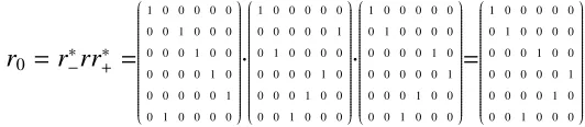
Theorem 3.21. Let r ∈ R. Then there exist unique elements r−,r0,r+ ∈ Rsuch that, (1) r =r−r0r+

(2) r0H ν∗, whereνJr andν ∈ N (3) rRr−and rLr+

(32)

Proof. We begin by showing existence. Take an arbitraryr ∈ R. By Proposition 3.9 we can find elementss∈ J Gandt∈ GJ so thatrRsandrLt. That means that we can findu,w∈W

so that su= r= wt. Now, by Proposition 3.18 we can writes =v f, forv∈W and f ∈Λ−and

t= ed, ford ∈W ande∈Λ. Considerz:= v−1_rd−1 = _{f ud}−1 =_v−1_we_.

Letν ∈ N be the unique element from that set so thatνJr. Thenν= eσ = σf, for some

σ∈W. It follows thatν∗= fσ−1 =σ−1e. It is then clear thatν∗RfRzLeLν∗, so thenzH ν∗.

Definer0 = z. Letr− = s andr+ = t. One can see from our above work that r−,r0,r+satisfy

properties (2), (3) and (4). Now we just note,

r = su=v f u= v f f ud−1d =r−f ud−1d =r−v−1wed= r−v−1weed= r−r0r+,

and so (1) is also satisfied.

For the uniqueness, suppose that we had two decompositions, r = r−r0r+ = r−0r 0

0r

0 +. It is

clear that by property (3),r−RrRr0−andr+LrLr 0

+. But since (4) tells us thatr−,r0−∈ J Gand r₊,r0₊∈ GJ, it follows by Proposition 3.9 thatr−= r0−andr+= r

0 +.

So, r = r−r0r+ = r−r0₀r+. We can write r− = σ−e−, r0 = e−σ0 = e−σ0e+ = σ0e+ and

r₊ = e₊σ₊for idempotents,e₊ ∈Λ,e− ∈ Λ−and elementsσ−, σ0, σ+ ∈W. Thus,r∗− = e−σ−−1

andr₊∗ =σ−₊1e₊. It follows that,

r−∗rr ∗

+= e−σ−−1σ−e−e−σ0e+e+σ+σ−₊1e+ =e−σ0e+= r0.

But also, sincer₀0H ν∗, we can also find aτ∈W so thatr0₀ = e−τ=e−τe+ =τe+. Then we

see thatr−∗rr ∗

+ = e−σ−−1σ−e−e−τe+e+σ+σ₊−1e+ = e−τe+ = r₀0. We conclude thatr0 = r−∗rr ∗ + = r00,

and so the decompositions are identical.

The first use of our trichotomy is that it allows us to compute the length ofrin terms ofr−,

r0andr+. This is what we will establish soon, but first we need a few minor results.

Lemma 3.22. For r ∈ R, suppose that we can write r = f u = ve for some u,v ∈W and some e, f ∈E(R). Then, Br∩rB= f Br∩rBe.

Proof. A proof is given by Renner, as Proposition 1.6 in [28].

(33)

Proof. Writer0 = f−w = we+for somew ∈ W and idempotents f−,e+. Then, by Proposition

A.1 we can write,r−= fσ= σf−andr+= τe= e+τfor someσ, τ∈W ande, f ∈E(R). Then

sincerLr₊andrRr−we can writer= f u=vefor someu,v∈W. So by Lemma 3.22, Br∩rB= f Br∩rBe= f Br−r0r+∩r−r0r+Be

⊆ r−Br0r+∩r−r0Br+ by Proposition 3.17, sincer−,r+∈ O

= σf−Br0e+τ∩σf−r0Be+τ

= σ(f−Br0e+∩ f−r0Be+)τ

= σ(f−Br0∩r0Be+)τ

= σ(Br0∩r0B)τ by Lemma 3.22, applied tor0.

We are now in position to demonstrate the length of an element in terms of our new

tri-chotomy.

Proposition 3.24. Let r ∈ R, then`(r)= `(r−)−`(e−)+`(r0)−`(e+)+`(r+), where rJe+∈Λ, rJe−∈Λ−.

Proof. Due to this result’s similarity with Theorem 3.4 in [28], the following proof is

under-standably similar.

`(r)= dim(BrB)−dim(BνB)=dim(Br)+dim(rB)−dim(Br∩rB)−dim(BνB)

Since r−Rr, we can find σ− ∈ W so thatr = r−σ−. Likewise, we can find σ+ ∈ W so that r= σ₊r₊. Now, because dimension is preserved by automorphism,

= dim(Br−)+dim(r+B)−dim(Br0∩r0B)−dim(BνB)

On the other hand,

`(r−)= dim(Br−B)−dim(BνB)=dim(Br−)−dim(BνB)

`(e−)= dim(Be−B)−dim(BνB)=dim(Be−)−dim(BνB)

`(e₊)= dim(Be₊B)−dim(BνB)=dim(e₊B)−dim(BνB)

`(r₊)= dim(Br₊B)−dim(BνB)=dim(r₊B)−dim(BνB)

by Proposition 3.8. Sincer0H ν∗we can find elements,τ−, τ+∈W, such thate−τ−=r0 =τ+e+.

Thus,

`(e−)= dim(Br0)−dim(BνB) `(e₊)= dim(r0B)−dim(BνB)

(34)

`(r−)−`(e−)+`(r0)−`(e+)+`(r+)=(dim(Br−)−dim(BνB))−(dim(Br0)−dim(BνB))

+(dim(Br0)+dim(r0B)−dim(Br0∩r0B)−dim(BνB))

−(dim(r0B)−dim(BνB))+(dim(r+B)−dim(BνB))

=dim(Br−)+dim(r+B)−dim(Br0∩r0B)−dim(BνB)

as desired.

There is a nice characterisation of the elements ofOwhen we look at the trichotomy of a given element.

Proposition 3.25. For r ∈ R, r∈ Oif and only if r0∈ N∗.

Proof. Suppose thatr0 = ν∗. It is clear thatν ∈ O, so by Proposition 3.13 thenν∗∈ O. SinceO

is a monoid, thenr = r−ν∗r+ ∈ O. On the reverse side, suppose r ∈ O. Thenr0 = r∗−rr ∗ + ∈ O.

Butr0H ν∗. Thus by Theorem 3.11,r0 =ν∗.

Now that we have a condition forOin terms of our decomposition, we can get conditions for our setsJ GandGJ.

Corollary 3.26.

(1) For r ∈ R, r ∈ J Gif and only if r0∈ N∗and r+ ∈ N. Indeed, for r∈ J G, r=rν∗ν_{is our trichotomy.}

(2) For r ∈ R, r ∈ GJ if and only if r0∈ N∗and r− ∈ N. Indeed, for r∈ GJ, r=νν∗_{r is our trichotomy.}

Proof. (1) Suppose thatr ∈ J G, then sinceJ G ⊆ O, we see thatr0 ∈ N∗. By checking our

trichotomy, we see that r− ∈ J G, and rRr−, so it follows that r = r−. We also know that r₊ ∈ GJ andr₊Lr. Let ν ∈ N be the unique element so thatrJν. Since r0Jr, it follows

thatr0 =ν∗.

We can find e ∈ Λ, f ∈ Λ− _andσ, τ _∈

W so that r = r− = τf, ν∗ = fσ−1 = σ−1e and

ν = eσ = σf. Observe that rν∗ν = (τf)(fσ−1)(σf) = τf f f = τf = r. By uniqueness of

trichotomy, this means thatr=rν∗ν, and thus,r₊∈ N.

Suppose that r0 ∈ N∗ andr+ ∈ N. Since r0JrJr+, it is clear that r0 = ν∗and r+ = ν,

(35)

r−= τf,ν∗= fσ−1= σ−1e. Then,r =r−r0r+ =(τf)(fσ−1)(σf)=τf f f =τf =r =r−. Thus,

r∈ J G.

(2) is done similarly.

Remark 3.27. It is clear to see that for ν ∈ N, that we have the trichotomy decomposition, ν= νν∗ν_{. That is, r} _{∈ N} _{if and only if r}

0∈ N∗and r−,r+ ∈ N.

While we are on the subject ofJ GandGJ, we can also obtain the following two corollar-ies.

Corollary 3.28. For r ∈ O, we can find s∈ J G∗and t∈ GJ∗so that r= r−s=tr+

Proof. By Proposition 3.25 we can writer= r−ν∗r+, wherer+B⊆ Br+. Lets= ν∗r+. We need

to show that s∗B ⊆ Bs∗. s∗ = r₊∗ν. Letν = eσand r∗₊ = τe for idempotent e, andσ, τ ∈ W. Thenr₊∗νB= r∗₊Bν =r∗₊Beν⊆ Br∗₊νby Proposition 3.17. Thuss∈ J G∗.

A similar proof gives theGJ∗result.

Corollary 3.29.

(1)Ois the smallest inverse monoid containingGJ

(2)Ois the smallest inverse monoid containingJ G

Proof. We will just prove (1), as (2) is done similarly. We know from Proposition 3.15 that

GJ ⊆ O. We know that O∗ ₌ _O

, from Proposition 3.13, and Ois a monoid, by Proposition 3.20. Thus O is an inverse monoid containing GJ. Suppose that M is an inverse monoid containingGJ. ThenGJ∗ ⊆ M∗ ₌ _M

. Take any r ∈ O. By Corollary 3.28 forr ∈ O we can finds ∈ GJ∗so thatr = sr₊. But by definition,r₊ ∈ GJ, so it follows thatr ∈ M. Thus O ⊆ M, and we conclude thatOis the smallest inverse monoid containingGJ.

The following theorem is the culmination of our trichotomy, as it allows us to describe

the Adherence order of the Renner monoid in terms of our trichotomy, when we restrict to

particular classes.

8-19-2015 12:00 AM A Study Of Green’s Relations On Algebraic Semigroups

Scholarship@Western

Scholarship@Western

A Study Of Green’s Relations On Algebraic Semigroups

A Study Of Green’s Relations On Algebraic Semigroups

(Thesis format: Monograph)

by

Allen O’Hara

Graduate Program in Mathematics

A thesis submitted in partial fulfillment

of the requirements for the degree of

Doctor of Philosophy

The School of Graduate and Postdoctoral Studies

The University of Western Ontario

London, Ontario, Canada

c

Acknowledgements

Contents

List of Appendices

1

Introduction

2

Background

2.1

Green’s Relations

2.2

Normality and Regularity

2.3

Reductive Monoids

2.4

Example

3

A New Trichotomy

3.1

Previous Results

3.2

The Trichotomy